An empirical analysis of the relationships between crude oil, gold and stock markets
Abstract
This paper analyzes the direction of the causality between crude oil, gold and stock markets for the largest economy in the world with respect to such markets, the US. To do so, we apply non-linear Granger causality tests. We find a nonlinear causal relationship among the three markets considered, with the causality going in all directions, when the full sample and different subsamples are considered. However, we find a unidirectional nonlinear causal relationship between the crude oil and gold market (with the causality only going from oil price changes to gold price changes) when the subsample runs from the first date of any year between the mid-1990s and 2001 to last available data (February 5, 2015). The latter result may explain the lack of consensus existing in the literature about the direction of the causal link between the crude oil and gold markets.
keywords:
Nonlinear Granger-causality test , Oil price , Gold price , Stock markets1 Introduction
The crude oil and gold markets are the main representative of the large commodity markets and seem to drive the price of other commodities (see Sari et al., 2010). On the one hand, gold is the leader in the precious metal markets and is considered as an investment asset. Gold is a safe haven to avoid an increase in financial risk (see Aggarwal and Lucey, 2007), a store of value (see Baur and Lucey, 2010) and a hedge against inflation (see Jaffe, 1989); consequently it is used as a fundamental investment strategy (see Baur and McDermott, 2010). On the other hand, crude oil is the main source of energy and is also used as an investment asset. Therefore, investors often include one of the two commodities –gold and crude oil– or both in their investment portfolios as a diversification strategy (see Soytas et al., 2009).
There seems to be a close relationship between the price movements of the two commodity markets, but there is no consensus on the direction of the influence. Baffes (2007), Zhang and Wei (2010) and Sari et al. (2010) found that gold prices respond significantly to changes in oil prices. However, there are some authors such as Narayan et al. (2010) and Wang and Chueh (2013) that argue that oil and gold prices affect each other.444 Bampinas and Panagiotidis (2015) found a unidirectional causality from oil prices to gold prices before the 2007/2008 crisis and a biderectional causality after the crisis. Reboredo (2013) pointed out the four mechanisms through which crude oil and gold (seen as an investment asset) are linked: a) the increase in oil prices leads to inflationary pressures (see, e.g. Hooker, 2002; Chen, 2009; Álvarez et al., 2011) that induces gold prices to increase since gold is seen as a hedge against inflation; b) high oil prices have a negative impact on economic growth (see Hamilton, 2003; Jiménez-Rodríguez and Sánchez, 2005; Kilian, 2008; Cavalcanti and Jalles, 2013) and asset values (see Reboredo, 2010), which gives rise to an increase in gold price since it is seen as an alternative asset to store value; c) higher oil prices have a positive effect on revenues in net oil exporting countries, which increases their investment in gold to maintain its share in the diversified portfolios and, consequently, gold price increases due to higher gold demand (see Melvin and Sultan, 1990); and d) when the US dollar depreciates oil prices rise (see Reboredo, 2012) and investors may use gold as a safe haven.
Given that oil and gold are used as investment asset,555As was pointed out, gold and oil are often used as a safe haven against the more traditional asset classes such as equities and bonds. they are closely related to the evolution of stock market indices since any influence on decisions about investment portfolios affects the stock market returns (see Ciner et al., 2013).
The relationship between changes in oil prices and stock market indices has been widely studied. Authors such as Jones and Kaul (1996), Sadorsky (1999), Ciner (2001), Park and Ratti (2008), Kilian and Park (2009), Ciner (2013) and Jiménez-Rodríguez (2015) found that an oil price increase has a negative impact on stock returns in oil importing countries,666 It is worth noting that there are some authors that did not find any significant impact of oil price changes on stock markets (see Huang et al., 1996; Apergis and Miller, 2009). while Bjørnland (2009) and Wang et al. (2013) found a positive impact of oil price increases on the stock market in oil exporting countries. However, there are fewer authors who have analyzed how gold prices affect stock market indices, and vice versa. Smith (2001)777Authors such as Sherman (1982), Herbst (1983) and Jaffe (1989) had previously studied the role of gold in investment portfolio.,888There are authors who state the relative benefits of including gold in the investment portfolios (see Sherman, 1982; Hillier et al., 2006; Baur and Lucey, 2010). Sherman (1982) indicated that gold has less volatility than stocks and bonds and improves overall portfolio performance. Hillier et al. (2006) found that portfolios that include precious metals outperform those with standard equity portfolios. Baur and Lucey (2010) showed that gold can be considered as a hedge against stocks on average and a safe haven in extreme stock market conditions. studied the relationship between gold prices and the US stock price indices over the 1991-2001 period. He considered four gold prices (three set in London: 10.30 a.m. fixing, 3 p.m. fixing, and closing time; and one set in New York: Handy & Harmon) and six stock price indices (the Dow Jones Industrial Average, NASDAQ, the New York Stock Exchange, Standard and Poor’s 500, Russell 3000, and Wilshire 5000) and showed evidence of a short-run relationship, but not a long-run link. He also found evidence of feedback between gold price set in the afternoon fixing and US stock price indices by using linear Granger causality test, but unidirectional causality from US stock price indices to gold price set in the morning fixing and closing time. Bhunia and Das (2012) analyzed the causal link between gold prices and Indian stock market returns, showing the bidirectional Granger-causality.
The study of the link between the two commodity markets (crude oil and gold) and the stock market indices is of interest to policymakers since the movements in the stock market has an important influence on macroeconomic variables development. To the best of our knowledge, there is no study in the related literature that analyzes the relationships between crude oil, gold and stock markets for the largest economy in the world, the US.999See the last Gross Domestic Product ranking table based on Purchasing Power Parity provided by the World Bank for 2013 (http://data.worldbank.org/data-catalog/GDP-ranking-table).
The contribution of this paper is to extend the literature on the relationships between the crude oil and gold markets and the Standards and Poor’s 500 index by analyzing the direction of the causality and by considering data from the Great Moderation onwards. To do so, we apply the nonlinear Granger causality test for the full sample and for different subsamples in order to analyze the sensitivity of the results to the use of different sample periods. Additionally, we perform the nonlinear Granger causality test for windows of one natural year from 1986 up to 2014 to investigate the causal link within each specific year.
2 Data and methodology
The empirical sample used for the present study consists of Standard and Poor’s 500 daily adjusted closing price (SP500), West Texas Intermediate crude oil spot price (WTI) and Gold Bullion LBM US/Troy Ounce (Gold) from January 2nd, 1986 to February 5th, 2015, with a total of 7351 observations. All data are available from Bloomberg. These dates were chosen in order to capture different economic moments in the relationships between the series.
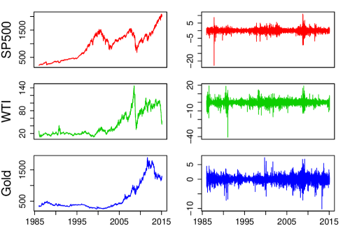
Prices were transformed into series of continuously compounded percentage returns by taking the first differences of the natural logarithm of the prices, i.e. , where is the price on day . We denote the return time series for SP500, WTI and Gold by SP500R, WTIR and GoldR, respectively. Figure 1 shows the behavior of the prices and returns for each series.
Table 1 presents the descriptive statistics of the return time series. The statistics are consistent, as expected, with some of the stylized facts of financial and economic time series (see Cont, 2001). In particular, the kurtosis indicates that return distributions are leptokurtic. Moreover, the Jarque and Bera (1987) statistic confirms returns are not normally distributed.
| Statistic | SP500R | WTIR | GoldR |
|---|---|---|---|
| Mean | |||
| Min | |||
| Max | |||
| Sd | |||
| Skewness | |||
| Kurtosis | |||
| Jarque-Bera |
We first analyze the stationarity of the variables considered101010It is worth noting that the causality tests are only valid if the variables have the same order of integration (see, e.g. Papapetrou, 2001) by applying the Augmented Dickey and Fuller (1981) test and the Residual Augmented Least Squares (RALS) test proposed by Im et al. (2014), which does not require either knowledge of a specific density function of the error term or knowledge of functional forms.
In addition to stationarity, it is standard to test for linearity of the asset variables. Thus, we apply the BDS test (Brock et al., 1996) and the Tsay (1986) test to our variables. Whereas the Tsay test is a direct test for non-linearity of a specific time series, the BDS test is an indirect test.
The aim of the Tsay (1986) test is to detect quadratic serial dependence in the data (see Tsay, 1986, for further details). The BDS test was originally developed to test for the null hypothesis of independent and identical distribution (iid) in order to detect non-random chaotic dynamics, but when it is applied to the residuals from a fitted univariate linear time series model the test uncovers any remaining dependence and the presence of an omitted nonlinear structure. Consequently, if the null hypothesis cannot be rejected, then the fitted univariate linear model cannot be rejected. However, if the null hypothesis is rejected, the fitted univariate linear model is misspecified, and in this sense, it can also be treated as a test for nonlinearity (see Zivot and Wang, 2006). There are two main advantages of choosing the BDS test: it has been shown to have more power than other linear and nonlinear tests (see Brock et al., 1991; Barnett et al., 1997); and it is nuisance-parameter-free and does not require any adjustment when applied to fitted model residuals (see F de Lima, 1996). See Brock et al. (1996) for further details.
We analyze the Granger causality relationship among the variables considered. Notice that for a strictly stationary bivariate process the process is Granger caused by if the past and current values of contain additional information of future values of that is not contained in past and current values of alone.111111See Granger (2001), Diks and Panchenko (2006) and Wolski (2014) for a formal definition of Granger causality. Recently, there has been an increase of interest in nonparametric versions of the Granger non-causality hypothesis against linear and nonlinear Granger causality (see Hiemstra and Jones, 1994; Bell et al., 1996; Su and White, 2008). Given that the linear Granger causality test might fail to uncover nonlinear causal relationships, we use the Diks and Panchenko (2006) nonlinear Granger causality test (hereafter, DP test).
The DP test is a nonparametric Granger causality test based on the use of the correlation integral between time series and based on Baek and Brock (1992) but without the assumption of the time series being mutually and individually independent and identically distributed. It has has also been shown to be more display short-term temporal dependence, since it reduces the over-rejection whenever the null hypothesis is true.
We next describe the DP test closely following the description offered by Diks and Panchenko (2006). It is denoted by and the delay vector of and , respectively. The null hypothesis tested is the lack of causality, that is, that past observations of do not contain additional information about :
| (1) |
Considering a strictly stationary bivariate time series , the null hypothesis is a statement about the invariant distribution of the dimensional vector , with . Assuming that the null hypothesis is a statement about the invariant distribution of , the time subscript can be dropped and it can be just written as . To simplify the test description, it is assumed that . Thus, the conditional distribution of given is the same, under the null hypothesis, as that of given . In terms of joint probability density function, , and its marginals, the null hypothesis has to ensure:
| (2) |
for each vector in the support of . Thus, it can be stated that and are independent conditionally on for each value of (see Bekiros and Diks, 2008; Wolski, 2014). Diks and Panchenko (2006) show that the reformulated null hypothesis implies the statistic to be noted as
| (3) |
where the proposed estimator for is:
| (4) |
where , with · being an indicator function, being the maximum norm and being the bandwidth which depends on the sample size. Denoting as the local density estimator of the vector at ,i.e.,
| (5) |
the test statistic simplifies to
| (6) |
Considering one lag (which implies that ), for a sequence with bandwidth , where and , the test statistic satisfies
| (7) |
where is an estimator of the asymptotic standard error of · and denotes convergence in distribution. We implement a one-tailed version of the test, rejecting the null hypothesis if the left hand side of the equation is too large. See Diks and Panchenko (2006) for further details.
3 Empirical Results
| Series | SP500 | WTI | Gold |
|---|---|---|---|
| Series in levels | |||
| With trend and intercept | |||
| ADF | |||
| RALS | |||
| With drift | |||
| ADF | |||
| RALS | |||
| Series in first differences | SP500R | WTIR | GoldR |
| With trend and intercept | |||
| ADF | |||
| RALS | |||
| With drift | |||
| ADF | |||
| RALS |
-
1.
Notes: The null hypothesis is that there is a unit root. The lag was selected by using Bayesian Information Criteria. One/two/three asterisks mean a -value less than 10%, 5% and 1%, respectively.
Table 2 shows the results of the ADF and the RALS. Both tests fail to reject the null hypothesis that the series in levels are non-stationary and reject the null hypothesis that the series in first differences are non-stationary at the 5% critical level. Thus, the series in levels are integrated of order one, .
| Series | |||||
|---|---|---|---|---|---|
| 2 | |||||
| SP500R | 3 | ||||
| 4 | |||||
| 2 | |||||
| WTIR | 3 | ||||
| 4 | |||||
| 2 | |||||
| GoldR | 3 | ||||
| 4 |
-
1.
Notes: The null hypothesis is that the residuals are iid. One/two/three asterisks mean a -value less than 10%, 5% and 1%, respectively.
We perform the BDS test on the residuals of the return time series for dimensions up to 4 and values of equal to 0.5, , 1.5, where represents the standard deviation of the return time series . The results of the tests show the rejection of the null hypothesis in all cases (see Table 3), from which the nonlinearity of the series can be inferred.
| Lag | SP500R | WTIR | GoldR |
|---|---|---|---|
| 1 | |||
| 2 | |||
| 3 | |||
| 4 | |||
| 5 | |||
| 6 | |||
| 7 |
-
1.
Note: The null is that the series are linear. One/two/three asterisks mean a -value less than 10%, 5% and 1%, respectively.
Table 4 shows the results of the Tsay (1986) test, showing that we reject the null hypothesis of linearity and confirming results found with the BDS test. Therefore, there seems to be a nonlinear univariate structure behind all our time series. This information is considered and we use the nonlinear Granger-causality test proposed by Diks and Panchenko (2006).
We apply the DP test to the delinearized series. The series have been delinearized by using a VAR filter, whose lag length is chosen on the basis of Bayesian Information Criterion. As Hiemstra and Jones (1994) and Bampinas and Panagiotidis (2015) state ”by removing linear predictive power with a VAR model, any causal linkage from one residual series of the VAR model to another can be considered as nonlinear predictive power”. We perform the DP test for the full sample and for different subsamples to investigate the sensitivity of such results to the use of different sample periods. Additionally, we apply the DP test for windows of one natural year from 1986 up to 2014 in order to analyse the causal link within each specific year.
Table 5 presents the results of DP test for the full sample (January 2, 1986 - February 5, 2015) in a compact way following the simplifying notation of Bekiros and Diks (2008), who consider one/two/three asterisks to indicate that the corresponding p-value of a test is lower than 10%, 5% and 1%, respectively. Directional causalities will be denoted by the functional representation , i.e., means that the VAR filtered series does not Granger cause the VAR filtered series. () denotes the value of for the filter of the series {}, {} and {}. Finally, represents SP500R, refers to WTIR and is GoldR.
| Lag | ||||||
|---|---|---|---|---|---|---|
| 1 | ||||||
| 2 | ||||||
| 3 | ||||||
| 4 | ||||||
| 5 |
-
1.
Note: Note: One/two/three asterisks mean a -value less than 10%, 5% and 1%, respectively. The null hypothesis is that does not Granger cause (i.e., ). Denoting SP500R, WTIR and GoldR as , and , respectively.
Table 5 indicates that the three markets considered (the crude oil, gold and stock markets) are interrelated, with the causality going in all directions. The bidirectional causality between the price movements of the two commodity markets is in concordance with Narayan et al. (2010) and Wang and Chueh (2013), showing the mutual influence of the two investment assets since the Great Moderation. Moreover, the bidirectional causality between the Standard and Poor’s 500 returns and changes in the price of the two commodities implies that movements in S&P’s 500 index may be monitored by observing changes in commodity prices and vice versa. The feedback relationship between the crude oil and stock markets is in line with Ciner (2001), among others. The bidirectional causal relationship between the gold market and the US stock price index is very relevant and has been only found by Smith (2001) for a specific gold price (3 p.m. fixing).
| Ending year | sample size | |||||||
|---|---|---|---|---|---|---|---|---|
| 1991 | 1.15 | 1517 | * | * | * | |||
| 1992 | 1.05 | 1773 | ** | * | * | * | ** | * |
| 1993 | 1.00 | 2032 | ** | * | * | * | ** | ** |
| 1994 | 0.97 | 2289 | *** | * | * | ** | ** | ** |
| 1995 | 0.96 | 2541 | *** | ** | * | * | *** | *** |
| 1996 | 0.94 | 2795 | *** | ** | ** | * | * | * |
| 1997 | 0.92 | 3048 | *** | ** | ** | ** | * | * |
| 1998 | 0.90 | 3300 | ** | * | * | * | * | ** |
| 1999 | 0.88 | 3552 | *** | * | * | ** | ** | ** |
| 2000 | 0.86 | 3804 | *** | * | ** | ** | * | ** |
| 2001 | 0.84 | 4053 | *** | * | ** | *** | * | * |
| 2002 | 0.82 | 4305 | *** | * | *** | ** | * | ** |
| 2003 | 0.80 | 4557 | *** | * | ** | *** | ** | *** |
| 2004 | 0.78 | 4809 | *** | * | ** | ** | ** | *** |
| 2005 | 0.76 | 5061 | *** | ** | ** | ** | ** | *** |
| 2006 | 0.75 | 5312 | *** | * | * | ** | ** | *** |
| 2007 | 0.74 | 5563 | *** | * | * | ** | ** | ** |
| 2008 | 0.74 | 5816 | *** | ** | ** | ** | ** | *** |
| 2009 | 0.73 | 6068 | *** | ** | *** | *** | ** | *** |
| 2010 | 0.73 | 6320 | *** | * | *** | *** | * | * |
| 2011 | 0.72 | 6572 | *** | ** | ** | ** | ** | *** |
| 2012 | 0.71 | 6822 | *** | * | *** | *** | * | *** |
| 2013 | 0.70 | 7074 | *** | ** | *** | *** | * | *** |
| 2014 | 0.69 | 7326 | *** | ** | *** | *** | * | * |
-
1.
Note: One, two and three asterisks mean a -value less than 10%, 5% and 1%, respectively. The null hypothesis is that does not Granger cause (i.e., ). Denoting SP500R, WTIR and GoldR as , and , respectively. Even though the DP test is run considering different lags (), it is only reported for each sample the lowest significance level (*,** or ***) for the cases in which causality appears at every lag considered. If no asterisk appears for a particular sample, it means that the causality may exist at some specific lag but not at all possible lags considered.
To analyze whether the results obtained depends on the sample period considered we apply the DP test to different subsamples, with subsamples containing a minimum of five years of observations. Whereas Table 6 presents the results for the subsamples that run from January 2, 1986 to the last available observation of the year indicated under the notation ”ending year”, Table 7 shows the results for the subsamples that run from the first available observation of the year indicated under the notation ”starting year” to February 5, 2015. Both Tables only report for each sample the lowest significance level (*,** or ***) for the cases in which causality appears at every lag considered. If no asterisk appears for a particular sample, it means that the causality may exist at some specific lag but not at all possible lags considered.
| Starting year | sample size | |||||||
|---|---|---|---|---|---|---|---|---|
| 1987 | 0.70 | 7099 | ** | * | *** | *** | ** | * |
| 1988 | 0.71 | 6846 | *** | ** | *** | *** | * | *** |
| 1989 | 0.72 | 6592 | *** | ** | *** | *** | * | ** |
| 1990 | 0.72 | 6340 | *** | ** | *** | *** | * | ** |
| 1991 | 0.73 | 6086 | *** | * | *** | *** | * | * |
| 1992 | 0.74 | 5833 | *** | * | *** | *** | ** | * |
| 1993 | 0.74 | 5577 | *** | ** | *** | *** | *** | * |
| 1994 | 0.75 | 5318 | ** | * | *** | *** | * | * |
| 1995 | 0.76 | 5061 | ** | * | *** | *** | *** | * |
| 1996 | 0.77 | 4809 | ** | ** | *** | ** | * | |
| 1997 | 0.79 | 4555 | *** | *** | *** | ** | ||
| 1998 | 0.82 | 4302 | *** | ** | *** | *** | ||
| 1999 | 0.84 | 4050 | *** | ** | *** | *** | ** | |
| 2000 | 0.86 | 3798 | ** | ** | *** | *** | ** | |
| 2001 | 0.88 | 3546 | *** | * | *** | *** | ** | |
| 2002 | 0.90 | 3297 | ** | ** | *** | ** | *** | * |
| 2003 | 0.85 | 3045 | ** | ** | ** | ** | * | * |
| 2004 | 0.97 | 2793 | * | * | *** | ** | * | * |
| 2005 | 1.00 | 2541 | ** | ** | *** | ** | ** | * |
| 2006 | 0.98 | 2289 | ** | * | *** | *** | * | ** |
| 2007 | 1.00 | 2038 | *** | ** | *** | *** | * | * |
| 2008 | 1.05 | 1787 | * | ** | *** | *** | * | * |
| 2009 | 1.09 | 1534 | * | * | *** | *** | * | * |
-
1.
Note: One, two and three asterisks mean a -value less than 10%, 5% and 1%, respectively. The null hypothesis is that does not Granger cause (i.e., ). Denoting SP500R, WTIR and GoldR as , and , respectively. Even though the DP test is run considering different lags (), it is only reported for each sample the lowest significance level (*,** or ***) for the cases in which causality appears at every lag considered. If no asterisk appears for a particular sample, it means that the causality may exist at some specific lag but not at all possible lags considered.
Tables 6 and 7 show that we reject the null hypothesis of that S&P’s 500 returns do not Granger cause oil price changes at the 1% critical level for most subsamples. We also reject that oil price changes do not Granger cause S&P’s 500 returns at a 5% critical level for an important number of subsamples. Thus, the bidirectional causality between the crude oil and stock markets found for the full sample is verified when different subsamples are considered, although the causality from oil price changes to S&P’s 500 returns seems to weaken depending on when the sample starts and ends.
| years | ||||||
|---|---|---|---|---|---|---|
| 1986 | ||||||
| 1987 | * | |||||
| 1989 | * | * | ||||
| 1990 | * | ** | ** | * | ||
| 1991 | ** | * | ** | ** | ||
| 1992 | * | * | ||||
| 1993 | ||||||
| 1994 | * | * | * | |||
| 1995 | * | |||||
| 1996 | * | |||||
| 1997 | * | * | ||||
| 1998 | ||||||
| 1999 | * | |||||
| 2000 | * | |||||
| 2001 | ||||||
| 2002 | * | |||||
| 2003 | * | * | * | |||
| 2004 | * | * | ** | |||
| 2005 | * | * | ||||
| 2006 | * | * | ||||
| 2007 | * | * | * | |||
| 2008 | *** | ** | ** | * | ** | * |
| 2009 | ** | * | * | * | * | ** |
| 2010 | * | * | * | |||
| 2011 | * | ** | * | |||
| 2012 | * | |||||
| 2013 | * | * | * | * | ||
| 2014 | ** | ** | * |
-
1.
Note: One, two and three asterisks mean a -value less than 10%, 5% and 1%, respectively. The null hypothesis is that does not Granger cause (i.e., ). Denoting SP500R, WTIR and GoldR as , and , respectively. Even though the DP test is run considering different lags (), it is only reported for each sample the lowest significance level (*,** or ***) for the cases in which causality appears at every lag considered. If no asterisk appears for a particular sample, it means that the causality may exist at some specific lag but not at all possible lags considered.
Tables 6 and 7 also indicate the rejection of the null hypothesis when the returns of the gold and stock markets are considered, showing so a bidirectional causality for almost all subsamples and confirming the results obtained for the full sample. Additionally, these tables reveal the feedback relationship between the crude oil and gold markets when the sample starts in January 2, 1986 and ends in the last available observation of any year beyon 1991. However, a unilateral Granger causality was found from oil price changes to gold price changes when the sample starts in the first available observation of any year between the mid-1990s and 2001 and ends in February 5, 2015. This may explain why some authors (see, e.g. Zhang and Wei, 2010) find a unilateral causality.
Finally, Table 8 reports the results of the DP test for windows of one natural year from 1986 up to 2014, although these results have to be considered with caution since the DP test is an asymptotic test. Table 8 shows no evidence of a causality within most of the years considered. The main exception to this is for the years 2008 and 2009 (the period of global financial crisis), where the three markets appear interrelated. These causal relationships might be due to the fact that gold is considered a safe haven for investors in times of financial crisis and economic instability and also due to investors seeking refuge on gold and other commodities such as oil and energy derivatives after the collapse of the real state market.
4 Conclusions
This paper provides new evidence on a nonlinear causal link among the three markets considered (with the causality going in all directions) for the full sample, for subsamples starting in January 2, 1986 and ending in the last available observation of any year beyond 1991 and for subsamples starting in the first available observation of any year beyond 1987 and ending in February 5, 2015. The only exception to this is the existence of a nonlinear unidirectional causal relationship between the crude oil and gold market (with the causality only going from oil price changes to gold price changes) for subsamples that going from the first date of any year between the mid-1990s and 2001 to February 5, 2015. Therefore, the causality between the price movements of the crude oil and gold markets seems highly dependent on the sample used, which may explain the contradictory results found in the related literature.
The causal link found among the three markets implies that changes in the S&P’s 500 index may be monitored by observing changes in the returns of the two commodity markets considered (and vice versa), which is valuable for policymakers
Acknowledgments
Rebeca Jiménez-Rodríguez acknowledges support from the Ministerio de Economía y Competitividad under Research Grant ECO2012-38860-C02-01.
References
References
- Aggarwal and Lucey (2007) Aggarwal, R., Lucey, B. M., 2007. Psychological barriers in gold prices? Review of Financial Economics 16 (2), 217–230.
- Álvarez et al. (2011) Álvarez, L. J., Hurtado, S., Sánchez, I., Thomas, C., 2011. The impact of oil price changes on Spanish and euro area consumer price inflation. Economic Modelling 28 (1), 422–431.
- Apergis and Miller (2009) Apergis, N., Miller, S. M., 2009. Do structural oil-market shocks affect stock prices? Energy Economics 31 (4), 569–575.
- Baek and Brock (1992) Baek, E., Brock, W., 1992. A general test for nonlinear granger causality: Bivariate model. Iowa State University and University of Wisconsin at Madison Working Paper.
- Baffes (2007) Baffes, J., 2007. Oil spills on other commodities. Resources Policy 32 (3), 126–134.
- Bampinas and Panagiotidis (2015) Bampinas, G., Panagiotidis, T., 2015. On the relationship between oil and gold before and after financial crisis: linear, nonlinear and time-varying causality testing, forthcoming in Studies in Nonlinear Dynamics & Econometrics.
- Barnett et al. (1997) Barnett, W. A., Gallant, A. R., Hinich, M. J., Jungeilges, J. A., Kaplan, D. T., Jensen, M. J., 1997. A single-blind controlled competition among tests for nonlinearity and chaos. Journal of Econometrics 82 (1), 157–192.
- Baur and Lucey (2010) Baur, D. G., Lucey, B. M., 2010. Is gold a hedge or a safe haven? An analysis of stocks, bonds and gold. Financial Review 45 (2), 217–229.
- Baur and McDermott (2010) Baur, D. G., McDermott, T. K., 2010. Is gold a safe haven? International evidence. Journal of Banking & Finance 34 (8), 1886–1898.
- Bekiros and Diks (2008) Bekiros, S. D., Diks, C. G., 2008. The relationship between crude oil spot and futures prices: Cointegration, linear and nonlinear causality. Energy Economics 30 (5), 2673–2685.
- Bell et al. (1996) Bell, D., Kay, J., Malley, J., 1996. A non-parametric approach to non-linear causality testing. Economics Letters 51 (1), 7–18.
- Bhunia and Das (2012) Bhunia, A., Das, A., 2012. Association between gold prices and stock market returns: Empirical evidence from NSE. Journal of Exclusive Management Science 1 (2), 1–7.
- Bjørnland (2009) Bjørnland, H. C., 2009. Oil price shocks and stock market booms in an oil exporting country. Scottish Journal of Political Economy 56 (2), 232–254.
- Brock et al. (1996) Brock, W., Scheinkman, J. A., Dechert, W. D., LeBaron, B., 1996. A test for independence based on the correlation dimension. Econometric Reviews 15 (3), 197–235.
- Brock et al. (1991) Brock, W. A., Hsieh, D. A., LeBaron, B. D., 1991. Nonlinear Dynamics, Chaos, and Instability: Statistical Theory and Economic Evidence. MIT press.
- Cavalcanti and Jalles (2013) Cavalcanti, T., Jalles, J. T., 2013. Macroeconomic effects of oil price shocks in Brazil and in the United States. Applied Energy 104, 475–486.
- Chen (2009) Chen, S.-S., 2009. Revisiting the inflationary effects of oil prices. The Energy Journal 30 (4), 141–154.
- Ciner (2001) Ciner, C., 2001. Energy shocks and financial markets: nonlinear linkages. Studies in Nonlinear Dynamics & Econometrics 5 (3), 203–212.
- Ciner (2013) Ciner, C., 2013. Oil and stock returns: Frequency domain evidence. Journal of International Financial Markets, Institutions and Money 23, 1–11.
- Ciner et al. (2013) Ciner, C., Gurdgiev, C., Lucey, B. M., 2013. Hedges and safe havens: An examination of stocks, bonds, gold, oil and exchange rates. International Review of Financial Analysis 29, 202–211.
- Cont (2001) Cont, R., 2001. Empirical properties of asset returns: stylized facts and statistical issues. Quantitative Finance 1, 223–236.
- Dickey and Fuller (1981) Dickey, D. A., Fuller, W. A., 1981. Likelihood ratio statistics for autoregressive time series with a unit root. Econometrica: Journal of the Econometric Society, 1057–1072.
- Diks and Panchenko (2006) Diks, C., Panchenko, V., 2006. A new statistic and practical guidelines for nonparametric granger causality testing. Journal of Economic Dynamics and Control 30 (9), 1647–1669.
- F de Lima (1996) F de Lima, P. J., 1996. Nuisance parameter free properties of correlation integral based statistics. Econometric Reviews 15 (3), 237–259.
- Granger (2001) Granger, C. W., 2001. Essays in Econometrics; Collected Papers of Clive W. J. Granger. Vol. 32. Cambridge University Press, Ch. Forecasting white noise, pp. 457–471.
- Hamilton (2003) Hamilton, J. D., 2003. What is an oil shock? Journal of Econometrics 113 (2), 363–398.
- Herbst (1983) Herbst, A. F., 1983. Gold versus US common stocks: Some evidence on inflation hedge performance and cyclical behavior. Financial Analysts Journal 39 (1), 66–74.
- Hiemstra and Jones (1994) Hiemstra, C., Jones, J. D., 1994. Testing for linear and nonlinear granger causality in the stock price-volume relation. The Journal of Finance 49 (5), 1639–1664.
- Hillier et al. (2006) Hillier, D., Draper, P., Faff, R., 2006. Do precious metals shine? An investment perspective. Financial Analysts Journal 62 (2), 98–106.
- Hooker (2002) Hooker, M. A., 2002. Are oil shocks inflationary?: Asymmetric and nonlinear specifications versus changes in regime. Journal of Money, Credit, and Banking 34 (2), 540–561.
- Huang et al. (1996) Huang, R. D., Masulis, R. W., Stoll, H. R., 1996. Energy shocks and financial markets. Journal of Futures Markets 16 (1), 1–27.
- Im et al. (2014) Im, K. S., Lee, J., Tieslau, M. A., 2014. More powerful unit root tests with non-normal errors. In: Festschrift Honor Peter Schmidt. Springer, New York, pp. 315–342.
- Jaffe (1989) Jaffe, J. F., 1989. Gold and gold stocks as investments for institutional portfolios. Financial Analysts Journal 45 (2), 53–59.
- Jarque and Bera (1987) Jarque, C., Bera, A., 1987. A test for normality of observations and regression residuals. Stat. Rev. / Rev. Int. Stat. 55, 163–172.
- Jiménez-Rodríguez (2015) Jiménez-Rodríguez, R., 2015. Oil price shocks and stock markets: Testing for non-linearity. Empirical Economics 48 (3), 1079–1102.
- Jiménez-Rodríguez and Sánchez (2005) Jiménez-Rodríguez, R., Sánchez, M., 2005. Oil price shocks and real GDP growth: Empirical evidence for some OECD countries. Applied Economics 37 (2), 201–228.
- Jones and Kaul (1996) Jones, C. M., Kaul, G., 1996. Oil and the stock markets. The Journal of Finance 51 (2), 463–491.
- Kilian (2008) Kilian, L., 2008. Exogenous oil supply shocks: how big are they and how much do they matter for the us economy? The Review of Economics and Statistics 90 (2), 216–240.
- Kilian and Park (2009) Kilian, L., Park, C., 2009. The impact of oil price shocks on the us stock market. International Economic Review 50 (4), 1267–1287.
- Melvin and Sultan (1990) Melvin, M., Sultan, J., 1990. South african political unrest, oil prices, and the time varying risk premium in the gold futures market. Journal of Futures Markets 10 (2), 103–111.
- Narayan et al. (2010) Narayan, P. K., Narayan, S., Zheng, X., 2010. Gold and oil futures markets: Are markets efficient? Applied Energy 87 (10), 3299–3303.
- Papapetrou (2001) Papapetrou, E., 2001. Oil price shocks, stock market, economic activity and employment in greece. Energy Economics 23 (5), 511–532.
- Park and Ratti (2008) Park, J., Ratti, R. A., 2008. Oil price shocks and stock markets in the US and 13 European countries. Energy Economics 30 (5), 2587–2608.
- Reboredo (2010) Reboredo, J. C., 2010. Nonlinear effects of oil shocks on stock returns: A Markov-switching approach. Applied Economics 42 (29), 3735–3744.
- Reboredo (2012) Reboredo, J. C., 2012. Modelling oil price and exchange rate co-movements. Journal of Policy Modeling 34 (3), 419–440.
- Reboredo (2013) Reboredo, J. C., 2013. Is gold a hedge or safe haven against oil price movements? Resources Policy 38 (2), 130–137.
- Sadorsky (1999) Sadorsky, P., 1999. Oil price shocks and stock market activity. Energy Economics 21 (5), 449–469.
- Sari et al. (2010) Sari, R., Hammoudeh, S., Soytas, U., 2010. Dynamics of oil price, precious metal prices, and exchange rate. Energy Economics 32 (2), 351–362.
- Sherman (1982) Sherman, E. J., 1982. Gold: a conservative, prudent diversifier. The Journal of Portfolio Management 8 (3), 21–27.
- Smith (2001) Smith, G., 2001. The price of gold and stock price indices for the United States. The World Gold Council 8, 1–16.
- Soytas et al. (2009) Soytas, U., Sari, R., Hammoudeh, S., Hacihasanoglu, E., 2009. World oil prices, precious metal prices and macroeconomy in turkey. Energy Policy 37 (12), 5557–5566.
- Su and White (2008) Su, L., White, H., 2008. A nonparametric hellinger metric test for conditional independence. Econometric Theory 24 (04), 829–864.
- Tsay (1986) Tsay, R. S., 1986. Nonlinearity tests for time series. Biometrika 73 (2), 461–466.
- Wang et al. (2013) Wang, Y., Wu, C., Yang, L., 2013. Oil price shocks and stock market activities: Evidence from oil-importing and oil-exporting countries. Journal of Comparative Economics 41 (4), 1220–1239.
- Wang and Chueh (2013) Wang, Y. S., Chueh, Y. L., 2013. Dynamic transmission effects between the interest rate, the us dollar, and gold and crude oil prices. Economic Modelling 30, 792–798.
- Wolski (2014) Wolski, M., 2014. Essays in nonlinear dynamics in economics and econometrics with applications to monetary policy and banking. Phd thesis, Faculteit Economie en Bedrijfskunde, Universiteit van Amsterdam, Amsterdam.
- Zhang and Wei (2010) Zhang, Y.-J., Wei, Y.-M., 2010. The crude oil market and the gold market: Evidence for cointegration, causality and price discovery. Resources Policy 35 (3), 168–177.
- Zivot and Wang (2006) Zivot, E., Wang, J., 2006. Modeling Financial Time Series with S-PLUS. Springer.