Accurate atomic quantum defects from particle-particle random phase approximation
Abstract
The accuracy of calculations of atomic Rydberg excitations cannot be judged by the usual measures, such as mean unsigned errors of many transitions. We show how to use quantum defect theory to (a) separate errors due to approximate ionization potentials, (b) extract smooth quantum defects to compare with experiment, and (c) quantify those defects with a few characteristic parameters. The particle-particle random phase approximation (pp-RPA) produces excellent Rydberg transitions that are an order of magnitude more accurate than those of time-dependent density functional theory with standard approximations. We even extract reasonably accurate defects from the lithium Rydberg series, despite the reference being open-shell. Our methodology can be applied to any Rydberg series of excitations with 4 transitions or more to extract the underlying threshold energy and characteristic quantum defect parameters. Our pp-RPA results set a demanding challenge for other excitation methods to match.
I Introduction
An accurate description of electronic excited states has always been a major goal for theoretical and computational chemists. Nowadays, linear-response time-dependent density functional theory (LR-TDDFT) Runge_1984_997 ; Casida1996 ; Petersilka_1996_1212 ; Ullrich2012 has become the standard workhorse for practical applications, because of the favorable balance between accuracy and computational cost. However, there are a variety of well-established limitations of TDDFT with the standard semilocal functionals Burke_2005_62206 . These challenges include double excitations, charge transfer (CT) excitations, and Rydberg excitationsTozer_2000_2117 ; Cave_2004_39 ; Tozer_1999_859 ; Dreuw_2003_2943 ; Dreuw_2005_4009 ; Ullrich2012 . Although many of these problems can be ameliorated by using range-separated Leininger_1997_151 ; Iikura_2001_3540 or more accurate asymptotic-corrected response kernels Leeuwen_1994_2421 ; Tozer_1998_10180 ; Casida_2000_8918 ; Wu_2003_2978 , the results are not always satisfactory, and a more careful examination beyond the usual tabulations of mean absolute errors is required to check for an accurate Rydberg series.
Quantum defect (QD) theorySeaton_1983_167 has long been applied as a test for atomic Rydberg excitationsFaassen_2006_94102 . In the long history of quantum mechanics, the QD was originally introduced to empirically describe weak electron penetration effects relative to strong shielding effect Sommerfeld_1916_1 ; Seaton_1983_167 . Later, systematic derivations were given, creating a non-empirical theory Seaton_1983_167 . The QD can also be applied to describe many molecular Rydberg states Guerout_2004_3043 ; Guerout_2004_3057 ; Petsalakis_2003_2004 ; Merkt_1997_675 ; Herzberg_1987_27 .
In the present work, we restrict ourselves to atomic Rydberg series. QDs are often given as lists, with the index corresponding to the principal quantum number. But the crucial feature of QDs is that they are smoothly varying functions of the energy. In fact, they even merge continuously with scattering phase shifts across the ionization thresholdFB09 . We use the smoothness feature to create our procedure for extracting QDs from lists of excitation energies. In earlier work, Van Faassen and Burke Faassen_2006_94102 analyzed the singlet and triplet spin-states of the S- and P- series for atomic helium, beryllium and neon as test cases for standard TDDFT. Although excitation energy errors were no more than a few millihartree, the delicate QD results exposed their limitations. With a ground-state DFT calculation that yields a potential with the correct asymptotic decay (although see Ref. WBb05 for a way around even this restriction), QDs that were reasonably but not highly accurate were usually found with semilocal approximations to the kernel in TDDFT. Later, the D series in Be was shown to be very poorly described by TDDFTFaassen_2006_410 .
Recently, two of us developed the particle-particle random phase approximation (pp-RPA) and the particle-particle Tamm-Dancoff approximation (pp-TDA) theory for calculation of challenging excitations such as double excitations, charge transfer excitations, Rydberg excitations, and excitations in diradicals. Yang_2013_224105 ; Yang_2014_124104 ; Yang_2015_4923 . Good excitation energies were typically found with a relatively low computational cost, where is the number of virtual orbitals.Yang_2014_124104 Thus pp-RPA and pp-TDA are promising methods that complement standard LR-TDDFT, especially for these challenging cases. In the present work, we develop QD analysis to more stringently test these methods, and compare them to TDDFT.
| Transition | Expt. | pp-TDA | ALDA |
|---|---|---|---|
| 2s2p | 0.1940 | 0.1959 | 0.1868 |
| 2s3p | 0.2742 | 0.2737 | 0.2710 |
| 2s4p | 0.3054 | 0.3047 | 0.3048 |
| 2s5p | 0.3195 | 0.3186 | 0.3194 |
| MSE (mH) | -0.1 | -2.8 | |
| MUE (mH) | 1.1 | 2.8 | |
| 2s6p | 0.3269 | 0.3259 | 0.3269 |
| 2s7p | 0.3313 | 0.3302 | 0.3313 |
| 2s8p | 0.3340 | 0.3329 | 0.3341 |
| 2s9p | 0.3359 | 0.3348 | 0.3359 |
| 2s10p | 0.3372 | 0.3361 | 0.3372 |
| 2s11p | 0.3382 | 0.3370 | 0.3382 |
| 2s12p | 0.3389 | 0.3378 | 0.3389 |
| MSE (mH) | -1.1 | 0.0 | |
| MUE (mH) | 1.1 | 0.0 | |
| All | |||
| MSE (mH) | -0.7 | -1.0 | |
| MUE (mH) | 1.1 | 1.0 |
To illustrate the need for the QD analysis, we first analyze a Rydberg series using the traditional methods of measuring errors in electronic structure methods. In Table 1, we list the lowest 11 excitation energies in the Be P singlet series. We include the experimental values, the pp-TDA results (details given later) and TDDFT calculations using the ALDA kernel and exact ground-state KS potential (see Ref. Faassen_2006_94102 ). We see that, for the lowest transition frequencies, pp-TDA is far better than ALDA. But beyond about the fifth transition, the pp-TDA error stops decreasing, while the ALDA error keeps getting smaller. Thus, when we average over transitions 2-5, pp-TDA is clearly much better than ALDA. But when average over 6-12, the order has been reversed, so that ALDA now appears better when averaged over all transition. This trend would continue, with the mean errors in ALDA going to zero as the total number of transitions included increases, while that of pp-TDA tends to about 1 mH. However, we show below that this is entirely an artifact of the error in the ionization potential (IP) of pp-TDA, which is absent in the TDDFT calculations by virtue of using the exact KS potential. As the number of transitions included increases, the errors reflect simply the error in the IP. For any finite number, there is no way to separate the two effects by this means. In fact, we show below that the pp-TDA results listed here are almost an order of magnitude better than the TDDFT results.
II Theory
II.1 Quantum defect theory as a measure of Rydberg excitations
Consider a Rydberg series of excited states of a neutral atom, with energies below the ionization threshold, where runs from the first allowed excitation and is unbounded. The QD for this series is defined by:
| (1) |
i.e., as grows, approaches 0 ever more slowly, mimicking the behavior of a H-atom series, but with small deviations. The QD is a dimensionless measure of the deviation from a pure Hydrogenic series.
The key ingredient of our analysis is to generalize the QD as a function of index to a continuous function of , i.e., Faassen_2006_94102 ; Faassen_2006_410 , with the requirement that
| (2) |
In fact, all QDs are smooth functions of in practice. We make the further assumption that, on the scale of energies spanned by the series, is not strongly varying, and can usually be well-approximated by a simple parabola:
| (3) |
Thus an entire, infinite Rydberg series can be very accurately represented by three real numbers, one of which () is simply the quantum defect at threshold , and the accuracy of an approximate Rydberg series can be judged by the accuracy of its approximation for . For the rest of this paper, we approximate all such curves by parabolas.
But transition frequencies are measured or calculated relative to the ground state, so a fourth number, the IP, enters:
| (4) |
or
| (5) |
While might be known very accurately for a given experiment, in calculations its precise value is slightly affected by the limitations of a calculation, such as finite basis sets. As grows, even tiny errors in will cause to become highly inaccurate. Thus our procedure is designed to accommodate uncertainty in the value of , and below we test this in cases where is known.
Expanding in a Taylor series around , we find
| (6) |
Thus, given at least 4 transition frequencies, we can fit a Rydberg series to find the best four parameters, which gives us our best estimate for . Note that we have added a tilde to each of , because these parameters are not best estimated by this procedure, as we performed an expansion around to find Eq. (6). Thus, in a second fitting step, we fix , and refit via Eqs. (3-5), yielding our best estimate for these. Once we have values for , we plot the QD as a function of and see how well a method performs.
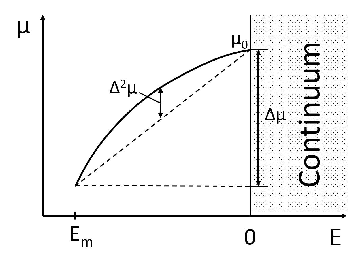
A final piece of methodology is to convert the parameters to others that are easier to interpret. Denote by the minimum value of , i.e, the lowest transition in the series. We then write
| (7) |
The parameters have been carefully chosen to have an immediate physical interpretation. Here is the QD at threshold, while , the QD shift, is the change in QD from the lowest transition to the threshold. A negative value means the QD drops, a positive value means it is rising, and is the fit value of . Lastly, we call the QD curvature, and is the maximum deviation from linearity, which occurs at . A negative value means the curve is convex, a positive value means concave. This simple geometric interpretation is shown in Fig 1. We will use these values to judge and interpret the accuracy of approximate calculations of Rydberg series.
II.2 Basic theory on pp-RPA
The pp-RPA can be derived in a variety of independent ways, including via the adiabatic connection-pairing matrix fluctuationsAggelen_2013_30501 ; Aggelen_2014_18A511 , equations of motion Rowe_1968_153 ; Ring2004 ; Yang_2013_174110 , and time-dependent density functional theory with a pairing field Peng_2014_18A522 . The key working equation of pp-RPA is a generalized eigenvalue equation
| (8) |
with
| (9) | ||||
where are virtual orbital indices and are occupied orbital indices with the restrictions that , , and . The brackets are defined as
| (10) |
and . This equation describes the transition process of adding or removing two electrons from a system. In an excitation energy calculation, we usually adopt a two-electron deficient reference and investigate its two-electron addition processes, yielding a series of neutral states including both the ground and electronically excited states. Differences between transition energies are neutral excitation energies with
| (11) |
where and denote the number of electrons, and and denote the ground and excited states, respectively. By solving Eq. (8) and processing the output with Eq. (11), we obtain the excitation energies for the -electron system.
There is a corresponding Tamm-Dancoff approximation (pp-TDA) to pp-RPA. We simply set . The result of pp-TDA is often similar to pp-RPA, and the difference is negligible in small systems with limited number of electrons. Therefore, we use the pp-TDA throughout this paper, which is slightly cheaper than pp-RPA.
III Computational details
We choose both singlet (S=0) and triplet (S=1) Rydberg series for all our tests, so we are probing both spin-conserving and spin-flipping excitations with respect to the ground state. We look at three different angular momenta: S, P, D, to further test the pp-RPA method. Lastly, we consider two different closed-shell atoms, Be and Mg, whose QDs are very distinct, and also apply our methods to Li, to see the challenges of an open-shell ground state. The difference between pp-TDA and pp-RPA is almost undetectable for these species, so we report data computed with pp-TDA. We use HF for the reference. A very extensive even-tempered basis set was builtHelgaker2000 ; Wu_2005_711 with exponents satisfying . Each basis contains 22s, 18p and 17d functions with the smallest exponents being 0.0002441406, 0.0004882813, 0.0002441406, respectively. The basis has been tested to give highly converged excitation energies ( mH) for diffuse Rydberg states as high as . All calculations are performed with Cartesian basis set on the QM4D package QM4D .
IV Results
In this section, we systematically dissect the results of our calculations.
IV.1 Extracting ionization potentials
Since the IP of a given, calculated Rydberg series is often not reported (or possibly not even calculated), in this section we demonstrate that our fitting procedure provides a method for extracting accurate IPs from such a series.
| 1S | 1P | 1D | 3S | 3P | 3D | avg | ||
|---|---|---|---|---|---|---|---|---|
| Exp | Be | 0.011 | -0.008 | -0.006 | 0.024 | 0.073 | 0.032 | 0.021 |
| Mg | -0.005 | -0.003 | -0.034 | 0.025 | 0.052 | 0.017 | 0.009 | |
| pp | Be | -1.057 | -1.173 | -0.958 | -1.053 | -1.002 | -1.038 | -1.047 |
| Mg | -5.172 | -5.148 | -5.130 | -5.174 | -5.102 | -5.161 | -5.148 |
We do this by applying our procedure to the experimental transition frequencies, and comparing the fitted IP with the experimental value. The IPs of Be and Mg are 0.342603 and 0.280994 Hartree, respectively Kramida2012 . For both Be and Mg, we have 6 separate Rydberg series, and for Li we have three. In Table 2, we list all the errors in the IPs extracted from the fitting procedure. In the rows marked Exp, we have fitted the IP in each Rydberg series, and measure the error relative to the exact value. We see that errors are of order 0.05 mH or less, showing how accurately the IP can be found from a Rydberg series.
The error in the averaged IP’s from the series is only about eV. These results not only confirm the validity of our fit, but also show the magic of QD theory. With only four accurate data points in a Rydberg series, QD theory yields an IP of this accuracy. Furthermore, in principle, if we plug the acquired parameters (, , , and IP) to Eq. (6), we can predict all the excitation energies in that Rydberg series.
In the second set of IP’s, we see the values from the pp calculation. Now we can see that the average IP differs noticeably from the experimental value (-1 mH for Be, -5 mH for Mg). This reflects the error in the IP of the underlying reference HF calculation. But given this built-in error, we see that the pp Rydberg series are extremely consistent. None differ by more than 0.1mH from the average value. Thus, QD analysis is extracting the underlying IP to within 0.1mH, i.e., it shows that the IP for the Be reference calculation is 0.3416 Hartree, and for Mg it is 0.2759 Hartree.
| S | P | D | avg | |
|---|---|---|---|---|
| Expt | 0.010 | 0.010 | 0.007 | 0.009 |
| pp-AB | 4.203 | 4.237 | 4.230 | 4.223 |
| pp-BB | -3.252 | -3.219 | -3.225 | -3.232 |
| pp-AVE | 0.476 | 0.509 | 0.502 | 0.496 |
In Table 3, we give the results for the extremely challenging case of Li. The exact IP is 0.198142 Hartree Kramida2012 . Now we can see that each of the calculated series AB and BB (details given later) has its own distinct ionization threshold, each with noticeable errors. However, when we average over transition frequencies, the new series (AVE) has a much more accurate ionization threshold, suggesting that is a good way to deal with the open-shell issue. In fact, every transition energy of the AVE series is better than the corresponding energy of either AB or BB.
IV.2 QD errors due to fitting
In this section, we extract the QD parameters for the experimental Rydberg series, using the known IPs, and also consider the calculated parameters when the IP is fitted. This gives us a measure of the error introduced into the calculated QD’s due to that fitting.
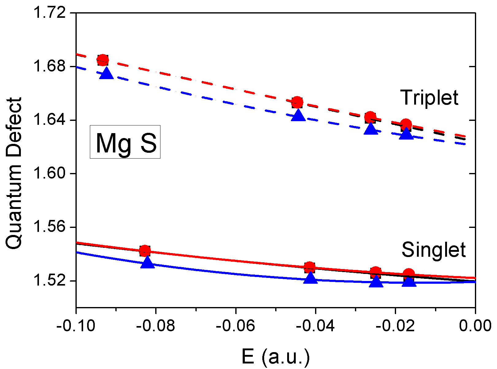
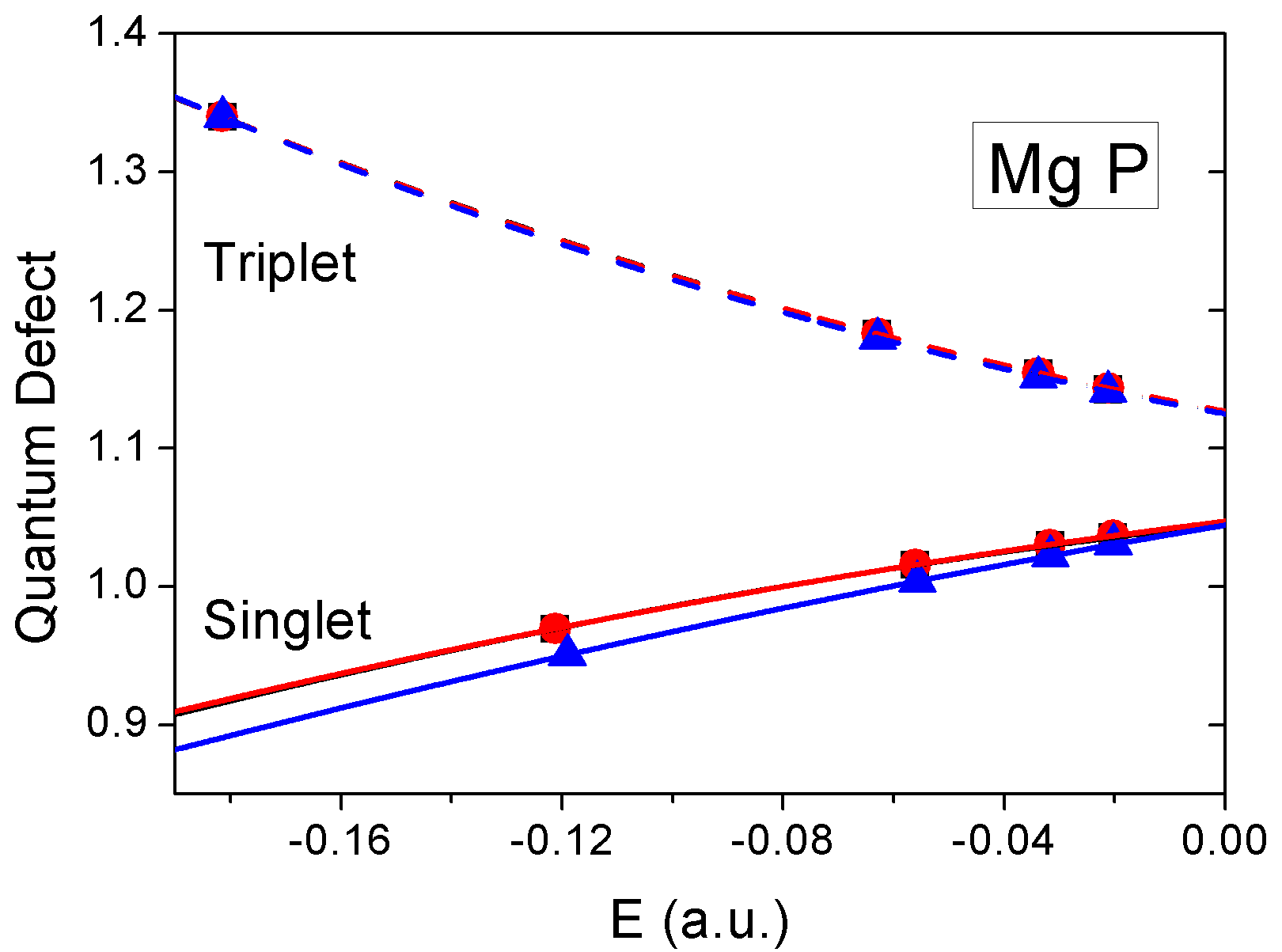
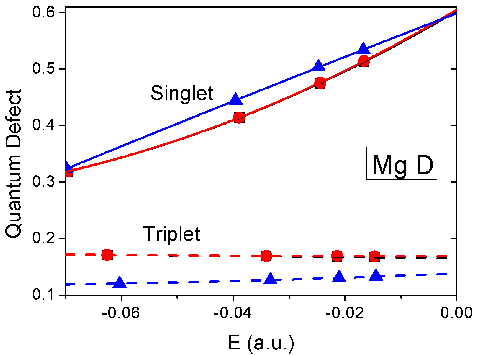
In Table 4, we give the parameters for all the different Rydberg series examined in this paper, using the experimental data. The first point to notice is the value of the QD at threshold. These vary from about 1.6 down to about -0.1. These dimensionless numbers are very important, as knowing only this value often yields a reasonably accurate Rydberg series, and also determines the scattering cross-section in the low-energy limitFWEZ07 . It is clear that our series cover a large range of different values for the QD.
| tr | Expt IP | Fit IP | ||||
|---|---|---|---|---|---|---|
| Be | ||||||
| 1S | 67.1 | -1.6 | 0.1 | 67.4 | -1.3 | 0.2 |
| 3S | 77.2 | -4.9 | -0.0 | 77.8 | -4.3 | 0.2 |
| 1P | 36.7 | 20.1 | -2.1 | 36.6 | 20.0 | -2.1 |
| 3P | 36.0 | -20.4 | 2.2 | 37.0 | -19.4 | 2.9 |
| 1D | -10.2 | 9.2 | -1.9 | -10.4 | 8.9 | -2.0 |
| 3D | 10.4 | -0.6 | -0.2 | 11.6 | 0.6 | 0.2 |
| MSE | 0.4 | 0.4 | 0.2 | |||
| MUE | 0.6 | 0.5 | 0.3 | |||
| Mg | ||||||
| 1S | 152.0 | -2.2 | 0.1 | 152.2 | -2.0 | 0.2 |
| 3S | 162.4 | -6.1 | 0.0 | 162.6 | -5.8 | 0.1 |
| 1P | 104.6 | 7.6 | -0.5 | 104.7 | 7.8 | -0.5 |
| 3P | 112.5 | -21.5 | 1.9 | 112.7 | -21.3 | 2.0 |
| 1D | 60.3 | 28.4 | 3.1 | 60.6 | 28.7 | 3.2 |
| 3D | 16.6 | -0.5 | 0.0 | 16.9 | -0.2 | 0.1 |
| MSE | 0.2 | 0.2 | 0.1 | |||
| MUE | 0.2 | 0.2 | 0.1 | |||
| Li | ||||||
| 2S | 39.6 | -0.7 | -0.1 | 39.9 | -0.5 | -0.0 |
| 2P | 4.5 | 0.5 | -0.1 | 4.7 | 0.6 | -0.0 |
| 2D | -0.2 | -0.3 | -0.1 | 0.1 | 0.0 | -0.0 |
| MSE | 0.3 | 0.3 | 0.1 | |||
| MUE | 0.3 | 0.3 | 0.1 | |||
Next, consider the values of . These can have either sign, meaning the QD can either increase or decrease with energy. The magnitude varies from almost 0 up to about 0.3. This gives the scale of the total change in the QD from the first transition to the threshold. Finally, we consider . These values are much smaller, never being larger than about 0.03, but also vary in sign. Thus this measure shows that the curvature has relatively little effect on the actual value of QD, and therefore on the Rydberg transition frequencies.
Now, we consider the values of the parameters that we found when the threshold energy was fitted rather than known from experiment. Typical errors introduced by the fitting procedure are about 0.004 or less. The only real outlier is the triplet D series in Be, where the threshold value is in error by 0.01. The curvature errors are typically even smaller (0.001), but since their values are already small, this appears as a greater fractional error. We conclude that errors on this scale will be introduced to QD parameters whenever IP’s are fit, as is done for all our pp calculations in the rest of this paper. Such errors are smaller than those made by the approximations we study below.
IV.3 Results for Be
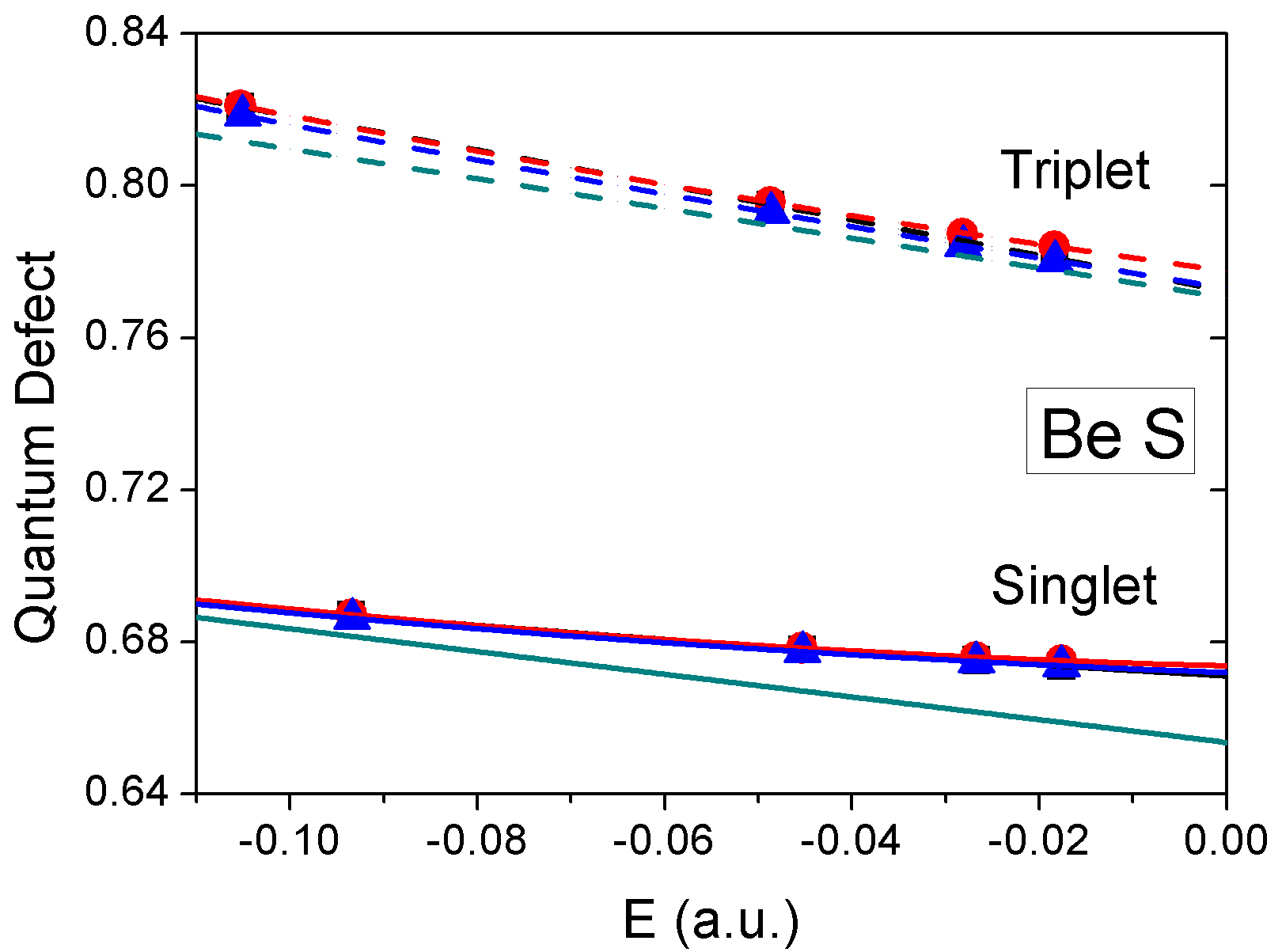
We begin the presentation of results with the simplest case: singlet and triplet S excitations in Be. We plot the experimental and pp-TDA results in Fig. 2, as well as the fit of TDLDA results on the exact ground-state KS potential from Ref. Faassen_2006_94102 . The figure shows several basic features. First, the difference between the black lines and red lines are almost invisible on this scale, showing that fitting the IP causes little degradation of results. Second, the pp blue lines are excellent approximations to the red lines, indicating that pp-TDA produces near perfect QDs for these series. Third, the TDDFT results (green) are quite good, especially for the triplet.
To quantify the differences in these curves, we extract , and from each curve in Tables 4 and 5, and compare the calculations with the experiment (with the exact IP). For both the triplet and singlet, the pp-TDA values are all excellent, and that even the curvature is within the error of the fit. The TDLDA results are almost as good (they were fit linearlyFaassen_2006_94102 , because the curvature is so small). However, there is a significant error in the TDLDA threshold value for the singlet, as is clearly visible in the figure, and the TDLDA slope is too large.
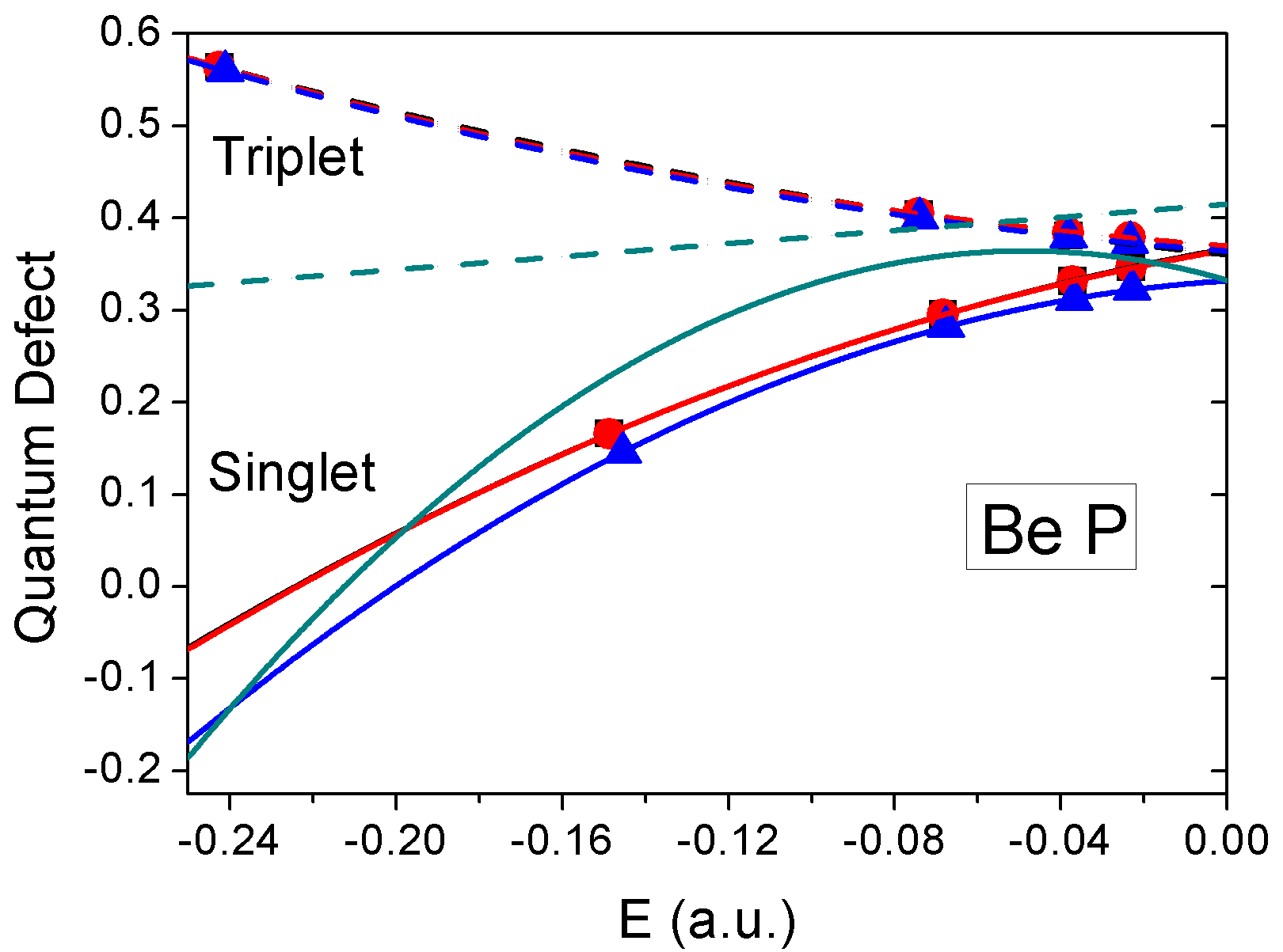
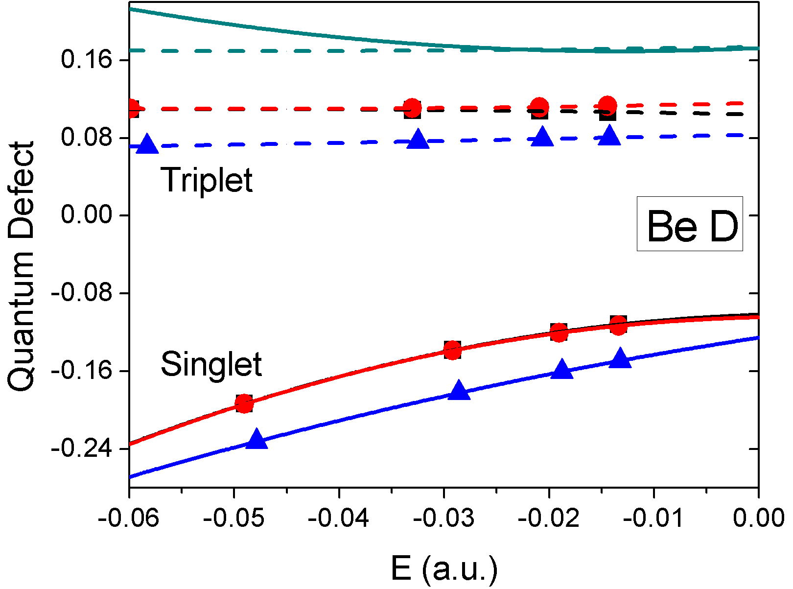
So, does pp-RPA always produce such excellent Rydberg series? In the next two figures, we repeat the procedure for the P and D series. In the P case, we see that the experimental QDs have substantially greater curvature than in the S series, especially for the singlet, and that pp-RPA captures this effect well. On the other hand, TDLDA is not working nearly as well, with the sign of being incorrect for the triplet, and the curvature being overestimated for the singlet.
The D QD has previously been noted as being challengingFaassen_2006_410 , and here TDLDA fails entirely. The TDLDA singlet/triplet ordering is wrong, and the threshold value is incorrect by more than 0.2. We see that although the pp-RPA results are less accurate than for S or P, they are still qualitatively and even quantitatively correct. The worst error is the threshold value for the triplet, being incorrect by 0.02, again, an order of magnitude better than TDLDA. For the Be D series, pp-RPA succeeds where TDLDA fails.
| tr. | pp | ALDA | ||||
|---|---|---|---|---|---|---|
| 1S | 67.2 | -1.4 | 0.1 | 65.4 | -2.8 | 0.0 |
| 3S | 77.3 | -4.5 | 0.1 | 77.1 | -4.1 | 0.0 |
| 1P | 33.2 | 18.6 | -3.7 | 33.3 | 12.4 | -8.2 |
| 3P | 36.4 | -19.6 | 2.8 | 41.5 | 9.0 | 0.0 |
| 1D | -12.5 | 10.7 | -0.7 | 17.3 | -5.0 | 2.1 |
| 3D | 8.3 | 1.2 | 0.00 | 17.4 | 0.4 | 0.2 |
| MSE | -1.2 | 0.5 | 0.1 | 5.8 | 1.3 | -0.7 |
| MUE | 1.4 | 1.0 | 0.6 | 7.5 | 9.0 | 2.1 |
Note that if a standard GGA or hybrid is used for the ground-state calculation, TDLDA will not produce a Rydberg series. Even methods designed to enforce the correct asymptotic behavior of the KS potential, such as the van Leeuwen-Baerends functional or asymptotically corrected methods, will typically produce terrible QDs. On the other hand, methods that include exact exchange (often denoted EXX) produce excellent KS potentials, whose performance will be comparable to that given here, since the small error in IP does not destroy the QD results when properly extracted. But none will do better than the results here, since we use the exact KS potential.
So, we can conclude that, for essentially every Be Rydberg series, pp-RPA outperforms TDLDA, even when TDLDA has been applied to the exact ground-state KS potential (and so the underlying IP is exactly right). While ALDA does remarkably well for such a low-cost calculation, it cannot compete with pp-RPA for accuracy.
IV.4 Results for Mg
| tr. | |||
|---|---|---|---|
| 1S | 151.9 | -1.4 | 0.5 |
| 3S | 162.1 | -5.3 | 0.4 |
| 1P | 104.5 | 9.4 | -0.3 |
| 3P | 112.5 | -21.5 | 2.2 |
| 1D | 59.9 | 27.6 | -0.2 |
| 3D | 13.8 | 1.8 | 0.2 |
| MSE | -0.6 | 0.8 | -0.3 |
| MUE | 0.6 | 1.1 | 0.8 |
To get an idea of how general this good performance of pp-RPA is, we repeat the calculations for Mg. In this case, the core is frozen leading to a substantial underestimate of the IP (0.13 eV) relative to experiment. Using the experimental IP with the pp transition frequencies would yield nonsensical QD values. But because our procedure fits this number, and then subsequent QD is plotted against the energy below threshold, we can see the the Mg QD results are typically almost (not quite) as good as those for Be. When averaging over all series, the Mg results are better than those of Be. This is a triumph of the QD method: Despite a substantial error in IP, the QD is still extractable and the underlying error in QD is very small.
IV.5 Results for an open shell
We finish our survey with an extreme challenge for pp-RPA. When the two-electron deficient reference is an unrestricted open-shell system, there are differences between and orbitals. The spin contamination and potential spin incompleteness usually cause both pp-RPA and pp-TDA to produce meaningless results. The Lithium atom is the simplest atoms with these problems.
With an -spin electron occupying the 1s orbital, the two-electron deficient reference for Li is hydrogenic. In principle, we can create a neutral doublet ground state by adding a electron to 1s and another electron to 2s, forming a state. But we could instead add two electrons to 1s and 2s separately to form the state. Since we can only perform unrestricted calculations with our program, both series of excitations are spin-contaminated. We denote the two series as AB and BB.
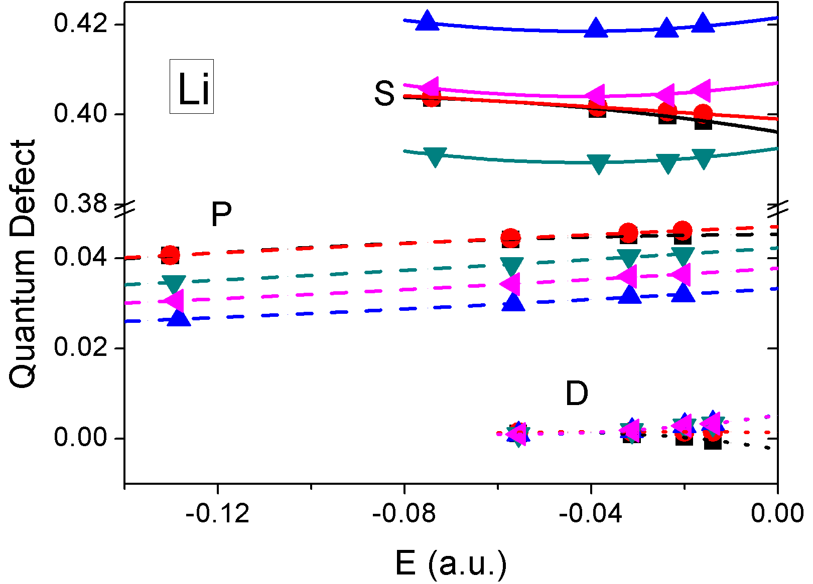
We can also attempt to overcome spin contamination by averaging these two, denoted AVE. We try all three ways to compute the doublet S, P, and D series of Li. We saw in Section IV.1 that, since AB overestimates the IP and BB underestimates it, their average has the most accurate IP, suggesting the AVE will yield the best results for the transition energies too.
The results of all three series are shown in figure 8. Note the -scale is much smaller than in previous figures, and the break in the curve. Overall, all three sets yield fairly accurate QD results, with MUE’s comparable to those for Be and Mg. For the S series, the AVE QD is substantially better than either AB or BB, while for the D series, the three are indistinguishable. But for the P series, the AVE curve is definitely worse than BB. So our QD analysis has shown that, although the AVE series always has the most accurate transition energy (because of its accurate IP), it does not always produce the best QD.
| tr. | AB | BB | AVE | ||||||
|---|---|---|---|---|---|---|---|---|---|
| 2S | 42.2 | 0.1 | 0.2 | 39.3 | 0.1 | 0.2 | 40.7 | 0.1 | 0.2 |
| 2P | 3.3 | 0.7 | 0.0 | 4.2 | 0.8 | 0.0 | 3.8 | 0.7 | 0.0 |
| 2D | 0.5 | 0.4 | 0.1 | 0.5 | 0.4 | 0.1 | 0.5 | 0.4 | 0.1 |
| MSE | 0.7 | 0.6 | 0.2 | 0.0 | 0.6 | 0.2 | 0.4 | 0.6 | 0.2 |
| MUE | 1.5 | 0.6 | 0.2 | 0.5 | 0.6 | 0.2 | 0.9 | 0.6 | 0.2 |
IV.6 Importance of pp reference state
The fact that pp-RPA and pp-TDA are able to describe charge transfer and Rydberg excitations is often attributed to their Coulomb and exchange kernels which are asymptotically correct. However, the orbital energies from the two-electron deficient reference also play a vital role. Although the Coulomb and exchange kernel is the same, the pp-RPA and pp-TDA with DFT references substantially underestimate the Rydberg excitation energies Yang_2013_224105 as a result of the poor Kohn-Sham orbital energies, making it meaningless to further look into the QD, just as in the TDDFT case. Because pp-RPA is only a first-order approximation to the adiabatic connection-pairing matrix fluctuation theory, it remains sensitive to the properties of the reference calculation. A well-behaved reference, such as HF in this atomic Rydberg excitation case, is needed for pp-RPA and pp-TDA to produce meaningful QDs. However, for low-energy excitations in molecules, DFT references lead to significantly better results.Yang_2014_124104
V Conclusion
In this paper, we have developed a very general approach for extracting both threshold energies and QDs from limited series of Rydberg excitations. We have demonstrated that our procedure can be used to extract extremely accurate threshold energies (errors in the 0.1 mH range), and maximum errors of order 0.01 for QDs. We have shown why measures like mean unsigned errors in collections of transition frequencies are not useful for Rydberg series, and how to parametrize and quantify errors in QD’s. We find that pp-RPA with a HF reference greatly outperforms TDDFT with a local approximation to the exchange-correlation kernel.
The results reported here should become the benchmark for approximate calculations of Rydberg series. Our QD extraction procedure can be applied to other series, such as excitions in solids. Any quantum chemical method for excitations should be measured against our pp-RPA results for these atoms. We suspect they will be difficult be beat with the same level of generality and low computational cost.
Acknowledgements.
Y.Y. appreciates the support as part of the Center for the Computational Design of Functional Layered Materials, an Energy Frontier Research Center funded by the U.S. Department of Energy, Office of Science, Basic Energy Sciences under Award DE-SC0012575. K.B. was supported by the U.S Department of Energy (DOE), Of- fice of Science, Basic Energy Sciences (BES) under award DE-FG02-08ER46496. W.Y. was supported by the National Science Foundation (CHE-1362927).References
- (1) E. Runge and E. K. U. Gross, Phys. Rev. Lett. 52, 997 (1984).
- (2) M. E. Casida, Time-dependent density functional response theory of molecular systems: Theory, computational methods, and functionals, in Recent Developments and Applications of Modern Density Functional Theory, edited by J. Seminario, volume 4 of Theoretical and Computational Chemistry, pages 391 – 439, Elsevier, 1996.
- (3) M. Petersilka, U. J. Gossmann, and E. K. U. Gross, Phys. Rev. Lett. 76, 1212 (1996).
- (4) C. Ullrich, Time-Dependent Density-Functional Theory: Concepts and Applications, Oxford Graduate Texts, OUP Oxford, 2012.
- (5) K. Burke, J. Werschnik, and E. K. U. Gross, The Journal of Chemical Physics 123, 062206 (2005).
- (6) D. J. Tozer and N. C. Handy, Phys. Chem. Chem. Phys. 2, 2117 (2000).
- (7) R. J. Cave, F. Zhang, N. T. Maitra, and K. Burke, Chemical Physics Letters 389, 39 (2004).
- (8) D. J. Tozer, R. D. Amos, N. C. Handy, B. O. Roos, and L. Serrano-Andres, Molecular Physics 97, 859 (1999).
- (9) A. Dreuw, J. L. Weisman, and M. Head-Gordon, The Journal of Chemical Physics 119, 2943 (2003).
- (10) A. Dreuw and M. Head-Gordon, Chemical Reviews 105, 4009 (2005).
- (11) T. Leininger, H. Stoll, H.-J. Werner, and A. Savin, Chemical Physics Letters 275, 151 (1997).
- (12) H. Iikura, T. Tsuneda, T. Yanai, and K. Hirao, The Journal of Chemical Physics 115, 3540 (2001).
- (13) R. van Leeuwen and E. J. Baerends, Phys. Rev. A 49, 2421 (1994).
- (14) D. J. Tozer and N. C. Handy, The Journal of Chemical Physics 109, 10180 (1998).
- (15) M. E. Casida and D. R. Salahub, The Journal of Chemical Physics 113, 8918 (2000).
- (16) Q. Wu, P. W. Ayers, and W. Yang, The Journal of Chemical Physics 119, 2978 (2003).
- (17) M. Seaton, Reports on Progress in Physics 46, 167 (1983).
- (18) M. van Faassen and K. Burke, The Journal of Chemical Physics 124, 094102 (2006).
- (19) A. Sommerfeld, Annalen der Physik 356, 1 (1916).
- (20) R. Guérout, M. Jungen, and C. Jungen, Journal of Physics B: Atomic, Molecular and Optical Physics 37, 3043 (2004).
- (21) R. Guérout, M. Jungen, and C. Jungen, Journal of Physics B: Atomic, Molecular and Optical Physics 37, 3057 (2004).
- (22) I. D. Petsalakis, G. Theodorakopoulos, and R. J. Buenker, Journal of Chemical Physics 119, 2004 (2003).
- (23) F. Merkt, Annual Review of Physical Chemistry 48, 675 (1997), PMID: 15012453.
- (24) G. Herzberg, Annual review of physical chemistry 38, 27 (1987).
- (25) M. van Faassen and K. Burke, Phys. Chem. Chem. Phys. 11, 4437 (2009).
- (26) A. Wasserman and K. Burke, Phys. Rev. Lett. 95, 163006 (2005).
- (27) M. van Faassen and K. Burke, Chemical Physics Letters 431, 410 (2006).
- (28) Y. Yang, H. van Aggelen, and W. Yang, The Journal of Chemical Physics 139, 224105 (2013).
- (29) Y. Yang, D. Peng, J. Lu, and W. Yang, The Journal of Chemical Physics 141, 124104 (2014).
- (30) Y. Yang, D. Peng, E. R. Davidson, and W. Yang, The Journal of Physical Chemistry A 119, 4923 (2015), PMID: 25891638.
- (31) H. van Aggelen, Y. Yang, and W. Yang, Phys. Rev. A 88, 030501 (2013).
- (32) H. van Aggelen, Y. Yang, and W. Yang, The Journal of Chemical Physics 140, 18A511 (2014).
- (33) D. J. Rowe, Rev. Mod. Phys. 40, 153 (1968).
- (34) P. Ring and P. Schuck, The Nuclear Many-Body Problem, Physics and astronomy online library, Springer, 2004.
- (35) Y. Yang, H. van Aggelen, S. N. Steinmann, D. Peng, and W. Yang, The Journal of Chemical Physics 139, 174110 (2013).
- (36) D. Peng, H. van Aggelen, Y. Yang, and W. Yang, The Journal of Chemical Physics 140, 18A522 (2014).
- (37) T. Helgaker, P. Jørgensen, and J. Olsen, Molecular electronic-structure theory, Wiley, 2000.
- (38) Q. Wu, A. J. Cohen, and W. Yang, Molecular Physics 103, 711 (2005).
- (39) An in-house program for QM/MM simulations (http://www.qm4d.info).
- (40) A. E. Kramida, Y. Ralchenko, J. Reader, and N. A. Team, NIST Atomic Spectra Database (version 5.0), 2012.
- (41) M. van Faassen, A. Wasserman, E. Engel, F. Zhang, and K. Burke, Phys. Rev. Lett. 99, 043005 (2007).