Binary Rate Distortion With Side Information:
The Asymmetric Correlation Channel Case

Andrei Sechelea1, Samuel Cheng2, Adrian Munteanu1, and Nikos Deligiannis1
E-mail: {atsechel, acmuntea, ndeligia}@etro.vub.ac.be, samuel.cheng@ou.edu
1Department of Electronics and Informatics, Vrije Universiteit Brussel, Brussels, Belgium 2School of Electrical and Computer Engineering, University of Oklahoma, Tulsa, OK USA
Abstract

Advancing over up-to-date information theoretic results that assume symmetric correlation models, in this work we consider the problem of lossy binary source coding with side information, where the correlation is expressed by a generic binary asymmetric channel. Specifically, we present an in-depth analysis of rate distortion with side information available to both the encoder and decoder (conventional predictive), as well as the Wyner-Ziv problem for this particular setup. Prompted by our recent results for the Z-channel correlation case, we evaluate the rate loss between the Wyner-Ziv and the conventional predictive coding, as a function of the parameters of the binary asymmetric correlation channel.

Index Terms:
Source coding with side information, Wyner-Ziv coding, rate-distortion bound, asymmetric channel

I Introduction

Using side information is fundamental in many source and channel coding problems and has recently been adopted in new fields, like compressed sensing and compressive classification [1]. The vast majority of results in discrete source coding with side information assume that correlation channel between the source and the side information to be symmetric. Side information is also a key factor in distributed source coding; e.g. recent results in distributed video coding [2, 3] have shown that using an asymmetric channel model to express the correlation between the source (frame to be encoded) and the side information (motion-compensated prediction) leads to substantial compression performance gains compared to the case where a conventional symmetric correlation channel model is used.

In this work, we focus on the theory of rate distortion with side information. Specifically, we consider the following setup: let (X,Y)βˆˆπ’³Γ—π’΄π‘‹π‘Œπ’³π’΄(X,Y)\in\mathcal{X}\times\mathcal{Y} be correlated binary random variables, such that the source X∽Bernoulli​(0.5)βˆ½π‘‹Bernoulli0.5X\backsim\textit{Bernoulli}(0.5) is to be encoded using the source Yπ‘ŒY as side information. The correlation between the two sources is described by a binary asymmetric channel:

p​(Y|X)=[(1βˆ’a)ab(1βˆ’b)],𝑝conditionalπ‘Œπ‘‹matrix1π‘Žπ‘Žπ‘1𝑏p(Y|X)=\begin{bmatrix}(1-a)&a\\ b&(1-b)\end{bmatrix}, (1)

(a,b)∈[0,1]2π‘Žπ‘superscript012(a,b)\in\big{[}0,1\big{]}^{2}. The reconstructed source is the binary variable X^βˆˆπ’³^^𝑋^𝒳\hat{X}\in\hat{\mathcal{X}}, and the distortion metric considered is the Hamming distance: if (x,x^)βˆˆπ’³Γ—π’³^π‘₯^π‘₯𝒳^𝒳(x,\hat{x})\in\mathcal{X}\times\hat{\mathcal{X}} then dH​(x,x^)=0subscript𝑑𝐻π‘₯^π‘₯0d_{H}(x,\hat{x})=0 if x=x^π‘₯^π‘₯x=\hat{x}, and dH​(x,x^)=1subscript𝑑𝐻π‘₯^π‘₯1d_{H}(x,\hat{x})=1 if xβ‰ x^π‘₯^π‘₯x\neq\hat{x}. Our goal is to describe the rate distortion characteristics of this system in two cases, that is when the side information Yπ‘ŒY is available at (i) both the encoder and decoder, corresponding to the conventional predictive case, and (ii) available only at the decoder, i.e., the Wyner-Ziv (WZ) case.

For the binary symmetric correlation, the rate distortion functions were given by Berger in [4] for the predictive case, and respectively by Wyner and Ziv in [5], for the corresponding WZ case. Another binary correlation channel that has been recently studied is the Z-channel, for which Steinberg derived in [6] the rate distortion bound RX|YZ​(d)superscriptsubscript𝑅conditionalπ‘‹π‘Œπ‘π‘‘R_{X|Y}^{Z}(d) for the predictive case, while in [7] we derived the rate distortion bound RW​ZZ​(d)superscriptsubscriptπ‘…π‘Šπ‘π‘π‘‘R_{WZ}^{Z}(d) for the Wyner-Ziv case. In [5], it is established that, for the general case, a rate loss exists between the predictive and WZ bounds. Zamir showed in [8] that, for binary sources and the Hamming distortion metric, the rate loss is at most 0.22 bits/sample, and in [7] we show that this difference vanishes in the case of the Z-channel correlation.

To the best of our knowledge, the characterization of the binary rate distortion function in the general case of the asymmetric correlation is still an open problem. A straightforward option is to use a numerical algorithm to compute it, such as the Blahut-Arimoto [9] implementation in [10]. Unfortunately, such a numerical analysis does not provide an analytical characterization of the rate distortion function nor an understanding of its behaviour in various rate regions.

In this paper, we present the derivation of the conventional predictive RX|Y​(d)subscript𝑅conditionalπ‘‹π‘Œπ‘‘R_{X|Y}(d) function for the considered setup. Subsequently, by considering a binary auxiliary variable in the formulations of [5], we derive rate and distortion expressions that yield a bound for the WZ problem. Furthermore, through our analysis, we are able to evaluate the evolution of the rate-loss, with respect to the crossover probabilities of the binary asymmetric correlation channel.

II Source coding with Encoder-Decoder Side Information

When the side information is available both at the encoder and the decoder, the rate-distortion function is given by

RX|Y​(d)=infp​(x^|x,y):E​[d​(X,X^)]≀dI​(X;X^|Y),subscript𝑅conditionalπ‘‹π‘Œπ‘‘subscriptinfimum:𝑝conditional^π‘₯π‘₯𝑦𝐸delimited-[]𝑑𝑋^𝑋𝑑𝐼𝑋conditional^π‘‹π‘ŒR_{X|Y}(d)=\inf_{p(\hat{x}|x,y):\ E\big{[}d(X,\hat{X})\big{]}\leq d}I(X;\hat{X}|Y), (2)

where E​[β‹…]𝐸delimited-[]β‹…E\big{[}\cdot\big{]} denotes the expectation operator and d𝑑d is the targeted distortion.

The quantity to be minimized in (2) can be written as

I​(X;X^|Y)𝐼𝑋conditional^π‘‹π‘Œ\displaystyle I(X;\hat{X}|Y) =H​(X|Y)βˆ’H​(X|X^,Y)absent𝐻conditionalπ‘‹π‘Œπ»conditional𝑋^π‘‹π‘Œ\displaystyle=\ H(X|Y)-H(X|\hat{X},Y)
=H​(X|Y)βˆ’H​(XβŠ•X^|X^,Y)absent𝐻conditionalπ‘‹π‘Œπ»direct-sum𝑋conditional^𝑋^π‘‹π‘Œ\displaystyle=\ H(X|Y)-H(X\oplus\hat{X}|\hat{X},Y)
β‰₯H​(X|Y)βˆ’H​(π’Ÿ|Y),absent𝐻conditionalπ‘‹π‘Œπ»conditionalπ’Ÿπ‘Œ\displaystyle\geq H(X|Y)-H(\mathcal{D}|Y), (3)

where H​(β‹…)𝐻⋅H(\cdot) denotes the binary entropy function and π’Ÿ=XβŠ•X^π’Ÿdirect-sum𝑋^𝑋\mathcal{D}=X\oplus\hat{X}. With the Xβˆ’Yπ‘‹π‘ŒX-Y correlation channel given by (1), the maximum distortion to be considered is the average crossover of the side information channel, i.e., if X^=Y^π‘‹π‘Œ\hat{X}=Y: Dm​a​x=a+b2subscriptπ·π‘šπ‘Žπ‘₯π‘Žπ‘2D_{max}=\frac{a+b}{2}. We consider the inverse channel Yβˆ’Xπ‘Œπ‘‹Y-X:

p​(X|Y)𝑝conditionalπ‘‹π‘Œ\displaystyle p(X|Y) =[1βˆ’aβˆ—aβˆ—bβˆ—1βˆ’bβˆ—]absentmatrix1superscriptπ‘Žsuperscriptπ‘Žsuperscript𝑏1superscript𝑏\displaystyle=\begin{bmatrix}1-a^{*}&a^{*}\\ b^{*}&1-b^{*}\end{bmatrix}\ =[(1βˆ’a)1βˆ’a+bb1βˆ’a+baa+1βˆ’b(1βˆ’b)a+1βˆ’b].absentmatrix1π‘Ž1π‘Žπ‘π‘1π‘Žπ‘π‘Žπ‘Ž1𝑏1π‘π‘Ž1𝑏\displaystyle=\begin{bmatrix}\frac{(1-a)}{1-a+b}&\frac{b}{1-a+b}\\ \frac{a}{a+1-b}&\frac{(1-b)}{a+1-b}\end{bmatrix}. (4)

We have p​(Y=0)=1βˆ’a+b2π‘π‘Œ01π‘Žπ‘2p(Y=0)=\frac{1-a+b}{2} and p​(Y=1)=a+1βˆ’b2π‘π‘Œ1π‘Ž1𝑏2p(Y=1)=\frac{a+1-b}{2}, and the maximum distortion can be written as Dm​a​x=p​(Y=0)β‹…aβˆ—+p​(Y=1)β‹…bβˆ—subscriptπ·π‘šπ‘Žπ‘₯β‹…π‘π‘Œ0superscriptπ‘Žβ‹…π‘π‘Œ1superscript𝑏D_{max}=p(Y=0)\cdot a^{*}+p(Y=1)\cdot b^{*}. Without loss of generality, let a≀bπ‘Žπ‘a\leq b in (1). This implies aβˆ—β‰₯bβˆ—superscriptπ‘Žsuperscript𝑏a^{*}\geq b^{*}. Given that the side information is known at the encoder, we can always describe the overall distortion as being

d=E​[π’Ÿ]=p​(Y=0)β‹…dY=0+p​(Y=1)β‹…dY=1,𝑑𝐸delimited-[]π’Ÿβ‹…π‘π‘Œ0subscriptπ‘‘π‘Œ0β‹…π‘π‘Œ1subscriptπ‘‘π‘Œ1d=E\big{[}\mathcal{D}\big{]}=p(Y=0)\cdot d_{Y=0}+p(Y=1)\cdot d_{Y=1}, (5)

where dY=0=E​[d​(X,X^)|Y=0]≀aβˆ—subscriptπ‘‘π‘Œ0𝐸delimited-[]conditional𝑑𝑋^π‘‹π‘Œ0superscriptπ‘Žd_{Y=0}=E\big{[}d(X,\hat{X})|Y=0\big{]}\leq a^{*} and dY=1=E​[d​(X,X^)|Y=1]≀bβˆ—subscriptπ‘‘π‘Œ1𝐸delimited-[]conditional𝑑𝑋^π‘‹π‘Œ1superscript𝑏d_{Y=1}=E\big{[}d(X,\hat{X})|Y=1\big{]}\leq b^{*}.

Maximizing the term H​(π’Ÿ|Y)𝐻conditionalπ’Ÿπ‘ŒH(\mathcal{D}|Y) in (3) with the above mentioned constraints gives the minimum for I​(X;X^|Y)𝐼𝑋conditional^π‘‹π‘ŒI(X;\hat{X}|Y). This is an optimization problem that can be expressed using the Karush-Kuhn-Tucker conditions:

maximize p​(Y=0)β‹…H​(dY=0)+p​(Y=1)β‹…H​(dY=1)β‹…π‘π‘Œ0𝐻subscriptπ‘‘π‘Œ0β‹…π‘π‘Œ1𝐻subscriptπ‘‘π‘Œ1\displaystyle p(Y=0)\cdot H(d_{Y=0})+p(Y=1)\cdot H(d_{Y=1})
subject to {p​(Y=0)β‹…dY=0+p​(Y=1)β‹…dY=1=ddY=0≀aβˆ—dY=1≀bβˆ—casesβ‹…π‘π‘Œ0subscriptπ‘‘π‘Œ0β‹…π‘π‘Œ1subscriptπ‘‘π‘Œ1𝑑otherwisesubscriptπ‘‘π‘Œ0superscriptπ‘Žotherwisesubscriptπ‘‘π‘Œ1superscript𝑏otherwise\displaystyle\begin{cases}p(Y=0)\cdot d_{Y=0}+p(Y=1)\cdot d_{Y=1}=d\\ d_{Y=0}\leq a^{*}\\ d_{Y=1}\leq b^{*}\end{cases} (6)

We formulate the Lagrangian optimization problem with the above inequality constraints, and the Lagrangian function is:

π’₯=p​(Y=0)β‹…H​(dY=0)+p​(Y=1)β‹…H​(dY=1)+λ​(p​(Y=0)β‹…dY=0+p​(Y=1)β‹…dY=1βˆ’d)+Ξ»0​(dY=0βˆ’aβˆ—)+Ξ»1​(dY=1βˆ’bβˆ—)π’₯β‹…π‘π‘Œ0𝐻subscriptπ‘‘π‘Œ0β‹…π‘π‘Œ1𝐻subscriptπ‘‘π‘Œ1πœ†β‹…π‘π‘Œ0subscriptπ‘‘π‘Œ0β‹…π‘π‘Œ1subscriptπ‘‘π‘Œ1𝑑subscriptπœ†0subscriptπ‘‘π‘Œ0superscriptπ‘Žsubscriptπœ†1subscriptπ‘‘π‘Œ1superscript𝑏\begin{split}\mathcal{J}=p(Y=0)\cdot H(d_{Y=0})+p(Y=1)\cdot H(d_{Y=1})+\\ \lambda(p(Y=0)\cdot d_{Y=0}+p(Y=1)\cdot d_{Y=1}-d)+\\ \lambda_{0}(d_{Y=0}-a^{*})+\lambda_{1}(d_{Y=1}-b^{*})\end{split} (7)

Deriving with respect to the unknowns yields:

RX|Y​(d)={p​(Y=0)β‹…[H​(aβˆ—)βˆ’H​(d)]+p​(Y=1)β‹…[H​(bβˆ—)βˆ’H​(d)],if​d≀bβˆ—p​(Y=0)β‹…[H​(aβˆ—)βˆ’H​(dβˆ’a2p​(Y=0))],if​bβˆ—β‰€d≀Dm​a​x0,if​dβ‰₯Dm​a​xsubscript𝑅conditionalπ‘‹π‘Œπ‘‘caseslimit-fromβ‹…π‘π‘Œ0delimited-[]𝐻superscriptπ‘Žπ»π‘‘otherwiseβ‹…π‘π‘Œ1delimited-[]𝐻superscript𝑏𝐻𝑑if𝑑superscript𝑏otherwiseβ‹…π‘π‘Œ0delimited-[]𝐻superscriptπ‘Žπ»π‘‘π‘Ž2π‘π‘Œ0otherwiseifsuperscript𝑏𝑑subscriptπ·π‘šπ‘Žπ‘₯otherwise0if𝑑subscriptπ·π‘šπ‘Žπ‘₯otherwiseR_{X|Y}(d)=\begin{cases}p(Y=0)\cdot\big{[}H(a^{*})-H(d)\big{]}+\\ \qquad p(Y=1)\cdot\big{[}H(b^{*})-H(d)\big{]},\ \ \mbox{if}\ d\leq b^{*}\\ p(Y=0)\cdot\big{[}H(a^{*})-H(\frac{d-\frac{a}{2}}{p(Y=0)})\big{]},\\ \qquad\ \ \ \mbox{if}\ b^{*}\leq d\leq D_{max}\\ 0,\qquad\mbox{if}\ d\geq D_{max}\end{cases} (8)

This can be achieved by considering an auxiliary variable Uπ‘ˆU given by a binary symmetric channel with input X𝑋X and output Uπ‘ˆU, with crossover probability p0subscript𝑝0p_{0} as follows:

p0={if​d≀bβˆ—then​p0=dif​d>bβˆ—then​p0=dβˆ’p​(Y=1)β‹…bβˆ—p​(Y=0)subscript𝑝0casesif𝑑superscript𝑏thensubscript𝑝0𝑑if𝑑superscript𝑏thensubscript𝑝0π‘‘β‹…π‘π‘Œ1superscriptπ‘π‘π‘Œ0p_{0}=\begin{cases}\mbox{if}\ d\leq b^{*}&\mbox{then}\ p_{0}=d\\ \mbox{if}\ d>b^{*}&\mbox{then}\ p_{0}=\frac{d-p(Y=1)\cdot b^{*}}{p(Y=0)}\end{cases} (9)

The corresponding reconstruction function is:

{if​d≀bβˆ—then​X^=Uif​d>bβˆ—then​{X^=Yif​Y=1X^=Uif​Y=0casesif𝑑superscript𝑏then^π‘‹π‘ˆif𝑑superscript𝑏thencases^π‘‹π‘Œifπ‘Œ1^π‘‹π‘ˆifπ‘Œ0\begin{cases}\mbox{if}\ d\leq b^{*}&\mbox{then}\ \hat{X}=U\\ \mbox{if}\ d>b^{*}&\mbox{then}\ \begin{cases}\hat{X}=Y&\mbox{if}\ Y=1\\ \hat{X}=U&\mbox{if}\ Y=0\end{cases}\end{cases} (10)

III Source Coding with Side Information at the Decoder

When the side information is available only at the decoder, the R-D function is given by

RW​Z​(d)=infp​(u|x)​p​(x^|u,y):E​[d​(X,X^)]≀dI​(X;U|Y),subscriptπ‘…π‘Šπ‘π‘‘subscriptinfimum:𝑝conditional𝑒π‘₯𝑝conditional^π‘₯𝑒𝑦𝐸delimited-[]𝑑𝑋^𝑋𝑑𝐼𝑋conditionalπ‘ˆπ‘ŒR_{WZ}(d)=\inf_{p(u|x)p(\hat{x}|u,y):\ E[d(X,\hat{X})]\leq d}I(X;U|Y), (11)

where X^=f​(U,Y)^π‘‹π‘“π‘ˆπ‘Œ\hat{X}=f(U,Y) and Uπ‘ˆU is an auxiliary random variable, satisfying the Markov chains: U↔X↔Yβ†”π‘ˆπ‘‹β†”π‘ŒU\leftrightarrow X\leftrightarrow Y and X↔(U,Y)↔X^β†”π‘‹π‘ˆπ‘Œβ†”^𝑋X\leftrightarrow(U,Y)\leftrightarrow\hat{X}, such that E​[d​(X,X^)]≀d𝐸delimited-[]𝑑𝑋^𝑋𝑑E\big{[}d(X,\hat{X})\big{]}\leq d. Let Uβˆˆπ’°π‘ˆπ’°U\in\mathcal{U} be the outcome obtained from a binary channel with input X𝑋X and the transition matrix given by:

p​(U|X)=[(1βˆ’p)pq(1βˆ’q)],𝑝conditionalπ‘ˆπ‘‹matrix1π‘π‘π‘ž1π‘žp(U|X)=\begin{bmatrix}(1-p)&p\\ q&(1-q)\end{bmatrix}, (12)

with (p,q)∈[0,1]2π‘π‘žsuperscript012(p,q)\in\big{[}0,1\big{]}^{2}.

We will express the resulting rate and distortion as functions of the crossover probabilities of the channels in (1) and (12).

III-A Expression of the Rate

The quantity to be minimized in (11) is written as

I​(X;U|Y)=H​(U|Y)βˆ’H​(U|X).𝐼𝑋conditionalπ‘ˆπ‘Œπ»conditionalπ‘ˆπ‘Œπ»conditionalπ‘ˆπ‘‹I(X;U|Y)=H(U|Y)-H(U|X). (13)

Given the Markovianity U↔X↔Yβ†”π‘ˆπ‘‹β†”π‘ŒU\leftrightarrow X\leftrightarrow Y the channel between Yπ‘ŒY and Uπ‘ˆU can be expressed as the concatenation of the channels Xβˆ’Uπ‘‹π‘ˆX-U and Xβˆ’Yπ‘‹π‘ŒX-Y. Knowing (4) and (12) the transition matrix is

p​(U|Y)𝑝conditionalπ‘ˆπ‘Œ\displaystyle p(U|Y) =[(1βˆ’a)​(1βˆ’p)+b​q1βˆ’a+b(1βˆ’a)​p+b​(1βˆ’q)1βˆ’a+ba​(1βˆ’p)+(1βˆ’b)​qa+1βˆ’ba​p+(1βˆ’b)​(1βˆ’q)a+1βˆ’b].absentmatrix1π‘Ž1π‘π‘π‘ž1π‘Žπ‘1π‘Žπ‘π‘1π‘ž1π‘Žπ‘π‘Ž1𝑝1π‘π‘žπ‘Ž1π‘π‘Žπ‘1𝑏1π‘žπ‘Ž1𝑏\displaystyle=\begin{bmatrix}\frac{(1-a)(1-p)+bq}{1-a+b}&\frac{(1-a)p+b(1-q)}{1-a+b}\\ \frac{a(1-p)+(1-b)q}{a+1-b}&\frac{ap+(1-b)(1-q)}{a+1-b}\end{bmatrix}. (14)

Therefore, based on (13), let us define RW​Zβˆ—β€‹(p,q)superscriptsubscriptπ‘…π‘Šπ‘π‘π‘žR_{WZ}^{*}(p,q) to be:

I​(X;U|Y)𝐼𝑋conditionalπ‘ˆπ‘Œ\displaystyle I(X;U|Y) β‰œRW​Zβˆ—β€‹(p,q)=H​(U|Y)βˆ’H​(U|X)β‰œabsentsuperscriptsubscriptπ‘…π‘Šπ‘π‘π‘žπ»conditionalπ‘ˆπ‘Œπ»conditionalπ‘ˆπ‘‹\displaystyle\triangleq\ R_{WZ}^{*}(p,q)=H(U|Y)-H(U|X)
=(1βˆ’a+b)2β‹…H​((1βˆ’a)​(1βˆ’p)+b​q1βˆ’a+b)absentβ‹…1π‘Žπ‘2𝐻1π‘Ž1π‘π‘π‘ž1π‘Žπ‘\displaystyle=\frac{(1-a+b)}{2}\cdot H\left(\frac{(1-a)(1-p)+bq}{1-a+b}\right)
+(a+1βˆ’b)2β‹…H​(a​(1βˆ’p)+(1βˆ’b)​qa+1βˆ’b)β‹…π‘Ž1𝑏2π»π‘Ž1𝑝1π‘π‘žπ‘Ž1𝑏\displaystyle+\frac{(a+1-b)}{2}\cdot H\left(\frac{a(1-p)+(1-b)q}{a+1-b}\right)
βˆ’12β‹…[H​(p)+H​(q)].β‹…12delimited-[]π»π‘π»π‘ž\displaystyle\qquad\qquad\qquad-\frac{1}{2}\cdot\big{[}H(p)+\ H(q)\big{]}. (15)

III-B Expression of the Distortion

The distortion expression can be determined by observing that for a fixed pair (u,y)𝑒𝑦(u,y), xπ‘₯x is given by the conditional distribution p​(x|u,y)𝑝conditionalπ‘₯𝑒𝑦p(x|u,y). Since the decoder can only make a deterministic decision given u𝑒u and y𝑦y, the best choice is to output:

x^=f​(u,y)=arg​maxx⁑p​(x|u,y).^π‘₯𝑓𝑒𝑦subscriptargmaxπ‘₯𝑝conditionalπ‘₯𝑒𝑦\hat{x}=f(u,y)=\operatorname*{arg\,max}_{x}p(x|u,y). (16)

We can write the error rate conditioned on (u,y)𝑒𝑦(u,y) as [1βˆ’p​(f​(u,y)|u,y)]delimited-[]1𝑝conditional𝑓𝑒𝑦𝑒𝑦\big{[}1-p(f(u,y)|u,y)\big{]}, so the average distortion is given by

d=βˆ‘u,y(1βˆ’p​(f​(u,y)|u,y))​p​(u,y).𝑑subscript𝑒𝑦1𝑝conditional𝑓𝑒𝑦𝑒𝑦𝑝𝑒𝑦d=\sum_{u,y}(1-p(f(u,y)|u,y))p(u,y). (17)

This is equivalent to:

d=βˆ‘u,ymin⁑(p​(X=0,y,u),p​(X=1,y,u)).𝑑subscript𝑒𝑦𝑝𝑋0𝑦𝑒𝑝𝑋1𝑦𝑒d=\sum_{u,y}\min(\ p(X=0,y,u),\ p(X=1,y,u)\ ). (18)

Knowing that, due to the Markov property U↔X↔Yβ†”π‘ˆπ‘‹β†”π‘ŒU\leftrightarrow X\leftrightarrow Y,

p​(x,y,u)=p​(x,y)​p​(u|x)=p​(x)​p​(y|x)​p​(u|x)𝑝π‘₯𝑦𝑒𝑝π‘₯𝑦𝑝conditional𝑒π‘₯𝑝π‘₯𝑝conditional𝑦π‘₯𝑝conditional𝑒π‘₯p(x,y,u)=p(x,y)p(u|x)=p(x)p(y|x)p(u|x) (19)

we can write p​(x,y,u)𝑝π‘₯𝑦𝑒p(x,y,u) as follows:

p​(X=0,Y,U)=12β‹…[(1βˆ’a)​(1βˆ’p)(1βˆ’a)​pa​(1βˆ’p)a​p],𝑝𝑋0π‘Œπ‘ˆβ‹…12matrix1π‘Ž1𝑝1π‘Žπ‘π‘Ž1π‘π‘Žπ‘p(X=0,Y,U)=\frac{1}{2}\cdot\begin{bmatrix}(1-a)(1-p)&(1-a)p\\ a(1-p)&ap\end{bmatrix}, (20)

and

p​(X=1,Y,U)=12β‹…[b​qb​(1βˆ’q)(1βˆ’b)​q(1βˆ’b)​(1βˆ’q)].𝑝𝑋1π‘Œπ‘ˆβ‹…12matrixπ‘π‘žπ‘1π‘ž1π‘π‘ž1𝑏1π‘žp(X=1,Y,U)=\frac{1}{2}\cdot\begin{bmatrix}bq&b(1-q)\\ (1-b)q&(1-b)(1-q)\end{bmatrix}. (21)

At this point, it is useful to make the following observations regarding the symmetries of the RW​Zβˆ—β€‹(p,q)superscriptsubscriptπ‘…π‘Šπ‘π‘π‘žR_{WZ}^{*}(p,q) and d𝑑d with respect to the crossover probabilities in (1) and (12):

  • β€’

    If in (1) we substitute the pair (a,b)π‘Žπ‘(a,b) by (1βˆ’a,1βˆ’b)1π‘Ž1𝑏(1-a,1-b), the functions RW​Zβˆ—β€‹(p,q)superscriptsubscriptπ‘…π‘Šπ‘π‘π‘žR_{WZ}^{*}(p,q) and d𝑑d do not change.

  • β€’

    If in (12) we substitute the pair (p,q)π‘π‘ž(p,q) by (1βˆ’p,1βˆ’q)1𝑝1π‘ž(1-p,1-q), the functions RW​Zβˆ—β€‹(p,q)superscriptsubscriptπ‘…π‘Šπ‘π‘π‘žR_{WZ}^{*}(p,q) and d𝑑d do not change.

Essentially, the substitutions are equivalent to a label swap at the output of the respective channels and do not affect the rate-distortion function. The consequence is that the domains of interest for the pairs (a,b)π‘Žπ‘(a,b) and (p,q)π‘π‘ž(p,q) can be reduced from [0,1]2superscript012[0,1]^{2} to 0≀a+b≀10π‘Žπ‘10\leq a+b\leq 1 and 0≀p+q≀10π‘π‘ž10\leq p+q\leq 1. Using symmetry constraints and (20), (21), equation (18) becomes:

π’Ÿβ€‹(p,q)=π’Ÿπ‘π‘žabsent\displaystyle\mathcal{D}(p,q)= (bq+min((1βˆ’a)p,b(1βˆ’q))+\displaystyle(bq+\min((1-a)p,b(1-q))+
min(a(1βˆ’p),(1βˆ’b)q)+ap)/2.\displaystyle\min(a(1-p),(1-b)q)+ap)/2. (22)

There can be four possible expressions for the above equation, each corresponding to a different reconstruction strategy at the decoder. Without loss of generality, let a<bπ‘Žπ‘a<b, fixed by the initial setup. The crossover probabilities p𝑝p and qπ‘žq can vary.

In order to emphasize the decision taken by the reconstruction function given in (16) for every pair (y,u)𝑦𝑒(y,u), we introduce the following function:

x^o​u​t(y,u)=arg​maxxp(x,Y=y,U=u)\hat{x}_{out}(y,u)=\operatorname*{arg\,max}_{x}p(x,Y=y,U=u) (23)

In our binary case, x^o​u​tsubscript^π‘₯π‘œπ‘’π‘‘\hat{x}_{out} can be seen a 2Γ—2222\times 2 matrix, with the lines corresponding to the values of Y∈{0,1}π‘Œ01Y\in\{0,1\}, and columns corresponding to the values of U∈{0,1}π‘ˆ01U\in\{0,1\}, indicating whether the reconstruction was x^=0^π‘₯0\hat{x}=0 or x^=1^π‘₯1\hat{x}=1.

The possible expressions for (22) are the following:

  • β€’

    when {(1βˆ’a)​p<b​(1βˆ’q)a​(1βˆ’p)>(1βˆ’b)​q,cases1π‘Žπ‘π‘1π‘žotherwiseπ‘Ž1𝑝1π‘π‘žotherwise\begin{cases}(1-a)p<b(1-q)\\ a(1-p)>(1-b)q\end{cases}, x^o​u​t=(0101)subscript^π‘₯π‘œπ‘’π‘‘0101\hat{x}_{out}=\left(\begin{array}[]{cc}0&1\\ 0&1\end{array}\right) is equivalent to having the reconstruction function X^=U^π‘‹π‘ˆ\hat{X}=U and a distortion value of D1=p+q2subscript𝐷1π‘π‘ž2D_{1}=\frac{p+q}{2};

  • β€’

    when {(1βˆ’a)​p<b​(1βˆ’q)a​(1βˆ’p)<(1βˆ’b)​q,cases1π‘Žπ‘π‘1π‘žotherwiseπ‘Ž1𝑝1π‘π‘žotherwise\begin{cases}(1-a)p<b(1-q)\\ a(1-p)<(1-b)q\end{cases}, x^o​u​t=(0111)subscript^π‘₯π‘œπ‘’π‘‘0111\hat{x}_{out}=\left(\begin{array}[]{cc}0&1\\ 1&1\end{array}\right) is equivalent to having the reconstruction function X^=Y∨U^π‘‹π‘Œπ‘ˆ\hat{X}=Y\lor U (where ∨\lor is the binary OR operator) and a distortion value of D2=b​q+(1βˆ’a)​p+a2subscript𝐷2π‘π‘ž1π‘Žπ‘π‘Ž2D_{2}=\frac{bq+(1-a)p+a}{2};

  • β€’

    when {(1βˆ’a)​p>b​(1βˆ’q)a​(1βˆ’p)>(1βˆ’b)​q,cases1π‘Žπ‘π‘1π‘žotherwiseπ‘Ž1𝑝1π‘π‘žotherwise\begin{cases}(1-a)p>b(1-q)\\ a(1-p)>(1-b)q\end{cases}, x^o​u​t=(0001)subscript^π‘₯π‘œπ‘’π‘‘0001\hat{x}_{out}=\left(\begin{array}[]{cc}0&0\\ 0&1\end{array}\right) is equivalent to having the reconstruction function X^=Y∧U^π‘‹π‘Œπ‘ˆ\hat{X}=Y\land U (where ∧\land is the binary AND operator) and a distortion value of D3=(1βˆ’b)​q+a​p+b2subscript𝐷31π‘π‘žπ‘Žπ‘π‘2D_{3}=\frac{(1-b)q+ap+b}{2};

  • β€’

    when {(1βˆ’a)​p>b​(1βˆ’q)a​(1βˆ’p)<(1βˆ’b)​q,cases1π‘Žπ‘π‘1π‘žotherwiseπ‘Ž1𝑝1π‘π‘žotherwise\begin{cases}(1-a)p>b(1-q)\\ a(1-p)<(1-b)q\end{cases}, x^o​u​t=(0011)subscript^π‘₯π‘œπ‘’π‘‘0011\hat{x}_{out}=\left(\begin{array}[]{cc}0&0\\ 1&1\end{array}\right) is equivalent to having the reconstruction function X^=Y^π‘‹π‘Œ\hat{X}=Y and a distortion value of D4=a+b2subscript𝐷4π‘Žπ‘2D_{4}=\frac{a+b}{2}.

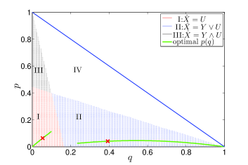
An example of the resulting decision regions derived above is presented in Fig. 1. The white region (IV) corresponds to the reconstruction decision X^=Y^π‘‹π‘Œ\hat{X}=Y. When the pair (a,b)π‘Žπ‘(a,b) is fixed, the lines that delimit the regions in the plot are given by: a​(1βˆ’p)=(1βˆ’b)​qπ‘Ž1𝑝1π‘π‘ža(1-p)=(1-b)q and (1βˆ’a)​p=b​(1βˆ’q)1π‘Žπ‘π‘1π‘ž(1-a)p=b(1-q).

Refer to caption
Figure 1: Reconstruction regions in the (p,q)π‘π‘ž(p,q) plane for a=0.1,b=0.4formulae-sequenceπ‘Ž0.1𝑏0.4a=0.1,b=0.4

III-C Deriving a tight bound on the rate distortion function

Given RW​Zβˆ—β€‹(p,q)superscriptsubscriptπ‘…π‘Šπ‘π‘π‘žR_{WZ}^{*}(p,q) as in (15) and the four expressions of the distortion function in (22), finding the bound can be formulated as a minimization problem with constraints. For every distortion level d∈[0,Dm​a​x]𝑑0subscriptπ·π‘šπ‘Žπ‘₯d\in\big{[}0,D_{max}\big{]}, the goal is to find the (p,q)π‘π‘ž(p,q) pair that minimizes the rate, while satisfying the distortion constraint:

for eachΒ d∈[0,Dm​a​x]Β minimize​RW​Zβˆ—β€‹(p,q)for eachΒ d∈[0,Dmax]Β minimizesuperscriptsubscriptπ‘…π‘Šπ‘π‘π‘ž\displaystyle\text{for each $d\in\big{[}0,D_{max}\big{]}$ minimize}\ R_{WZ}^{*}(p,q)
subject to​{0β‰€π’Ÿβ€‹(p,q)≀d≀Dm​a​xπ’Ÿβ€‹(p,q)​has a form∈{D1,D2,D3,D4}subject tocases0π’Ÿπ‘π‘žπ‘‘subscriptπ·π‘šπ‘Žπ‘₯otherwiseπ’Ÿπ‘π‘žhas a formsubscript𝐷1subscript𝐷2subscript𝐷3subscript𝐷4otherwise\displaystyle\text{subject to}\begin{cases}0\leq\mathcal{D}(p,q)\leq d\leq D_{max}\\ \mathcal{D}(p,q)\ \text{has a form}\in\{D_{1},D_{2},D_{3},D_{4}\}\end{cases} (24)

The result of the above minimization is denoted RW​Zβˆ—β€‹(d)superscriptsubscriptπ‘…π‘Šπ‘π‘‘R_{WZ}^{*}(d).

In order to establish a characterization of the bound, we need to show how a certain distortion level can be achieved, i.e., what reconstruction function should be used. For example, if the required distortion level is d=0𝑑0d=0, this can only be obtained using X^=U^π‘‹π‘ˆ\hat{X}=U, since min⁑(D2)=a/2subscript𝐷2π‘Ž2\min(D_{2})=a/2, min⁑(D3)=b/2subscript𝐷3𝑏2\min(D_{3})=b/2, and D4subscript𝐷4D_{4} is a constant.

As such, we consider all possible values for the expected distortion d𝑑d, and we must find what pairs (p,q)π‘π‘ž(p,q) can achieve it and the corresponding reconstruction strategy. As d𝑑d grows from zero to Dm​a​xsubscriptπ·π‘šπ‘Žπ‘₯D_{max}, we can derive the following conclusions:

  • β€’

    If 0≀d<a2β‹…(1βˆ’b)0π‘‘π‘Žβ‹…21𝑏0\leq d<\frac{a}{2\cdot(1-b)} we have only one reconstruction possibility, denoted R​I𝑅𝐼RI, namely X^=U,^π‘‹π‘ˆ\hat{X}=U, and d=D1𝑑subscript𝐷1d=D_{1}.

  • β€’

    If a2β‹…(1βˆ’b)≀d≀b2β‹…(1βˆ’a)π‘Žβ‹…21𝑏𝑑𝑏⋅21π‘Ž\frac{a}{2\cdot(1-b)}\leq d\leq\frac{b}{2\cdot(1-a)} we have two possible reconstructions, R​I𝑅𝐼RI and R​I​I𝑅𝐼𝐼RII (i.e. X^=U∨Y^π‘‹π‘ˆπ‘Œ\hat{X}=U\lor Y), and d𝑑d can have forms D1subscript𝐷1D_{1} or D2subscript𝐷2D_{2}.

  • β€’

    If b2β‹…(1βˆ’a)≀d≀Dm​a​x=a+b2𝑏⋅21π‘Žπ‘‘subscriptπ·π‘šπ‘Žπ‘₯π‘Žπ‘2\frac{b}{2\cdot(1-a)}\leq d\leq D_{max}=\frac{a+b}{2} we have three possible reconstructions, cases R​I𝑅𝐼RI, R​I​I𝑅𝐼𝐼RII and R​I​I​I𝑅𝐼𝐼𝐼RIII (i.e. X^=U∧Y^π‘‹π‘ˆπ‘Œ\hat{X}=U\land Y), so d𝑑d can have forms D1,D2subscript𝐷1subscript𝐷2D_{1},D_{2} or D3subscript𝐷3D_{3}.

  • β€’

    The reconstruction function X^=Y^π‘‹π‘Œ\hat{X}=Y gives constant distortion D4=Dm​a​xsubscript𝐷4subscriptπ·π‘šπ‘Žπ‘₯D_{4}=D_{max}.

Refer to caption
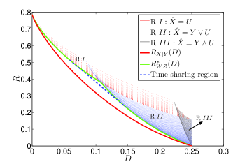
Figure 2: RX|Y​(d)subscript𝑅conditionalπ‘‹π‘Œπ‘‘R_{X|Y}(d) and Rb​o​u​n​d​(d)subscriptπ‘…π‘π‘œπ‘’π‘›π‘‘π‘‘R_{bound}(d) for a = 0.1 and b = 0.4

By numerical evaluation, the minimum for RW​Zβˆ—β€‹(d)superscriptsubscriptπ‘…π‘Šπ‘π‘‘R_{WZ}^{*}(d) can be achieved by letting X^=U^π‘‹π‘ˆ\hat{X}=U at lower distortion levels, and by letting X^=U∨Y^π‘‹π‘ˆπ‘Œ\hat{X}=U\lor Y for high distortions.

We want our bound to be a convex function; RW​Zβˆ—β€‹(d)superscriptsubscriptπ‘…π‘Šπ‘π‘‘R_{WZ}^{*}(d) on the other hand may not be convex, as it is the union of two convex curves: one corresponding to X^=U^π‘‹π‘ˆ\hat{X}=U, the other to X^=U∨Y^π‘‹π‘ˆπ‘Œ\hat{X}=U\lor Y. To this end, we must consider the lower convex envelope of the achievable points: Rb​o​u​n​d​(d)=l.c.e.​{RW​Zβˆ—β€‹(d)}subscriptπ‘…π‘π‘œπ‘’π‘›π‘‘π‘‘l.c.e.superscriptsubscriptπ‘…π‘Šπ‘π‘‘R_{bound}(d)=\text{l.c.e.}\{R_{WZ}^{*}(d)\}. This will include the common tangent of the two curves and the region is achievable through time sharing.

As an illustration, the rate distortion points in region R​i𝑅𝑖Ri of Fig. 2 correspond to the p​(q)π‘π‘žp(q) values in region i𝑖i of Fig. 1, for all i∈{I,I​I,I​I​I}𝑖𝐼𝐼𝐼𝐼𝐼𝐼i\in\{I,II,III\}. Fig. 2 also presents RW​Zβˆ—β€‹(d)superscriptsubscriptπ‘…π‘Šπ‘π‘‘R_{WZ}^{*}(d), the common tangent which completes Rb​o​u​n​d​(d)subscriptπ‘…π‘π‘œπ‘’π‘›π‘‘π‘‘R_{bound}(d), and the predictive RX|Y​(d)subscript𝑅conditionalπ‘‹π‘Œπ‘‘R_{X|Y}(d).

The solution to the minimization problem proposed has a complex form and the resulting equations cannot be solved analytically. We can therefore obtain the Rb​o​u​n​d​(d)subscriptπ‘…π‘π‘œπ‘’π‘›π‘‘π‘‘R_{bound}(d) curve only by numerically solving a logarithmic equation.

An important aspect is to answer whether the obtained rate distortion bound is tight. From [5] we know that the cardinality of the auxiliary variable Uπ‘ˆU is bounded by |𝒳|+1𝒳1|\mathcal{X}|+1, so a ternary alphabet for Uπ‘ˆU might be needed to achieve the rate distortion function. However, numerical experiments obtained with various probability input distributions Ο€πœ‹\pi, and crossover probabilities of the correlation channel (a,b)π‘Žπ‘(a,b), indicate that the proposed rate distortion bound does overlap with the rate distortion function obtained with the Blahut-Arimoto algorithm in [10]. Hence, we conjecture that a binary auxiliary variable Uπ‘ˆU is sufficient to achieve the rate distortion function and the proposed rate distortion bound Rb​o​u​n​d​(d)subscriptπ‘…π‘π‘œπ‘’π‘›π‘‘π‘‘R_{bound}(d) is tight. A thorough analysis of this aspect is left as topic of further investigation.

IV Optimal p​(U|X)𝑝conditionalπ‘ˆπ‘‹p(U|X) and rate-loss assessment

Since our bound Rb​o​u​n​d​(d)subscriptπ‘…π‘π‘œπ‘’π‘›π‘‘π‘‘R_{bound}(d) does not have an analytical form, we use a numerical approach to derive the optimal crossover values of the Xβˆ’Uπ‘‹π‘ˆX-U channel, i.e., the (p,q)π‘π‘ž(p,q) pairs, and also to find the time-sharing region.
Refer to caption
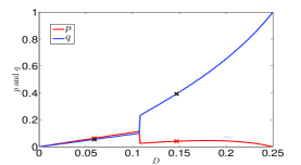
Figure 3: Optimal p​(d)𝑝𝑑p(d) and q​(d)π‘žπ‘‘q(d) for a=0.1π‘Ž0.1a=0.1 and b=0.4𝑏0.4b=0.4

The optimal crossover pairs (p,q)π‘π‘ž(p,q) that achieve the RW​Zβˆ—β€‹(d)superscriptsubscriptπ‘…π‘Šπ‘π‘‘R_{WZ}^{*}(d) bound, are plotted as p​(q)π‘π‘žp(q) in Fig. 1, while Fig. 3 presents the same (p,q)π‘π‘ž(p,q) pairs as functions of the distortion. The cross markers in both figures show the values that delimit the time sharing region. For low distortions, when the reconstruction function is X^=U^π‘‹π‘ˆ\hat{X}=U, the optimal channels are close to binary symmetric channels. When the transition to the reconstruction function X^=U∨Y^π‘‹π‘ˆπ‘Œ\hat{X}=U\lor Y occurs, there is a discontinuity in the p​(d)𝑝𝑑p(d) and q​(d)π‘žπ‘‘q(d) functions. That can be noticed in Fig. 1 as well, where the two green curve segments are disjoint.
Refer to caption
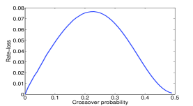
Figure 4: Rate-loss for BSC correlation with different crossover probabilities

If we fix the average distortion of the correlation channel, the highest rate-loss is in the case of the binary symmetric correlation. Fig. 4 shows the variation of the rate-loss for different crossover probabilities of the binary symmetric correlation channel Xβˆ’Yπ‘‹π‘ŒX-Y. The maximum value Δ​R=0.0765Δ𝑅0.0765\Delta R=0.0765 is obtained for the crossover a=b=0.227π‘Žπ‘0.227a=b=0.227.

V Conclusion

This paper analyzes the rate distortion problem for a binary uniform source in the presence of correlated side information, when the correlation is given by an asymmetric channel. We have derived the RX|Y​(d)subscript𝑅conditionalπ‘‹π‘Œπ‘‘R_{X|Y}(d) for the conventional predictive case, and also proposed a bound Rb​o​u​n​d​(d)subscriptπ‘…π‘π‘œπ‘’π‘›π‘‘π‘‘R_{bound}(d) for the Wyner-Ziv case. Numerical algorithms allow us to describe the optimum p​(U|X)𝑝conditionalπ‘ˆπ‘‹p(U|X) achieving the bound, as well as to establish the maximum rate-loss in the case of binary uniform sources.

References

  • [1] J.Β F. Mota, N.Β Deligiannis, and M.Β R. Rodrigues, β€œCompressed sensing with prior information: Optimal strategies, geometry, and bounds,” arXiv preprint arXiv:1408.5250, 2014.
  • [2] V.Β Toto-Zarasoa, A.Β Roumy, and C.Β Guillemot, β€œSource modeling for distributed video coding,” IEEE Trans. Circuits Syst. Video Techn., vol.Β 22, no.Β 2, pp. 174–187, Feb. 2012.
  • [3] N.Β Deligiannis, J.Β Barbarien, M.Β Jacobs, A.Β Munteanu, A.Β Skodras, and P.Β Schelkens, β€œSide-information-dependent correlation channel estimation in hash-based distributed video coding,” IEEE Trans. Image Process., vol.Β 21, no.Β 4, pp. 1934–1949, Apr. 2012.
  • [4] T.Β Berger, β€œRate-distortion theory,” Encyclopedia of Telecommunications, 1971.
  • [5] A.Β D. Wyner and J.Β Ziv, β€œThe rate-distortion function for source coding with side information at the decoder,” IEEE Trans. Inf. Theory, vol.Β 22, no.Β 1, pp. 1–10, Jan. 1976.
  • [6] Y.Β Steinberg, β€œCoding and common reconstruction,” IEEE Trans. Inf. Theory, vol.Β 55, no.Β 11, pp. 4995–5010, 2009.
  • [7] N.Β Deligiannis, A.Β Sechelea, A.Β Munteanu, and S.Β Cheng, β€œThe no-rate-loss property of wyner-ziv coding in the z-channel correlation case,” IEEE Comm. Lett., vol.Β 18, no.Β 10, pp. 1675–1678, 2014.
  • [8] R.Β Zamir, β€œThe rate loss in the wyner-ziv problem,” IEEE Trans. Inf. Theory, vol.Β 42, no.Β 6, pp. 2073–2084, 1996.
  • [9] R.Β E. Blahut, β€œComputation of channel capacity and rate-distortion functions,” Information Theory, IEEE Transactions on, vol.Β 18, no.Β 4, pp. 460–473, 1972.
  • [10] S.Β Cheng, V.Β Stankovic, and Z.Β Xiong, β€œComputing the channel capacity and rate-distortion function with two-sided state information,” IEEE Trans. Inf. Theory, vol.Β 51, no.Β 12, pp. 4418–4425, 2005.