$B\rightarrow\pi\ell\nu$ at zero recoil from lattice QCD with physical $u/d$ quarks

Abstract

The exclusive semileptonic decay $B\rightarrow\pi\ell\nu$ is a key process for the determination of the Cabibbo-Kobayashi-Maskawa matrix element $V_{ub}$ from the comparison of experimental rates as a function of $q^{2}$ with theoretically determined form factors. The sensitivity of the form factors to the $u/d$ quark mass has meant significant systematic uncertainties in lattice QCD calculations at unphysically heavy pion masses. Here we give the first lattice QCD calculations of this process for u/d quark masses going down to their physical values, calculating the $f_{0}$ form factor at zero recoil to 3%. We are able to resolve a long-standing controversy by showing that the soft-pion theorem result $f_{0}(q^{2}_{max})=f_{B}/f_{\pi}$ does hold as $m_{\pi}\rightarrow 0$. We use the Highly Improved Staggered Quark formalism for the light quarks and show that staggered chiral perturbation theory for the $m_{\pi}$ dependence is almost identical to continuum chiral perturbation theory for $f_{0}$, $f_{B}$ and $f_{\pi}$. We also give results for other processes such as $B_{s}\rightarrow K\ell\nu$.

I Introduction

The exclusive semileptonic process, $B\rightarrow\pi\ell\nu$, is a key one for flavour physics because it gives access to the Cabibbo-Kobayashi-Maskawa matrix element $V_{ub}$ from a process involving two ‘gold-plated’ (stable in QCD) mesons, $B$ and $\pi$. $V_{ub}$ is determined by comparing the experimental rate for the process to that determined from theoretical calculations of hadronic parameters known as form factors which are functions of the squared 4-momentum transfer, $q^{2}$, between the $B$ and the $\pi$. The form factors encapsulate the information about how likely it is for a $\pi$ meson with a specific momentum to form when a $b$ quark inside a $B$ meson changes into a $u$ quark with emission of a $W$ boson. If the calculations of the form factors are done in lattice QCD then the full effect of QCD interactions that keep the quarks bound inside the mesons is taken into account.

Lattice QCD calculations for this process are particularly difficult, however, because the results are sensitive to the mass of the $u/d$ quarks that form the $\pi$ meson. Existing lattice QCD calculations have used $u/d$ quarks that have heavier masses than in the real world and results then have to be extrapolated to the physical point. The value of the $u/d$ quark masses, and hence the $\pi$ mass, also affects the $q^{2}$ value for a given $\pi$ spatial momentum and, since the form factors are strongly varying functions of $q^{2}$, this gives further dependence on the quark masses. For recent lattice QCD results for $B\rightarrow\pi\ell\nu$ form factors see Bailey et al. (2015); Flynn et al. (2015).

Lattice QCD calculations for the form factors are most reliable close to the ‘zero recoil’ point where the $\pi$ has small spatial momentum (and hence relatively small discretisation errors). This corresponds to being close to the maximum value of $q^{2}$, $(m_{B}-m_{\pi})^{2}$. In this regime it is possible to use soft pion relations coupled to Heavy Quark Effective Theory to derive expectations for the functional dependence of form factors on the heavy quark mass, $m_{b}$, and on the $\pi$ meson mass. Since these relationships come from a well understood theoretical framework it is important to test them against lattice QCD results.

It was apparent in quenched lattice QCD calculations many years ago that there were large deviations between lattice results and the expected dependence on $m_{b}$ and $m_{\pi}$; see Onogi (1998); Hashimoto (2000) for a review. Relatively heavy $u/d$ quark masses were used in these early calculations, often close to the $s$ quark mass.

Here we revisit this issue with results from lattice QCD that include the full effect of sea quarks ($u$, $d$, $s$ and $c$) but, more importantly, include $u$ and $d$ quarks with masses at their very small physical values for the first time. We focus on the soft pion relation which gives the scalar form factor $f_{0}$ at the zero recoil point in terms of the ratio of $B$ and $\pi$ decay constants as $m_{\pi}\rightarrow 0$ Dominguez et al. (1990); Wise (1992); Burdman and Donoghue (1992); Wolfenstein (1992):

$$f_{0}(q^{2}_{max})=\frac{f_{B}}{f_{\pi}}.$$ (1)

This relationship has been shown to hold through $\mathcal{O}(\Lambda/m_{h})$ in an expansion in powers of the inverse heavy quark mass, $m_{h}$ Burdman et al. (1994), and we therefore expect it to work at the 1% level for $b$ quarks. A test of this in lattice QCD calculations can then provide important confirmation of how well we understand the $u/d$ quark mass dependence for a process $B\rightarrow\pi\ell\nu$ for which this is critical.

Here we show that indeed the soft-pion relation does emerge from lattice QCD calculations as $m_{\pi}\rightarrow 0$ for a fixed heavy quark mass tuned to that of the $b$. This calculation builds on the very accurate results for $f_{B}$ and $f_{\pi}$ that we have been able to obtain at physical $u/d$ quark masses Dowdall et al. (2013a, b) and benefits from the fact that the renormalisation factors of the temporal vector and temporal axial-vector heavy-light currents are the same for our light quark formalism and so renormalisation uncertainties are minimised.

In addition we give a precise result for $f_{0}(q^{2}_{max})$ for physical $u/d$ quark masses (where corrections to the soft-pion relation are substantial). This is a useful comparison point for lattice QCD calculations that are done with unphysical $u/d$ quark masses, as a test of extrapolations in the $u/d$ quark mass. Although $f_{0}$ itself is not accessible in experiment, lattice QCD calculations of it should agree, and it is important to test this using different discretisations of QCD. $f_{0}(q^{2}_{max})$ is the most accurately determined form factor for a lattice QCD calculation of $B\rightarrow\pi$ decay and so a good number for calibration.

For comparison we also give results for $f_{0}(q^{2}_{max})$ for $B_{s}\rightarrow K\ell\nu$ decay, which is another physical process, and for $B_{s}\rightarrow\eta_{s}\ell\nu$, which does not occur in the real world. The latter decay is again useful for comparison between lattice QCD calculations.

The paper is laid out as follows: In Section II we describe the lattice calculation of the correlation functions needed to extract the scalar form factor and its ratio to $f_{B}/f_{\pi}$. We use the Highly Improved Staggered Quark (HISQ) action for the light quarks and improved NonRelativistic QCD (NRQCD) for the $b$ quark. In Section III we give the results and determine the ratio both at the physical $m_{\pi}$ and as $m_{\pi}\rightarrow 0$. Section IV includes a comparison of our values with those from lattice QCD calculations that extrapolated results from heavier than physical values of $m_{\pi}$ and Section V provides our conclusions. In Appendix A we discuss the staggered quark chiral perturbation theory that we use for $f_{B}$, $f_{\pi}$ and $f_{0}$ and show that it is in fact very continuum-like in its approach to $m_{\pi}=0$.

II Lattice calculation

We use ensembles of lattice gluon configurations provided by the MILC collaboration Bazavov et al. (2013) at three values of the lattice spacing, $a\approx$ 0.15 fm, 0.12 fm and 0.09 fm. The configurations include the effect of $u$, $d$, $s$ and $c$ quarks in the sea using the HISQ formalism Follana et al. (2007) and a gluon action improved through $\mathcal{O}(\alpha_{s}a^{2})$ Hart et al. (2009). These then give significant improvements in the control of systematic errors from finite lattice spacing and light quark mass effects over earlier configurations.

Set	$a$/fm	$am_{l}$	$am_{s}$	$am_{c}$	$L_{s}/a$	$L_{t}/a$	$N_{\mathrm{cfg}}$
1	0.1474(5)(14)	0.013	0.065	0.838	16	48	1020
2	0.1463(3)(14)	0.0064	0.064	0.828	24	48	1000
3	0.1450(3)(14)	0.00235	0.0647	0.831	32	48	1000
4	0.1219(2)(9)	0.0102	0.0509	0.635	24	64	1052
5	0.1195(3)(9)	0.00507	0.0507	0.628	32	64	1000
6	0.1189(2)(9)	0.00184	0.0507	0.628	48	64	1000
7	0.0884(3)(5)	0.0074	0.037	0.440	32	96	1008
8	0.0873(2)(5)	0.0012	0.0363	0.432	64	96	620

Table 1: Details of gluon field configurations used in this calculation Bazavov et al. (2013). $a$ is the lattice spacing, fixed from the mass difference between the $\Upsilon^{\prime}$ and $\Upsilon$ in Dowdall et al. (2012a). The first error is from statistics and the second from NRQCD systematics in that determination and from experiment. Sets 1, 2 and 3 are ‘very coarse’, sets 4, 5 and 6 are ‘coarse’ and sets 7 and 8 are ‘fine’. $am_{l}$, $am_{s}$ and $am_{c}$ are the light ($u$ and $d$ are taken to have the same mass), strange and charm sea quark masses. Sets 3, 6 and 8 have $m_{l}$ at close to its physical value. $L_{s}/a$ and $L_{t}/a$ are the number of lattice sites in the spatial and temporal directions respectively and $N_{cfg}$ is the number of configurations in the ensemble. We calculate propagators from 16 time sources on each ensemble (4 on set 8) to increase statistics.

We work at three different values of the $u/d$ quark masses (which are taken to be degenerate and will be referred to as light ($l$) quarks) in the sea. These correspond to approximately one-fifth and one-tenth of the $s$ quark mass and the physical average $u/d$ quark mass ($m_{s}/27.5$ Olive et al. (2014)). The lattice spacing on these configurations is determined for this calculation from the mass difference between the $\Upsilon^{\prime}$ and the $\Upsilon$ Dowdall et al. (2012a). Table 1 lists the parameters of the ensembles.

On these configurations we calculate $l$ and $s$ quark propagators using the HISQ action. The $l$ quarks are taken to have the same mass as is used in the sea. For the $s$ quarks we retune the valence mass to be closer to the physical $s$ quark mass and so it is slightly different from that in the sea Dowdall et al. (2012a). Values are given in Table 2. We also calculate $b$ quark propagators using the improved NRQCD Lepage et al. (1992) action developed in Dowdall et al. (2012a); Hammant et al. (2013).

Set	$am_{s}^{\rm val}$	$am_{b}$	$u_{0L}$	$c_{1},c_{6}$	$c_{5}$	$c_{4}$
1	0.0641	3.297	0.8195	1.36	1.21	1.22
2	0.0636	3.263	0.82015	1.36	1.21	1.22
3	0.0628	3.25	0.8195	1.36	1.21	1.22
4	0.0522	2.66	0.8340	1.31	1.16	1.20
5	0.0505	2.62	0.8349	1.31	1.16	1.20
6	0.0507	2.62	0.8341	1.31	1.16	1.20
7	0.0364	1.91	0.8525	1.21	1.12	1.16
8	0.0360	1.89	0.8518	1.21	1.12	1.16

Table 2: Summary of the valence $s$ quark mass and valence $b$ quark mass and other action parameters for the NRQCD action on the different ensembles of Table 1. The $s$ and $b$ quark masses in lattice units (columns 2 and 3) were tuned in Dowdall et al. (2012a); Colquhoun et al. (2015a). Column 4 gives the parameter $u_{0L}$ used for ‘tadpole-improving’ the gluon field Dowdall et al. (2012a, 2013a) and columns 5, 6 and 7 give the coefficients of kinetic and chromomagnetic terms used in the NRQCD action. $c_{1}$ ($c_{6}$ has the same value), $c_{5}$ and $c_{4}$ are correct through $\mathcal{O}(\alpha_{s})$ Dowdall et al. (2012a); Hammant et al. (2013).

The NRQCD Hamiltonian we use is given by Lepage et al. (1992):

$$e^{-aH} = \left(1-\frac{a\delta H}{2}\right)\left(1-\frac{aH_{0}}{2n_{h}}\right)^{n_{h}}U_{t}^{{\dagger}}$$ (2)

$$\times\left(1-\frac{aH_{0}}{2n_{h}}\right)^{n_{h}}\left(1-\frac{a\delta H}{2}\right)$$

with

$$aH_{0} = -\frac{\Delta^{(2)}}{2am_{b}},$$

$$a\delta H = -c_{1}\frac{(\Delta^{(2)})^{2}}{8(am_{b})^{3}}+c_{2}\frac{i}{8(am_{b})^{2}}\left(\bf{\nabla}\cdot\tilde{\bf{E}}\right.-\left.\tilde{\bf{E}}\cdot\bf{\nabla}\right)$$ (3)

$$-c_{3}\frac{1}{8(am_{b})^{2}}\bf{\sigma}\cdot\left(\tilde{\bf{\nabla}}\times\tilde{\bf{E}}\right.-\left.\tilde{\bf{E}}\times\tilde{\bf{\nabla}}\right)$$

$$-c_{4}\frac{1}{2am_{b}}\,{\bf{\sigma}}\cdot\tilde{\bf{B}}+c_{5}\frac{\Delta^{(4)}}{24am_{b}}$$

$$-c_{6}\frac{(\Delta^{(2)})^{2}}{16n_{h}(am_{b})^{2}}.$$

Here $\nabla$ is the symmetric lattice derivative and $\Delta^{(2)}$ and $\Delta^{(4)}$ the lattice discretization of the continuum $\sum_{i}D_{i}^{2}$ and $\sum_{i}D_{i}^{4}$ respectively. $am_{b}$ is the bare $b$ quark mass in units of the lattice spacing. $n_{h}$ is a stability parameter set equal to 4 here. The gluon field is tadpole-improved, which means dividing all the links, $U_{\mu}(x)$ by a tadpole-parameter, $u_{0}$, before constructing covariant derivatives or chromo-electric or magnetic fields. For $u_{0}$ we took the mean trace of the gluon field in Landau gauge, $u_{0L}$ Dowdall et al. (2012a). $\bf\tilde{E}$ and $\bf\tilde{B}$ are the chromoelectric and chromomagnetic fields calculated from an improved clover term Gray et al. (2005). They are made anti-hermitian but not explicitly traceless, to match the perturbative calculations done using this action.

Given the NRQCD action above, the heavy quark propagator is readily calculated from a simple lattice time evolution equation Lepage et al. (1992) which is numerically very fast. The heavy quark propagator is given by:

$$G_{b}({\bf x},t+1)=e^{-aH}G_{b}({\bf x},t)$$ (4)

with starting condition:

$$G_{b}({\bf x},0)=\phi({\bf x})\Gamma({\bf x}).$$ (5)

Here $\Gamma$ is a matrix in (2-component) spin space and $\phi({\bf x})$ is a function of spatial position, to be discussed below. We can use such a function because we fix the gluon field configurations to Coulomb gauge.

The terms in $\delta H$ in eq. (3) have coefficients $c_{i}$ whose values can be fixed from matching lattice NRQCD to full QCD perturbatively, giving the $c_{i}$ the expansion $1+c^{(1)}_{i}\alpha_{s}+\mathcal{O}(\alpha_{s}^{2})$. Here we include $\mathcal{O}(\alpha_{s})$ corrections to the coefficients of the sub-leading kinetic terms, $c_{1}$, $c_{5}$ and $c_{6}$, and the chromomagnetic term, $c_{4}$ Dowdall et al. (2012a); Hammant et al. (2013). The $b$ quark mass parameter, $am_{b}$, is nonperturbatively tuned to the correct value by calculating the spin-average of the ‘kinetic masses’ of the $\Upsilon$ and $\eta_{b}$ as described in Dowdall et al. (2012a). We are able to do this to 1%, limited by the accuracy of the determination of the lattice spacing to convert the kinetic mass to physical units. The values used for $am_{b}$, $u_{0L}$ and $c_{i}$ on the different ensembles are given in Table 2.

We use the same NRQCD action for both heavyonium and for heavy-light meson calculations since it is accurate for both. For heavy-light calculations, which concern us here, the power counting in the heavy-quark velocity is equivalent to power-counting in inverse powers of the heavy quark mass. The NRQCD action above is then fully improved through $\mathcal{O}(\alpha_{s}\Lambda/m_{b})$. It has already been used for accurate calculations of the $\Upsilon$ spectrum and properties Dowdall et al. (2012a); Daldrop et al. (2012); Dowdall et al. (2014); Colquhoun et al. (2015a) and $B$, $B_{s}$ and $B_{c}$ meson masses Dowdall et al. (2012b) and decay constants Dowdall et al. (2013a); Colquhoun et al. (2015b), including those of their vector partners.

Set	$a_{sm}$	$T$
1,2	2.0,4.0	10,13,16
3	2.0,4.0	9,12,15
4	2.5,5.0	14,19,24
5,6	2.0,4.0	14,19,24
7	3.425,6.85	19,24,29
8	3.425,6.85	20,27,34

Table 3: Summary of the smearing radii of the smearing functions used for the $b$ quark propagators on the different sets of configurations in Table 1. Column 3 gives the different $T$ values used for the creation time-slice for the $B$ meson.

For the calculation of the $B\rightarrow\pi\ell\nu$ form factor we need (Goldstone) $\pi$ meson correlation functions, $B$ meson correlation functions and ‘3-point’ correlation functions that connect the $B$ meson to the $\pi$. Here we work with $B$ and $\pi$ mesons at rest. The $\pi$ meson correlators were calculated in Dowdall et al. (2013b) and are simply given by:

$$C_{\pi}(t)=\frac{1}{4}\left<\sum_{\vec{x}}\mathrm{tr}\left|g(\vec{x},t)\right|^{2}\right>$$ (6)

where $g(\vec{x},t)$ is a staggered quark propagator with source at $t=0$, $\mathrm{tr}$ denotes a trace over color indices and the angle brackets denote an average over gluon field configurations in the ensemble. We use random wall sources to improve statistical errors. The factor of 1/4 is needed to account for the number of staggered quark ‘tastes’ because the correlator is a staggered quark loop. Fitting these ‘2-point’ correlators to the standard multi-exponential form

$$C_{\pi}(t)=\sum_{k=0}^{n_{exp}-1}a_{\pi,k}^{2}\left(e^{-E_{\pi,k}t}+e^{-E_{\pi,k}(T-t)}\right)$$ (7)

allows the extraction of the ground-state $\pi$ mass ($\equiv E_{\pi,0}$). The amplitude $a_{\pi,0}$ gives $\langle 0|P|\pi\rangle/(\sqrt{2m_{\pi}})$ where $P$ is the pseudoscalar density. Using the PCAC relation we can convert this to $f_{\pi}$:

$$f_{\pi}=2m_{l}a_{\pi,0}\sqrt{(2/E_{\pi,0}^{3})}$$ (8)

and note that $f_{\pi}$ is absolutely normalised here. Results for $m_{\pi}$ and $f_{\pi}$ are given in Dowdall et al. (2013b). Statistical errors below 0.1% are obtained.

Staggered quarks have numerical efficiency advantages as a result of having no spin degree of freedom. A 4-component naive quark propagator, $\tilde{g}$, can be simply obtained from a staggered quark propagator, $g$, from point $x$ to point $y$ by reversing the staggering transformation:

$$\tilde{g}(x,y) = g(x,y)\Omega(x)\Omega^{{\dagger}}(y)$$ (9)

$$\Omega(x) = \prod_{\mu=1}^{4}(\gamma_{\mu})^{x_{\mu}}.$$

We can then use $\tilde{g}$ straightforwardly in combination with other propagators that carry a spin component Wingate et al. (2003), for example an NRQCD $b$ quark propagator. $B$ meson correlators at zero spatial momentum were made in this way in Dowdall et al. (2013a). NRQCD $b$ quark and staggered light quark propagators are simply combined to make a pseudoscalar meson (with operator $\overline{\Psi}_{b}(x)\gamma_{5}\Psi_{l}(x)$) as:

$$C_{B}(t)=\left<\sum_{\vec{x}}\mathrm{tr}[\mathrm{Tr}\Omega^{{\dagger}}(x)G_{b}(\vec{x},t)]g^{{\dagger}}(\vec{x},t)\right>.$$ (10)

Here $\mathrm{Tr}$ is a spin trace. In this equation both $G_{b}$ and $g$ are calculated from a simple delta function source at the origin (and $\Omega(0)=1$).

To improve our statistical precision we use a random wall source for both propagators which adds the technical complication that $\Omega^{{\dagger}}(\vec{x},t=0)$ must be used, along with the U(1) random noise field, as the source for the NRQCD propagator Gregory et al. (2011). In addition we use 3 different smearing functions for the source of the $b$ quark in eq. (5): a delta function and two exponentials with different radii, $a_{sm}$, given in Table 3. Thus, in eq. (5), $\Gamma=\Omega(\vec{x},t=0)$ and, for the smeared case,

$$\phi(\vec{x})=\sum_{\vec{y}}e^{(-|\vec{x}-\vec{y}|/a_{sm})}\eta(\vec{y})$$ (11)

with $\eta(\vec{y})$ a random field from U(1), and a 3-vector in colour space. For the staggered quark propagator the source is simply $\eta(\vec{x})$.

We obtain a $3\times 3$ matrix of correlation functions from the use of the 3 different smearings for the $b$ quark at source and sink. This can be fit to a multi-exponential form as for the $\pi$ meson, except that the correlator has a simple exponential form in time rather than a cosh because NRQCD $b$ quarks propagate in one direction in time only. To improve statistics we average over forward-in-time and backward-in-time directions. The fit enables us to extract $B$ meson energies (these are not equal to the meson masses because of the NRQCD energy offset) and amplitudes that depend on the smearing function used Dowdall et al. (2012b). We use a fit function

$$C_{B}(t) = \sum_{m=0}^{m_{exp}-1}c(\phi_{sc},m)c^{*}(\phi_{sk},m)e^{-E_{m}t}$$

$$- (-1)^{t}\sum_{m^{\prime}=1}^{m_{exp}-1}d(\phi_{sc},m^{\prime})d^{*}(\phi_{sk},m^{\prime})e^{-E^{\prime}_{m^{\prime}}t},$$

where $sc$ and $sk$ denote source and sink respectively. The second line captures the presence of ‘oscillating’ opposite parity states in the correlator that are a result of using a staggered light quark. Having multiple smearing functions improves the fit significantly because they enhance the signal for the ground-state at small $t$ values which counteracts the relatively poor signal-noise in $B$ correlators at large $t$.

The decay constant for the $B$ meson is defined from the matrix element of the continuum temporal axial current between the vacuum and a $B$ meson at rest:

$$f_{B}m_{B}=\langle 0|A_{0}|B(\vec{p}=0)\rangle.$$ (13)

To determine this accurately in our lattice QCD calculations requires finding a good approximation to the continuum $A_{0}$ current in terms of bilinears made of HISQ light and NRQCD $b$ quarks.

The most accurate calculation to date is in Dowdall et al. (2013a) where we use a matching through $\alpha_{s}\Lambda/m_{b}$, consistent with the level of accuracy in our improved NRQCD action:

$$A_{0}=(1+z_{0}\alpha_{s})\left[J_{A_{0}}^{(0)}+(1+z_{1}\alpha_{s})J_{A_{0}}^{(1)}+z_{2}\alpha_{s}J_{A_{0}}^{(2)}\right]$$ (14)

with

$$J_{A_{0}}^{(0)} = \bar{\Psi}_{l}\gamma_{5}\gamma_{0}\Psi_{b}$$ (15)

$$J_{A_{0}}^{(1)} = \frac{-1}{2m_{b}}\bar{\Psi}_{l}\gamma_{5}\gamma_{0}\gamma\cdot\nabla\Psi_{b}$$

$$J_{A_{0}}^{(2)} = \frac{-1}{2m_{b}}\bar{\Psi}_{l}\gamma\cdot\overleftarrow{\nabla}\gamma_{0}\gamma_{5}\gamma_{0}\Psi_{b}.$$

The $\mathcal{O}(\alpha_{s})$ matching coefficients $z_{0}$, $z_{1}$ and $z_{2}$ are given in Table 4. In Dowdall et al. (2013a) we used $\alpha_{s}\equiv\alpha_{V}(n_{f}=4,2/a)$ to evaluate the matching coefficients above. We do that again here and also give in Table 4 the value of $\alpha_{s}$ on each ensemble. These are obtained by converting and running down the result $\alpha_{\overline{MS}}(n_{f}=5,M_{Z})=0.1185(6)$ Olive et al. (2014); McNeile et al. (2010).

Table 4: Coefficients for the perturbative matching of the temporal axial vector and temporal vector currents (eq. (14)) from Dowdall et al. (2013a). $z_{0}=\rho_{0}-\zeta_{10}$, $z_{1}=\rho_{1}-z_{0}$, $z_{2}=\rho_{2}$ from Monahan et al. (2013). Column 5 gives the values of $\alpha_{s}$ used in the matching. This is determined in V-scheme with 4 sea quarks at scale $2/a$.

Set	$z_{0}$	$z_{1}$	$z_{2}$	$\alpha_{V}(2/a)$
1	0.024(2)	0.024(3)	-1.108(4)	0.346
2	0.022(2)	0.024(3)	-1.083(4)	0.345
3	0.022(1)	0.024(2)	-1.074(4)	0.343
4	0.006(2)	0.007(3)	-0.698(4)	0.311
5	0.001(2)	0.007(3)	-0.690(4)	0.308
6	0.001(2)	0.007(2)	-0.690(4)	0.307
7	-0.007(2)	-0.031(4)	-0.325(4)	0.267
8	-0.007(2)	-0.031(4)	-0.318(4)	0.266

To determine the matrix element of $A_{0}$ and hence $f_{B}$ we calculate the matrix elements of each of the $J_{A_{0}}^{(i)}$ by implementing that operator at the sink of the $B$ meson correlation function. For $J_{A_{0}}^{(0)}$ this is simply the local operator used in eq. (10) (since the $\gamma_{0}$ has no effect on a 2-component NRQCD $b$ quark) and $J_{A_{0}}^{(1)}$ and $J_{A_{0}}^{(2)}$ are implemented by differentiating the appropriate propagator before combining into a meson correlator. For a $B$ meson at rest the matrix elements of $J_{A_{0}}^{(1)}$ and $J_{A_{0}}^{(2)}$ are equal since the momenta of the $b$ and $l$ quarks are equal and opposite.

From simultaneous fits, using eq. (II), to the $3\times 3$ matrix of $B$ meson correlators described above, along with correlators that have $J_{A_{0}}^{(1)}$ inserted at the sink, the amplitude $c(A_{0},0)$ that corresponds to the annihilation of the ground-state $B$ meson with the $A_{0}$ current can be determined. The amplitude is given by

$$c(A_{0},0)=\frac{\langle 0|A_{0}|B\rangle}{\sqrt{2m_{B}}}=\frac{f_{B}\sqrt{m_{B}}}{\sqrt{2}}.$$ (16)

Results for $\Phi=f_{B}\sqrt{m_{B}}$ for $B$ and $B_{s}$ are given on the sets of gluon field ensembles used here in Dowdall et al. (2013a) and we use the same $B$ meson correlation functions here.

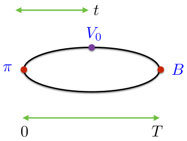
Figure 1: A schematic diagram of the 3-point correlator needed for $B\rightarrow\pi\ell\nu$ decay at zero recoil.

The new correlation functions that we have calculated here are the ‘3-point’ functions for $B\rightarrow\pi\ell\nu$ decay, illustrated in Fig. 1. For these a light quark propagator from a random wall source at $t=0$ is used, at time-slice $T$ and convoluted with each of the $b$-quark smearing functions, as the source of a NRQCD $b$ propagator. This propagates backwards in time to time-slice $t$ where it is connected via a temporal vector current to another identical light quark propagator, joined to the first one at the source time-slice in the appropriate way to form a $\pi$ meson. For this to work with staggered light quark propagators $\Omega$ matrices must be inserted at $T$ and $t$ to reinstate the light quark spin. Both the $B$ meson and $\pi$ meson are at rest. We use multiple $T$ values so that we can fit the 3-point function both as a function of $t$ and as a function of $T$. The $T$ values used on each ensemble are given in Table 3.

Because of the chiral symmetry of staggered quarks the matching of the NRQCD-HISQ temporal vector current to continuum QCD takes the same form as the temporal axial vector current:

$$V_{0}=(1+z_{0}\alpha_{s})\left[J_{V_{0}}^{(0)}+(1+z_{1}\alpha_{s})J_{V_{0}}^{(1)}+z_{2}\alpha_{s}J_{V_{0}}^{(2)}\right]$$ (17)

with

$$J_{V_{0}}^{(0)} = \bar{\Psi}_{l}\gamma_{0}\Psi_{b}$$ (18)

$$J_{V_{0}}^{(1)} = \frac{-1}{2m_{b}}\bar{\Psi}_{l}\gamma_{0}\gamma\cdot\nabla\Psi_{b}$$

$$J_{V_{0}}^{(2)} = \frac{-1}{2m_{b}}\bar{\Psi}_{l}\gamma\cdot\overleftarrow{\nabla}\Psi_{b}.$$

We calculate the 3-point function inserting each of the $J_{V_{0}}^{(i)}$ at the heavy-light vertex at $t$. We can then fit the 3-point functions along with 2-point correlators discussed above to determine the matrix element of $V_{0}$ between $\pi$ and $B$. For $B$ and $\pi$ at rest the matrix elements of $J_{V_{0}}^{(1)}$ and $J_{V_{0}}^{(2)}$ are equal and so we only calculate one of them.

The 3-point correlation function is fit to the form:

$$C_{3pt}(t,T)=$$

$$\sum_{j,k=0}^{n_{exp}-1}a_{\pi,j}V_{nn}(j,k)c^{*}_{B,k}fn_{\pi}(E_{\pi,j},t)fn_{B}(E_{B,k},T-t)$$

$$- \sum_{j,k^{\prime}=0}^{n_{exp}-1}a_{\pi,j}V_{no}(j,k^{\prime})d^{*}_{B,k^{\prime}}fn_{\pi}(E_{\pi,j},t)fo_{B}(E^{\prime}_{B,k^{\prime}},T-t)$$

where $n$ denotes normal parity states and again oscillating terms appear for the $B$ meson from higher mass opposite-parity ($o$) states. Here

$$fn_{\pi}(E,t) = e^{-Et}+e^{-E(T-t)},$$ (20)

$$fn_{B}(E,t) = e^{-Et},$$

$$fo_{B}(E,t) = (-1)^{t}fn_{B}(E,t).$$

The amplitudes $a_{\pi,k}$ and energies $E_{\pi,k}$ are the same amplitudes and energies as in the $\pi$ 2-point fits (eq. (7)). The amplitudes $c^{*}_{B,k}$ and $d^{*}_{B,k^{\prime}}$ and energies $E_{B,k}$ and $E^{\prime}_{B,k^{\prime}}$ are the same as in the $B$ 2-point fit (eq. (II)) for the corresponding smearing function for the $B$ meson.

The fit parameter $V_{nn}(0,0)$ is the result that we need for the ground-state $B$ to ground-state $\pi$ matrix element for a current, $J$, inserted at $t$. Using the standard relativistic normalisation of states:

$$V^{J}_{nn}(0,0)=\frac{\langle\pi|J|B\rangle}{2\sqrt{m_{\pi}m_{B}}}.$$ (21)

Combining results from $J_{V_{0}}^{(0)}$, $J_{V_{0}}^{(1)}$ and $J_{V_{0}}^{(2)}$ as in eq. (17) gives an amplitude corresponding to the continuum QCD current, $V_{0}$, which we denote as $V^{V_{0}}$. This is directly related to the matrix element of $V_{0}$ between $\pi$ and $B$ as in eq. (21). Since, at zero recoil

$$\langle\pi|V_{0}|B\rangle=f_{0}(q^{2}_{max})(m_{B}+m_{\pi})$$ (22)

then

$$2\sqrt{m_{\pi}}V^{V_{0}}=f_{0}(q^{2}_{max})\sqrt{m_{B}}\left(1+\frac{m_{\pi}}{m_{B}}\right).$$ (23)

We can therefore directly extract $f_{0}(q^{2}_{max})\sqrt{m_{B}}(1+m_{\pi}/m_{B})$ from our fit results. Dividing by $\sqrt{2}$ times the amplitude from eq. (16) gives $f_{0}(q^{2}_{max})(1+m_{\pi}/m_{B})/f_{B}$. Note that in forming this ratio the overall renormalisation factor of the temporal axial/vector current cancels (eqs. (14) and (17)). Hence this ratio has significantly lower systematic errors from renormalisation/matching than the individual quantities $f_{0}$ and $f_{B}$. The division can be done inside the fit code and therefore correlations between the fit parameters can be taken into account to reduce statistical errors. Because of the inclusion of relativistic/radiative corrections to the currents, the ratio is accurate through $\alpha_{s}\Lambda/m_{b}$ in a power-counting in inverse powers of the $b$ quark mass. Multiplication by the amplitude and energy combination that gives $f_{\pi}$ is also readily done inside the fit to give a result for

$$R_{B\pi}=\frac{f_{0}(q^{2}_{max})(1+m_{\pi}/m_{B})}{[f_{B}/f_{\pi}]}.$$ (24)

This is the quantity that we will work with, examining its limit as $m_{\pi}\rightarrow 0$ where the factor of $(1+m_{\pi}/m_{B})$ vanishes and we expect the answer 1 from the soft-pion relation, eq. (1). From this we can also obtain the ratio at the physical value of $m_{\pi}$ and thereby the value of $f_{0}(q^{2}_{max})$ at that point.

We have also calculated the appropriate 3-point correlation functions for the processes $B_{s}\rightarrow K\ell\nu$ and $B_{s}\rightarrow\eta_{s}\ell\nu$ and combined these with the appropriate 2-point functions from Dowdall et al. (2013a, b) to obtain an analogous ratio for $f_{0}(q^{2}_{max})$ to that above ($R_{B_{s}K}$ and $R_{B_{s}\eta_{s}}$ respectively). In these cases we can also extract a result for $f_{0}(q^{2}_{max})$ for physical quark masses that is accurate through $\alpha_{s}\Lambda/m_{b}$.

III Results

III.1 $B\rightarrow\pi$

As discussed in Section II, we fit our results for 3-point functions for $B\rightarrow\pi$ and 2-point functions for $B$ and $\pi$ simultaneously to the forms given in eqs. (7), (II) and (II). We use a constrained fitting technique Lepage et al. (2002) so that we can include uncertainties in our fitted results for the ground-state coming from the presence of excited states in the correlation function. The prior value taken on the difference in mass between adjacent states (both in normal and oscillating channels) is 600(300) MeV and (for the $B$) on the difference between the ground-state and the first oscillating state is 400(200) MeV. The prior taken on all 2-point amplitudes is 0.0(1.0) and for 3-point amplitudes 0.0(5.0). For our normalisation of the raw correlators these widths correspond to 3–5 times the ground-state value and so provide a loose constraint.

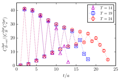
Figure 2: The ratio of the 3-point correlator for $B\rightarrow\pi$ decay to the product of 2-point correlators for $B$ and $\pi$ as a function of lattice time. The $B$ is at $t=0$ and the $\pi$ at $T$ here, since this illustrates more clearly the convergence of results for different $T$. Results are for coarse set 4, statistical errors only.

Figure 2 illustrates the quality of our results by showing a plot of the ratio of 3-point to 2-point correlators for $B\rightarrow\pi$ decay on coarse set 4. Statistical errors are small and, although oscillating terms are strong on the $B$ side of the 3-point correlator, it is clear that results at different $T$ values are consistent so that we are able to isolate ground-state amplitudes.

Set	$V^{(0)}_{nn}(0,0)$	$V^{(1)}_{nn}(0,0)$	$V^{V_{0}}$	$g^{B\pi}_{0}(q^{2}_{\mathrm{m}ax})$
1	2.072(33)	-0.115(8)	2.017(33)	1.961(32)
2	2.581(40)	-0.159(5)	2.499(40)	2.037(33)
3	3.637(49)	-0.247(21)	3.505(61)	2.236(39)
4	2.110(32)	-0.129(3)	2.012(31)	1.761(27)
5	2.675(27)	-0.182(3)	2.532(27)	1.855(20)
6	3.837(50)	-0.289(5)	3.609(50)	2.061(28)
7	2.154(17)	-0.156(2)	2.010(17)	1.508(13)
8	3.829(91)	-0.334(10)	3.520(85)	1.683(41)

Table 5: Columns 2 and 3 give ground-state parameters $V_{nn}(0,0)$ (in lattice units) from our combined 2-point and 3-point fit for $B\rightarrow\pi$ decay. $V^{(0)}_{nn}$ corresponds to current $J_{V_{0}}^{(0)}$ and $V^{(1)}_{nn}$ to $J_{V_{0}}^{(1)}$ (see eq. (18)). $J_{V_{0}}^{(2)}$ has equal amplitude to $J_{V_{0}}^{(1)}$ at zero recoil and so is not given separately. In column 4 results are combined as in eq. (17) into an equivalent parameter for the full QCD current, $V_{0}$. Column 5 presents the results as the combination $g^{B\pi}_{0}\equiv f_{0}\sqrt{am_{B}}(1+m_{\pi}/m_{B})$ in lattice units.

Set $\frac{f^{(0)}_{0}(q^{2}_{\mathrm{max}})(1+m_{\pi}/m_{B})}{(f^{(0)}_{B}/f_{\pi})}$ $R_{B\pi}\equiv\frac{f_{0}(q^{2}_{\mathrm{max}})(1+m_{\pi}/m_{B})}{(f_{B}/f_{\pi})}$ 1 0.696(11) 0.708(11) 2 0.726(12) 0.735(13) 3 0.777(12) 0.783(13) 4 0.712(12) 0.728(13) 5 0.729(8) 0.740(9) 6 0.806(11) 0.814(12) 7 0.703(6) 0.721(7) 8 0.777(24) 0.786(25)

Table 6: Results for the ratio of $f_{0}(q^{2}_{\mathrm{m}ax})$ for $B\rightarrow\pi$ decay to $f_{B}/f_{\pi}$ in the combination that appears naturally from our fits: $R_{B\pi}\equiv f_{0}(q^{2}_{\mathrm{m}ax})(1+m_{\pi}/m_{B})/[f_{B}/f_{\pi}]$. Column 3 gives the full result and column 2 the result from using the leading order NRQCD-HISQ current only, both in $f_{0}$ and in $f_{B}$.

The results from our 2-point fits have been detailed in Dowdall et al. (2013a) and Dowdall et al. (2013b) and we obtain results in good agreement with those values here. Table 5 gives values for the ground-state $B$ to ground-state $\pi$ 3-point amplitude $V_{nn}(0,0)$ from eq. (II) for the case where the current inserted is $J_{V_{0}}^{(0)}$ and $J_{V_{0}}^{(1)}$ (these two cases are fit simultaneously). We see that the raw matrix element for the sub-leading current is 5–8% of the leading current. We also give results for the combination $V^{V_{0}}$ from eq. (17) that corresponds to the full QCD current (to the order to which we are working), $V_{0}$. The final column of Table 5 uses eq. (23) to determine the combination $f_{0}(q^{2}_{\mathrm{m}ax})\sqrt{am_{B}}(1+m_{\pi}/m_{B})$. We see significant dependence on the mass of the $\pi$ meson in these results, a feature that was missing in earlier calculations that could not reproduce the soft pion theorem relationship for $f_{0}(q^{2}_{\mathrm{m}ax})$ Hashimoto (2000).

As discussed in Section II, we can also evaluate, directly from our fits, the combination $f_{0}(q^{2}_{max})(1+m_{\pi}/m_{B})/[f_{B}/f_{\pi}]$ by dividing our 3-point amplitude by appropriate 2-point amplitudes which are correlated within the fit. This dimensionless ratio, in which the overall renormalisation factor for the lattice currents cancels, is tabulated in Table 6. There we give the result both the full calculation, using currents $V_{0}$ in the 3-point amplitude and $A_{0}$ in $f_{B}$, and for the calculation using just the leading order current $J^{(0)}$ in both cases. The difference between the two is small, around 2%, because the impact of the sub-leading currents largely cancels between $f_{0}(q^{2}_{\mathrm{m}ax})$ and $f_{B}$. Our statistical/fitting uncertainty is about at the same level. The results for the full ratio are plotted in Figure 3 as a function of $m_{\pi}$. Again, dependence on $m_{\pi}$ is clear, but no dependence on the lattice spacing is seen since discretisation effects evident for $f_{B}$ in Dowdall et al. (2013a) largely cancel in the ratio.

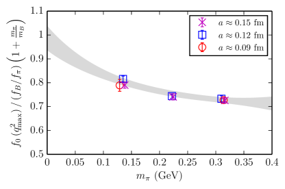
Figure 3: Results for the ratio $R_{B\pi}$ (eq. (24)) of form factor $f_{0}(q^{2}_{max})$ (multiplied by $(1+m_{\pi}/m_{B})$) to $f_{B}/f_{\pi}$, plotted as a function of $m_{\pi}$. Results from very coarse ensembles are shown as crosses, coarse as open squares and fine as open circles. These include a small correction for finite volume effects, as discussed in the text. The grey band shows the fit described in the text, agreeing with value 1 at $m_{\pi}=0$.

In order to test the soft pion theorem we need to fit our results as a function of $m_{\pi}$ to extrapolate to $m_{\pi}=0$. Having results for a range of small $m_{\pi}$ values allows us to do this.

One key element of $m_{\pi}$ dependence is purely kinematic Bowler et al. (2000): the fact that $q^{2}_{\mathrm{m}ax}$ depends on $m_{\pi}$ through the formula

$$q^{2}_{\mathrm{m}ax}=(m_{B}-m_{\pi})^{2}.$$ (25)

This will mean that, if results for different $m_{\pi}$ fall on similar $f_{0}$ curves as a function of $q^{2}$, there will be a significant linear term in $m_{\pi}$ coming from the shift in $q^{2}_{\mathrm{m}ax}$ as $m_{\pi}$ is reduced. A slope in $m_{\pi}$ of order $-2m_{B}df_{0}/dq^{2}|_{q^{2}=q^{2}_{\mathrm{m}ax}}$ might then be expected. An estimate for this slope can be derived from a simple pole form for $f_{0}(q^{2})$, behaving as $f_{0}(0)/[1-q^{2}/m^{2}_{B^{*}_{0}}]$, where the $B^{*}_{0}$ is the lowest scalar state in the $B$ meson spectrum. This would give a slope in $m_{\pi}$ of $f_{0}(q^{2}_{max})/\Lambda$ where $\Lambda$ is the difference in mass between the $B^{*}_{0}$ and the $B$. Taking $\Lambda$ of order 500 MeV results in a slope of 2 $\mathrm{GeV}^{-1}$. The term in $m_{\pi}^{2}$ coming from the kinematics above would have a much smaller slope, of $\mathcal{O}(1/(2\Lambda m_{B}))$, since there is no enhancement by $m_{B}$. This slope is then smaller than that for powers of $m_{\pi}$ coming from chiral perturbation theory and so can be absorbed into those terms in our fit.

From low-order chiral perturbation theory we expect simple powers of $m_{\pi}^{2}$ as well as chiral logarithms of the form $m_{\pi}^{2}/(4\pi f_{\pi})^{2}\times\log(m^{2}_{\pi}/\Lambda^{2}_{\chi})$ (where we take $f_{\pi}=$ 130 MeV). The appropriate staggered quark chiral perturbation theory for these quantities is given in Aubin and Bernard (2003a, 2006, 2007), see also Becirevic et al. (2003). The way in which the masses of different tastes of $\pi$ meson appear in the chiral logarithm terms and associated ‘hairpins’ is discussed in Appendix A. It turns out that the staggered chiral perturbation theory for $f_{\pi}$ and $f_{B}$ is very like the continuum form, because discretisation effects from the masses of $\pi$ mesons of different taste almost entirely cancel out. Terms of this kind in fact cancel between $f_{0}$ and $f_{B}/f_{\pi}$. This includes in particular all the chiral logarithms with coefficient $g_{B^{*}B\pi}$.

The remaining chiral logarithms that do not cancel in the ratio of $f_{0}(q^{2}_{max})$ and $f_{B}/f_{\pi}$ take the form of an average over tastes, $t$, of $m_{\pi_{G}}^{2}/(4\pi f_{\pi})^{2}\times\log(m^{2}_{\pi,t}/\Lambda^{2}_{\chi})$. Here $m_{\pi_{G}}$ is the mass of the Goldstone $\pi$ meson in the final state, and $m_{\pi,t}$ is the mass of a $\pi$ of taste $t$. $m_{\pi_{G}}\equiv m_{\pi}$ is the expansion parameter for the chiral perturbation theory since its square is proportional to the light quark mass. The masses of the other taste $\pi$ mesons, $m_{\pi,t}$, could contribute discretisation errors to the chiral perturbation theory, when compared to the continuum chiral logarithms, since they differ by $\alpha_{s}^{2}a^{2}$ from $m_{\pi_{G}}$. These discretisation errors would be relatively benign, since the chiral logarithm above vanishes as $m_{u/d}\rightarrow 0$ even at non-zero lattice spacing. In fact, as shown in Appendix A, hairpin diagrams also cancel most of these discretisation effects giving a dependence on $m_{\pi}$ which is almost identical to that of continuum chiral perturbation theory. We therefore use continuum chiral perturbation theory for our extrapolation to $m_{\pi}=0$ but allow for $m_{\pi}$-dependent discretisation errors to include remaining staggered taste-changing effects.

Combining results for $f_{B}$, $f_{\pi}$ and $f_{0}$ gives a coefficient for the chiral logarithm above in $f_{0}f_{\pi}/f_{B}$ of -4. A value of -4 is a substantial coefficient, double that in $f_{\pi}$ for example, and so it might be expected that we need to pay attention to finite-volume effects. We studied these for $f_{\pi}$ on these ensembles in Dowdall et al. (2013b) and found them to be well below 1%, except on set 1 which has the coarsest lattice spacing and is furthest from the physical point and so has very little impact on any fit. Finite-volume corrections were included in that study because they were significant at the level of the statistical errors possible there. Here statistical errors are much larger and we find finite volume effects are not significant. We include double the relative finite volume effect seen in $f_{\pi}$ for the ratio $f_{0}f_{\pi}/f_{B}$ in the values shown in Figure 3. This has negligible impact on the final result at physical $m_{\pi}$ and less than 1% effect on the value at $m_{\pi}=0$.

	$R_{B\pi}$	$R_{B_{s}K}$	$R_{B_{s}\eta_{s}}$
stats/fitting	$1.4$	$0.7$	$0.6$
$a$-dependence	$1.3$	$0.6$	$0.4$
NRQCD systematics	$0.03$	$0.03$	$0.04$
$m_{\pi}$ dependence	$0.5$	$0.2$	$0.1$
$s$ quark tuning	-	$0.03$	$0.01$
Total (%)	$1.9$	$1.0$	$0.7$

Table 7: Errors budgets for the ratios $R_{B\pi}$, $R_{B_{s}K}$ and $R_{B_{s}\eta_{s}}$ (defined in eqs (24), (33) and (31)) evaluated at the physical value of $m_{\pi}$. Uncertainties are given as a percentage of the final answer.

We fit the results for the ratio $R_{B\pi}$ as a function of lattice spacing and $\pi$ meson mass to the following form:

$$R_{B\pi}(a,m_{\pi}) = R_{B\pi}(\mathrm{phys},m_{\pi}=0)\times\left[1\right.$$

$$+ \sum_{j=1,3}c_{j}(a\Lambda)^{2j}+d\delta_{a^{2},m^{2}_{\pi}}$$

$$+ \left(\frac{\Lambda}{m_{b}}\right)^{2}(a\Lambda)^{2}[e_{1}\delta x_{m}+e_{2}(\delta x_{m})^{2}]$$

$$+ \left.\sum_{k=1,4}f_{k}\left(\frac{m_{\pi}}{\Lambda_{\chi}}\right)^{k}-g\left(\frac{m_{\pi}}{4\pi f_{\pi}}\right)^{2}\log{\frac{m_{\pi}^{2}}{\Lambda_{\chi}^{2}}}\right]$$

with $\Lambda_{\chi}$ = 1 GeV. Here the $c_{j}$ coefficients provide for regular discretisation errors which appear for our actions as even powers of $a$ only. We take $\Lambda$ = 400 MeV. The coefficient $d$ provides for light quark mass-dependent discretisation errors, as discussed above; more information on these is given below. The terms with coefficients $e_{1}$ and $e_{2}$ allow for discretisation errors from higher-order terms in the NRQCD action with coefficients that might depend on $am_{b}$. $\delta x_{m}=(am_{b}-2.7)/1.5$, so it varies from -0.5 to 0.5 across the range used here for $am_{b}$. We take $\Lambda/m_{b}=0.1$. The $f_{k}$ coefficients provide for $m_{\pi}$ dependence expected from kinematic effects from the dependence of $q^{2}_{\mathrm{m}ax}$ on $m_{\pi}$ (which includes in particular a linear term in $m_{\pi}$ as discussed above). Any dependence on (even) powers of $m_{\pi}$ from chiral perturbation theory will be subsumed into this dependence. The final term is a chiral logarithm, for which we allow coefficient $g$. As discussed above, we use the continuum form for the chiral logarithm and allow for $m_{\pi}$-dependent discretisation effects from staggered chiral perturbation theory with the $\delta_{a^{2},m_{\pi}^{2}}$ term. Our fits are insensitive to the form that this term takes. We have tried, for example, a form based on discretisation effects from averaging over $\pi$ meson tastes in a logarithm:

$$\delta_{a^{2},m_{\pi}^{2}}=\frac{m_{\pi}^{2}}{(4\pi f_{\pi})^{2}}\log(1+2\delta_{t}/m_{\pi}^{2}).$$ (27)

$\delta_{t}$ is one unit of taste-splitting (see Appendix A). For our final results we in fact use the simpler $\delta_{a^{2},m_{\pi}^{2}}=a^{2}m^{2}_{\pi}$. In neither case does the fit return a significant coefficient for this term.

We take a prior of 0.0(1.0) on almost all coefficients in eq. (III.1). The exceptions are: a prior of 1.0(5) on $R_{B\pi}(\mathrm{phys},m_{\pi}=0)$; a prior of $0.0(3)$ on $c_{1}$, since tree-level $a^{2}$ errors are missing from our action so that the leading term is $\alpha_{s}a^{2}$; a prior of 0.0(5.0) on $f_{1}$ since this linear term in $m_{\pi}$ is expected (from the arguments above) to have a coefficient around 2 $\mathrm{GeV}^{-1}$ from its origin in the $m_{\pi}$ dependence of $q^{2}_{\mathrm{m}ax}$ and a prior of 4.0(1.0) on $g$, the coefficient of the chiral logarithm, which is known up to chiral corrections.

The chiral fit has a $\chi^{2}/{\mathrm{dof}}$ of 0.7 for 8 degrees of freedom and gives the result $R_{B\pi}(\mathrm{phys},m_{\pi}=0)$ = 0.987(51), i.e. 1 in agreement with the soft pion relation of eq. (1) with an uncertainty of 5%. Most of the parameters in the fit are not well determined by the data, except for the linear term in $m_{\pi}$ which has coefficient -2.4(5), in agreement with our expectation. Missing out the chiral logarithm changes things slightly, giving a result 2$\sigma$ below 1 at $m_{\pi}$=0 of 0.92(4). Leaving the chiral logarithm unconstrained, i.e. giving $g$ a prior of 0.0(10.0), results in a fitted value for $g$ of 2(8), i.e. it is not well determined by the results (but also not inconsistent with its expected value).

From the fit we can extract the result at the physical value of the $\pi$ meson mass corresponding to equal mass $u$ and $d$ quarks in the absence of electromagnetism. This is the experimental mass of the $\pi^{0}$, 135 MeV. There we find

$$R_{B\pi}(\mathrm{phys},m_{\pi}=m_{\pi^{0}})=0.805(16).$$ (28)

This is very insensitive to any of the details of the fit because we have results at the physical $\pi$ mass. The error budget for $R_{B\pi}(\mathrm{phys},m_{\pi}=m_{\pi^{0}})$ is given in Table 7. Using our value of $f_{B}$ = 0.186(4) GeV Dowdall et al. (2013a) (for the $m_{u}=m_{d}=m_{l}$ case) and the experimental value for $f_{\pi^{+}}$ = 130.4 MeV, along with $(1+m_{\pi^{0}}/m_{B})$ = 1.0256 gives

$$f_{0}(q^{2}_{max})|_{B\rightarrow\pi}=1.120(22)(24).$$ (29)

The first uncertainty comes from the fit to the ratio $R_{B\pi}$ and includes statistical and fitting errors. The second uncertainty comes from our value for $f_{B}$ and includes uncertainties from missing higher order terms in the current matching. We expect these to be very similar for $f_{0}$, since we have seen this to be the case for currents we have included, so we do not include any additional systematic error specific to $f_{0}$. We find finite-volume effects, as discussed above, to give negligible uncertainty.

Taking instead our value of $f_{B^{+}}$ of 0.184(4) GeV Dowdall et al. (2013a) gives

$$f_{0}(q^{2}_{max})|_{B^{+}\rightarrow\pi^{0}}=1.108(22)(24).$$ (30)

III.2 $B_{s}\rightarrow\eta_{s}$

Set	$V^{(0)}_{nn}(0,0)$	$V^{(1)}_{nn}(0,0)$	$V^{V_{0}}$	$g^{B_{s}\eta_{s}}_{0}(q^{2}_{\mathrm{m}ax})$	$R_{B_{s}\eta_{s}}$
1	1.329(14)	-0.042(2)	1.314(14)	1.886(21)	0.740(8)
2	1.323(10)	-0.042(1)	1.306(10)	1.867(15)	0.743(6)
4	1.325(7)	-0.050(0)	1.267(7)	1.648(9)	0.733(4)
6	1.322(2)	-0.051(0)	1.282(2)	1.652(3)	0.740(1)
8	1.347(6)	-0.066(0)	1.284(6)	1.418(6)	0.742(3)

Table 8: Columns 2 and 3 give ground-state parameters in lattice units $V_{nn}(0,0)$ from our combined 2-point and 3-point fit for $B_{s}\rightarrow\eta_{s}\ell\nu$. $V^{(0)}_{nn}$ corresponds to current $J_{V_{0}}^{(0)}$ and $V^{(1)}_{nn}$ to $J_{V_{0}}^{(1)}$ (see eq. (18)). $J_{V_{0}}^{(2)}$ has equal amplitude to $J_{V_{0}}^{(1)}$ at zero recoil and so is not given separately. In column 4 results are combined as in eq. (17) into an equivalent parameter for the full QCD current, $V_{0}$. Column 5 presents the results as the combination $g^{B_{s}\eta_{s}}_{0}\equiv f_{0}\sqrt{am_{B_{s}}}(1+m_{\eta_{s}}/m_{B_{s}})$ in lattice units and Column 6 gives the ratio $R_{B_{s}\eta_{s}}$ defined in eq. (31).

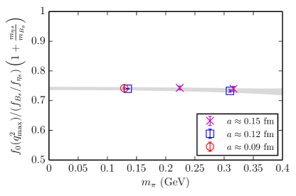
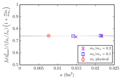
Figure 4: Results for the ratio $R_{B_{s}\eta_{s}}$ of eq. (31) plotted against $m_{\pi}$ in the top plot and against the lattice spacing in the lower plot (see Table 8). The grey band gives the results of a fit described in the text.

The decay mode $B_{s}\rightarrow\eta_{s}$, in which we replace the $l$ quark in $B\rightarrow\pi$ with an $s$ quark is a useful calibration point in lattice QCD. The $\eta_{s}$ meson is a pseudoscalar meson with valence quark content $s\overline{s}$ but including the quark-line-connected correlator only so that it cannot mix with other flavour-singlet mesons. It is thus not a physical particle that appears in experiment. However its properties, mass and decay constant, have been well-studied in lattice QCD Davies et al. (2010); Dowdall et al. (2013b).

The calculation for $B_{s}\rightarrow\eta_{s}$ proceeds exactly as described in Section II for $B\rightarrow\pi$. The valence $s$ quarks have the masses in lattice units given in Table 2. 2-point correlators for the $B_{s}$ and $\eta_{s}$ were calculated in Dowdall et al. (2013a, b). In Table 8 we give the results from this calculation for the 3-point amplitude for $B_{s}\rightarrow\eta_{s}$ decay via a temporal vector current with $B_{s}$ and $\eta_{s}$ at rest. We also give the result derived directly from our fits for the ratio

$$R_{B_{s}\eta_{s}}=\frac{f_{0}(q^{2}_{max})(1+m_{\eta_{s}}/m_{B_{s}})}{[f_{B_{s}}/f_{\eta_{s}}]}.$$ (31)

in which the overall renormalisation of currents cancels. The ratio $R_{B_{s}\eta_{s}}$ is plotted in Figure 4 as a function of the mass of the $\pi$ meson made from the sea $l$ quarks and as a function of the lattice spacing, $a$. We have results only for a subset of the ensembles used for $B\rightarrow\pi$, but we see no dependence of $R_{B_{s}\eta_{s}}$ on either $m_{\pi}$ or on $a$.

To fit the results for $B_{s}\rightarrow\eta_{s}$ decay and derive a physical result for $f_{0}(q^{2}_{\mathrm{m}ax})$ we use a similar fit form to that of eq. (III.1). We drop the chiral logarithm term as well as odd powers of $m_{\pi}$ from kinematic effects, since these are no longer relevant. We add a term allowing for mistuning of the $s$ quark mass as $h(m_{\eta_{s}}^{2}-[0.6885\,\mathrm{GeV}]^{2})$ with prior on h of 0.0(2). Here 0.6885 GeV is the the $\eta_{s}$ mass in the continuum and chiral limits determined from lattice QCD Dowdall et al. (2013b).

Our fit has a $\chi^{2}/{\mathrm{dof}}$ of 0.35 for 5 degrees of freedom and gives a result at physical $m_{\pi}$ for $R_{B_{s}\eta_{s}}$ of 0.740(5). For this quantity the value at $m_{\pi}=0$ has no significance. The physical result for $R_{B_{s}\eta_{s}}$ is very insensitive to any details of the fit since we have results at the physical $\pi$ mass and there is almost no dependence on $m_{\pi}$ and $a$. The error budget is given in Table 7; the uncertainty is dominated by statistics. The value of $R_{B_{s}\eta_{s}}$ can be converted into a value for $f_{0}(q^{2}_{max})$ using $f_{B_{s}}$ = 0.224(5) GeV Dowdall et al. (2013a) and $f_{\eta_{s}}$ = 0.1811(6) GeV and $(1+m_{\eta_{s}}/m_{B_{s}})$ = 1.1283 Dowdall et al. (2013b); Olive et al. (2014). We find

$$\left.f_{0}(q^{2}_{max})\right|_{B_{s}\rightarrow\eta_{s}}=0.811(5)(16)$$ (32)

where the first error is from the ratio and the second from $f_{B_{s}}$ and $f_{\eta_{s}}$. This is a substantially smaller value than that for $B\rightarrow\pi$ and it is also more precise, reflecting smaller statistical uncertainties in the raw data and the absence of any dependence on $m_{\pi}$ or $a$.

III.3 $B_{s}\rightarrow K$

Set	$V^{(0)}_{nn}(0,0)$	$V^{(1)}_{nn}(0,0)$	$V^{V_{0}}$	$g^{B_{s}K}_{0}(q^{2}_{\mathrm{m}ax})$	$R_{B_{s}K}$
1	1.490(8)	-0.060(1)	1.465(8)	1.854(10)	0.656(4)
2	1.510(16)	-0.064(4)	1.481(16)	1.825(20)	0.639(7)
4	1.496(9)	-0.069(1)	1.445(9)	1.654(10)	0.662(4)
6	1.539(8)	-0.075(1)	1.480(8)	1.617(9)	0.623(3)
8	1.571(9)	-0.094(2)	1.483(9)	1.389(9)	0.623(4)

Table 9: Columns 2 and 3 give ground-state parameters in lattice units $V_{nn}(0,0)$ from our combined 2-point and 3-point fit for $B_{s}\rightarrow K\ell\nu$. $V^{(0)}_{nn}$ corresponds to current $J_{V_{0}}^{(0)}$ and $V^{(1)}_{nn}$ to $J_{V_{0}}^{(1)}$ (see eq. (18)). $J_{V_{0}}^{(2)}$ has equal amplitude to $J_{V_{0}}^{(1)}$ at zero recoil and so is not given separately. In column 4 results are combined as in eq. (17) into an equivalent parameter for the full QCD current, $V_{0}$. Column 5 presents the results as the combination $g^{B_{s}K}_{0}\equiv f_{0}\sqrt{am_{B_{s}}}(1+m_{K}/m_{B_{s}})$ in lattice units and Column 6 gives the ratio $R_{B_{s}K}$ defined in eq. (33).

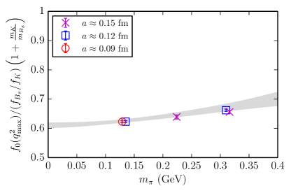
Figure 5: The ratio $R_{B_{s}K}$ of eq. (33) plotted against $m_{\pi}$. See Table 9 for results. The grey band gives the results of a fit described in the text.

The decay mode $B_{s}\rightarrow K\ell\nu$ is a physical process in which a $b$ quark undergoes a weak transition to a $u$ quark inside a $B_{s}$ meson. This process can then be used in a similar way to $B\rightarrow\pi\ell\nu$ to determine $V_{ub}$. Lattice QCD calculations for the form factors for this process are now starting to appear Bouchard et al. (2014); Flynn et al. (2015). Here we again give results for the form factor $f_{0}$ at zero recoil with $u/d$ quark masses going down to physical values. We again study the ratio determined directly from our fits:

$$R_{B_{s}K}=\frac{f_{0}(q^{2}_{max})(1+m_{K}/m_{B_{s}})}{[f_{B_{s}}/f_{K}]}.$$ (33)

Table 9 gives our results and Figure 5 plots the results for $R_{B_{s}K}$ against $m_{\pi}$. We observe no significant $a$ dependence but some dependence on $m_{\pi}$, because the $K$ meson contains a valence $l$ quark. To fit the dependence of $R_{B_{s}K}$ as a function of $m_{\pi}$ and $a$ we use a similar fit form to that used earlier (eq. (III.1)). We drop the odd powers of $m_{\pi}$ from kinematic effects, since these now depend on $m_{K}$ which depends on $m_{l}$ and hence $m^{2}_{\pi}$. As for $B_{s}\rightarrow\eta_{s}$ we add a term allowing for mistuning of the $s$ quark mass as $h(m_{\eta_{s}}^{2}-[0.6885\,\mathrm{GeV}]^{2})$ with prior on h of 0.0(2). We also keep the chiral logarithm term from $B\rightarrow\pi$ but we expect the coefficient to be a lot smaller here so we allow a prior for the coefficient of 0(1). Again, for this quantity, we will only extract a value at the physical value of $m_{\pi}$ (and not $m_{\pi}\rightarrow 0$) and, since we have results very close to that point, the value is insensitive to the details of the fit.

Our fit has a $\chi^{2}/{\mathrm{dof}}$ of 0.2 for 5 degrees of freedom and gives a result at physical $m_{\pi}$ for $R_{B_{s}K}$ of 0.626(6) with error budget given in Table 7. This can be converted into a value for $f_{0}(q^{2}_{max})$ using $f_{B_{s}}$ = 0.224(5) GeV Dowdall et al. (2013a) and $f_{K^{+}}$ = 0.1561 GeV and $(1+m_{K}/m_{B_{s}})$ = 1.0927 Olive et al. (2014). We find

$$\left.f_{0}(q^{2}_{max})\right|_{B_{s}\rightarrow K}=0.822(8)(18).$$ (34)

Here the first error is from $R_{B_{s}K}$ and the second from $f_{B_{s}}$.

IV Discussion

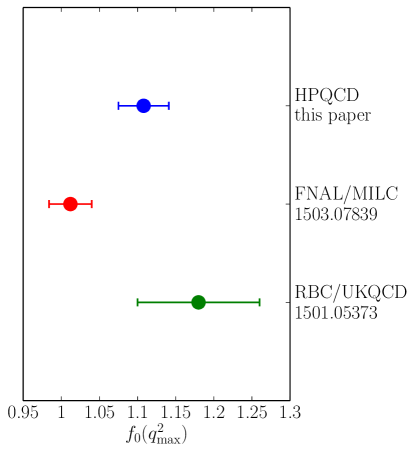
Figure 6: A comparison of results for $f_{0}(q^{2}_{max})$ for $B\rightarrow\pi l\nu$ decay. The top result is from this paper using gluon field configurations that include $u$, $d$, $s$ and $c$ quarks in the sea and include $u/d$ quarks at physical masses. The lower two results Bailey et al. (2015); Flynn et al. (2015) use gluon field configurations that include $u$, $d$ and $s$ quarks in the sea and extrapolate to physical $m_{\pi}$ from heavier values. For all points statistical and systematic uncertainties have been added in quadrature.

We can compare our results for $f_{0}(q^{2}_{max})$ for $B\rightarrow\pi$ and $B_{s}\rightarrow K$ to existing full lattice QCD results where an extrapolation in $m_{\pi}$ to the physical point has been done (as well as a study of $f_{+}$ and $f_{0}$ as a function of $q^{2}$).

Figure 6 shows this comparison for $B\rightarrow\pi$, comparing our result to that from Fermilab/MILC Bailey et al. (2015) and RBC/UKQCD Flynn et al. (2015). Both of these calculations use a ‘clover’ formalism for the $b$ quark, which has a nonrelativistic interpretation on coarse lattices seamlessly matching to a relativistic formulation as $a\rightarrow 0$. Details differ significantly in the two cases El-Khadra et al. (1997); Christ et al. (2007) with the RBC/UKQCD calculation tuning the clover term nonperturbatively and including $\mathcal{O}(\alpha_{s}a)$ current corrections to reduce discretisation errors. The Fermilab/MILC results couple their $b$ quark to an asqtad staggered quark on the MILC 2+1 asqtad configurations. They cover a range of lattice spacing values from 0.12 fm to 0.045 fm and have a minimum light quark mass corresponding to a value for $m_{\pi}$ of 180 MeV on 0.09 fm lattices. The RBC/UKQCD results use domain-wall light quarks on their 2+1 domain-wall configurations with two lattice spacing values (0.11 fm and 0.086 fm) and a minimum light quark mass corresponding to a value for $m_{\pi}$ of 290 MeV.

As discussed above, our results have the advantage of including much lower values of $m_{l}$, down to values of physical $m_{\pi}$ (indeed our maximum light quark mass corresponds to $m_{\pi}$ of 305 MeV) as well as using a more highly-improved action (to reduce discretisation errors) for both the $b$ quark, the light quark, the current connecting them, and the gluon field.

We see agreement between our result and that from RBC/UKQCD within their larger uncertainties. There is a 2$\sigma$ ‘tension’ between our result and that of Fermilab/MILC where we have similar 3% uncertainties. The Fermilab/MILC value for $f_{0}(q^{2}_{max})$ for $B^{+}\rightarrow\pi^{0}$ is 1.012(28) Zhou (2015) to be compared to our result of 1.108(33) (eq. 30) for the same case.

For the processes $B_{s}\rightarrow K$ and $B_{s}\rightarrow\eta_{s}$ the extrapolation in $m_{\pi}$ is less of an issue and instead, for example, it becomes important to tune the $s$ quark mass accurately. For our $B_{s}\rightarrow K$ result we can compare to RBC/UKQCD as above Flynn et al. (2015) and also to an earlier HPQCD result Bouchard et al. (2014) (which also gives $B_{s}\rightarrow\eta_{s}$ form factors). This latter result uses $\mathcal{O}(v^{4})$ NRQCD for the $b$ quark with HISQ valence light quarks on MILC 2+1 asqtad lattices at two lattice spacing values (0.12 fm and 0.09 fm) and with a minimum light sea quark mass corresponding to $m_{\pi}$ = 280 MeV. In all cases we see agreement with our results, given in eqs (32) and (34), within the larger $\mathcal{O}(5\%)$ uncertainties of Flynn et al. (2015); Bouchard et al. (2014). For example Flynn et al. (2015) quotes a result for $f_{0}$ for $B_{s}\rightarrow K$ at $q^{2}=23.4\mathrm{GeV}^{2}$ of 0.81(6) to be compared to our result at $q^{2}_{max}$ of 23.7 $\mathrm{GeV}^{2}$ of 0.822(20) (eq. (34)).

In the comparison of $B/B_{s}$ semileptonic form factors to experiment for extraction of $V_{ub}$ it should be emphasised that it is the $f_{+}$ form factor that is relevant for $\mu\nu$ or $e\nu$ final states, and not $f_{0}$. However, similar issues arise in both cases for the extrapolation to physical $m_{\pi}$ and so the tests above for $f_{0}$ are also relevant to $f_{+}$.

V Conclusions

In this paper we have laid to rest a long-standing controversy over the relationship between the form factor $f_{0}$ at zero recoil in $B\rightarrow\pi$ decay and the ratio $f_{B}/f_{\pi}$ from lattice QCD results. We calculate the ratio of $f_{0}$ to $f_{B}/f_{\pi}$ directly and obtain particularly accurate results because:

• our lattice $b$-light currents are accurate through $\alpha_{s}\Lambda/m_{b}$ and the renormalisation of the current cancels between $f_{0}$ and $f_{B}$.

• we work with light quarks that have their physical mass as well as heavier masses to allow an extrapolation to $m_{\pi}=0$. This is well controlled because of the form the staggered quark chiral perturbation theory takes (see Appendix A).

• we use improved actions for our $b$ quarks, light quarks and gluon fields, so that discretisation errors are reduced below $\alpha_{s}a^{2}$.

We find

$$\left.\frac{f^{B\rightarrow\pi}_{0}(q^{2}_{max})}{f_{B}/f_{\pi}}\right|_{m_{\pi}=0}=0.987(51)$$ (35)

in agreement with the soft-pion theorem result of 1. This test adds confidence to our control of lattice systematic uncertainties now that we have reached values of the $\pi$ mass close to the physical point.

We are then able to determine values of the $f_{0}$ form factor at zero recoil and for physical quark masses for 3 processes, obtaining the ratios defined in Section II:

$$R_{B\pi}(\mathrm{phys})=0.805(16)$$

$$R_{B_{s}K}(\mathrm{phys})=0.626(6)$$

$$R_{B_{s}\eta_{s}}(\mathrm{phys})=0.740(5).$$ (36)

Numbers vary by 30% as the quark content in initial and final state changes between $l$ and $s$, with corresponding changes in the value of $q^{2}_{\mathrm{max}}$. This allows us to extract:

$$\left.f_{0}(q^{2}_{max})\right|_{B^{+}\rightarrow\pi^{0}} = 1.108(22)(24)$$

$$\left.f_{0}(q^{2}_{max})\right|_{B_{s}\rightarrow K} = 0.822(8)(18)$$

$$\left.f_{0}(q^{2}_{max})\right|_{B_{s}\rightarrow\eta_{s}} = 0.811(5)(16).$$ (37)

These can act as calibration values for lattice QCD calculations working at heavier-than-physical light quark masses. The uncertainties we have reached in this first ‘second-generation’ form-factor calculation are encouraging for the improvements that will be possible as we move away from zero recoil.

Acknowledgements We are grateful to the MILC collaboration for the use of their configurations, to R. Horgan, C.Monahan and J. Shigemitsu for calculating the pieces needed for the current renormalisation used here, and to R. Zhou for useful discussions on the Fermilab/MILC results. Computing was done on the Darwin supercomputer at the University of Cambridge as part of STFC’s DiRAC facility. We are grateful to the Darwin support staff for assistance. Funding for this work came from STFC, the Royal Society and the Wolfson Foundation.

Appendix A Why are staggered quarks so continuum-like?

The $\not{D}$ operator in staggered-quark lattice discretisations has $\mathcal{O}(a^{2})$ lattice-spacing corrections that do not vanish in the limit of zero quark mass $m_{q}$. These are due to taste-changing interactions and affect the zero modes of the lattice Dirac operator $i\not{D}+m_{q}$ in the chiral limit, altering the topological properties of the theory at non-zero lattice spacing Follana et al. (2004, 2005). In principle, therefore, one should take the continuum limit $a\to 0$ before taking the chiral limit $m_{q}\to 0$; that is, there will be a smallest quark mass for each lattice spacing below which non-physical effects will show up.

In practice, these non-physical effects have been small, especially with the HISQ discretisation and similar actions designed to suppress taste-changing interactions Lepage (1999). Such possibilities have therefore had minimal effect on analyses of meson decay constants and masses (see, for example, Dowdall et al. (2013b)). This might seem surprising because we are now working at realistic $u/d$ quark masses which are very small. Here we are also examining the limit as $m_{\pi}\rightarrow 0$ (based on results at non-zero values of $m_{\pi}$ and $a$).

Chiral perturbation theory, and, in particular, staggered chiral perturbation theory is a useful tool for analyzing such effects. The problem is then apparent from the fact that the masses of different tastes of pion are split by taste-changing interactions of $\mathcal{O}(a^{2}\alpha_{s}^{2},a^{2}\alpha_{s}^{3})$, so that only the Goldstone pion’s mass vanishes when the quark mass goes to zero. This affects the chiral logarithms in the theory since these typically involve averages over the masses of all tastes of pion in staggered chiral perturbation theory. As long as taste-splittings are small compared to the Goldstone pion mass then the difference is purely a discretisation effect. However, in the opposite limit of $m_{\pi}\to 0$, $m_{\pi}^{2}\log(m_{\pi}^{2})$ in the continuum theory is replaced by $a^{2}\log(a^{2})$ in the staggered-quark theory. While such terms vanish as $a\to 0$, one might still worry that unusually large $a^{2}$ corrections and corrections that are not analytic in $a^{2}$ would make the approach to the continuum limit hard to control in practice, as well as distorting the $m_{\pi}$ dependence.

In fact, as we show here, the leading non-analyticities in $a^{2}$ cancel as $m_{u/d}\to 0$ when using the HISQ discretisation at current lattice spacings, at least for such phenomenologically important quantities as: $f_{\pi}$, $m_{\pi}^{2}$, $f_{K}$, $f_{B}$ and $f_{0}^{B\rightarrow\pi}$. Consequently HISQ quarks are more continuum-like in their $a$ and $m_{\pi}$ dependence than might have been expected, even for very small $u/d$ masses.

The non-analytic $a^{2}$ dependence coming from the normal chiral logarithms is cancelled by contributions from the ‘hairpin’ diagrams in staggered chiral perturbation theory. We will show how this cancellation works in the next subsection. The cancellation occurs only for special values of the staggered chiral theory parameters $\delta_{V}^{\prime}$ and $\delta_{A}^{\prime}$, but at the same values for each of the physical quantities mention above. Simulations show that the actual values are within 10% or so of the special values required for cancellation.

A.1 Staggered Chiral Perturbation Theory analysis

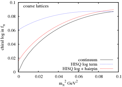
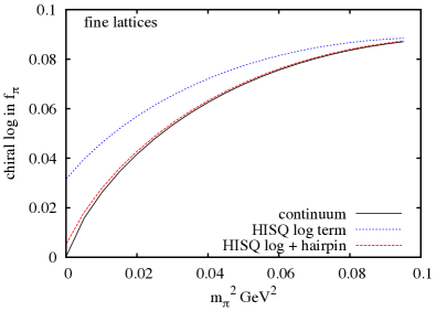
Figure 7: The chiral logarithm term in $m_{\pi}$ that appears in the chiral expansion of $f_{\pi}$ is shown as a function of $m_{\pi}$ in the continuum (solid black line) and compared to the results for the HISQ action from staggered chiral perturbation theory including logarithms and ‘hairpin’ terms (red dashed line). The blue dotted lines shows results if only the ‘staggered’ chiral logarithm is included. Results appropriate to our coarse lattices are shown in the upper plot, with results for the fine lattices in the lower plot.

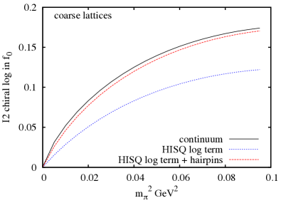
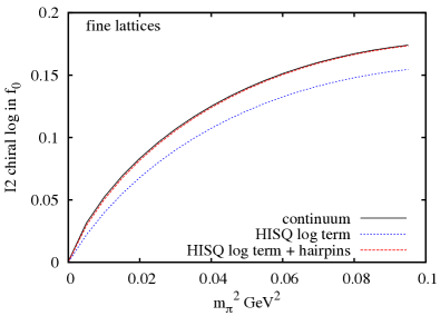
Figure 8: The chiral logarithm denoted $I2$ that appears in the chiral expansion of $f^{B\rightarrow\pi}_{0}(q^{2}_{max})$ is shown as a function of $m_{\pi}$ in the continuum (solid black line) and compared to the results for the HISQ action from staggered chiral perturbation theory including logarithms and ‘hairpin’ terms (red dashed line). The blue dotted lines shows results if only the ‘staggered’ chiral logarithm is included. Results appropriate to our coarse lattices are shown in the upper plot, with results for the fine lattices in the lower plot.

As examples, we first study $f_{\pi}$, $f_{K}$ and $f_{B}$ in the 2+1 full QCD case using formulae from Aubin and Bernard (2003a) (eqs. 27 and 28) and Aubin and Bernard (2006) (eq. 105). We will evaluate here the leading behaviour in $a$ at Goldstone $m_{\pi}=0$ ($m_{u/d}=0$). The key terms are those that contain logarithms of masses of different tastes of pion - different tastes of kaon or other strange particle are irrelevant because their masses will be controlled by the $s$ quark mass.

We implement a model for different tastes of pion in which the tastes are equally spaced. This is a very good approximation to what happens in simulations with the Highly Improved Staggered Quark action Bazavov et al. (2013) (and indeed the asqtad improved staggered quark action). This is an indication that the taste-breaking potential in the staggered chiral Lagrangian is dominated by one particular term Lee and Sharpe (1999); Aubin and Bernard (2003b); Follana et al. (2007). If we take the unit of splitting to be $\delta_{t}$ (proportional to $\alpha^{2}a^{2}$ or even $\alpha^{3}a^{2}$ in an improved formalism) then the Goldstone (G) pion mass will be zero when $m_{u/d}=0$ and the other tastes (axial vector, tensor, vector and singlet) will have squared masses according to:
$G:0$
$A:\delta_{t}$
$T:2\delta_{t}$
$V:3\delta_{t}$
$I:4\delta_{t}$.
The degeneracies of the different tastes from the Goldstone upwards in mass are: 1, 4, 6, 4, 1, making a total of 16 tastes.

Then we can evaluate the chiral log terms that appear in the NLO term multiplying $1/(16\pi^{2}f^{2})$ in staggered chiral perturbation theory at $m_{u/d}=0$. For $f_{\pi}$ this is simply:

$$-\frac{1}{8}\sum_{t}m_{\pi,t}^{2}\log{m_{\pi,t}^{2}} = -\frac{1}{8}(4\delta_{t}\log\delta_{t}+12\delta_{t}\log 2\delta_{t}$$ (38)

$$+12\delta_{t}\log 3\delta_{t}+4\delta_{t}\log 4\delta_{t})$$

$$= -4\delta_{t}\log\delta_{t}+C\delta_{t}$$

where $C$ is a constant. The $C\delta_{t}$ term is then a normal discretisation error which we will ignore here. Similarly for $f_{K}$ and $f_{B}$ (which has an overall extra factor of $1+3g_{B^{*}B\pi}^{2}$) the log term appears as:

$$-\frac{1}{16}\sum_{t}m_{\pi,t}^{2}\log{m_{\pi,t}^{2}}+\frac{1}{4}m_{\pi,I}^{2}\log{m_{\pi,I}^{2}}=$$ (39)

$$-\frac{1}{16}\left(4\delta_{t}\log\delta_{t}+12\delta_{t}\log 2\delta_{t}+12\delta_{t}\log 3\delta_{t}\right.$$

$$+\left.4\delta_{t}\log 4\delta_{t}\right)+\delta_{t}\log 4\delta_{t}$$

$$= -\delta_{t}\log\delta_{t}+C\delta_{t}$$

Thus it is clear that the chiral logarithm terms on their own will give rise to potentially troublesome $\delta_{t}\log\delta_{t}\equiv a^{2}\log a^{2}$ terms (ignoring $\alpha_{s}$ factors in $\delta_{t}$ although in practice they make a significant numerical difference) as $m_{u/d}\rightarrow 0$.

In addition there are ‘hairpin’ terms at NLO that come in a variety of forms. The key ones that can contain terms of the form $a^{2}\log a^{2}$ as $m_{u/d}\rightarrow 0$ are those multiplying logarithms of the mass of a taste of pion or a taste of $\eta$ (but not the singlet). For $f_{\pi}$ there are two such hairpin terms that we reproduce here in the axial taste case (there is also a vector taste version of them) Aubin and Bernard (2003a). Term 1 is :

$$T1=\frac{(m^{2}_{S_{A}}-m^{2}_{\eta_{A}})}{(m^{2}_{\pi_{A}}-m^{2}_{\eta_{A}})(m^{2}_{\eta^{\prime}_{A}}-m^{2}_{\eta_{A}})}\ell(m_{\eta_{A}})$$ (40)

where $\ell(m)=m^{2}\log m^{2}$ and this term appears with coefficient $2\delta_{A}^{\prime}$ which is itself $\mathcal{O}(a^{2})$ (we absorb the $a^{2}$ into $\delta_{A}^{\prime}$ here).

To evaluate $T1$ we use Aubin and Bernard (2003b):

$$m^{2}_{\eta_{A}} = \frac{1}{2}(m^{2}_{\pi_{A}}+m^{2}_{S_{A}}+0.75\delta_{A}^{\prime}-Z)$$

$$m^{2}_{\eta^{\prime}_{A}} = \frac{1}{2}(m^{2}_{\pi_{A}}+m^{2}_{S_{A}}+0.75\delta_{A}^{\prime}+Z)$$ (41)

$$Z=$$

$$\sqrt{(m^{2}_{S_{A}}-m^{2}_{\pi_{A}})^{2}-0.5\delta_{A}^{\prime}(m^{2}_{S_{A}}-m^{2}_{\pi_{A}})+9(\delta_{A}^{\prime})^{2}/16}$$

where $m^{2}_{S_{A}}$ is the axial taste of the $s\overline{s}$ pseudoscalar which we take to have the same taste-splittings as the pion. Again this is a very good approximation in the HISQ case Bazavov et al. (2013).

We can evaluate $Z$ to first order in $\delta_{A}^{\prime}$ at $m_{u/d}=0$ as:

$$Z=(m^{2}_{S_{A}}-m^{2}_{\pi_{A}})-\delta_{A}^{\prime}/4$$ (43)

and then the $\eta$ and $\eta^{\prime}$ masses follow:

$$m^{2}_{\eta_{A}} = m^{2}_{\pi_{A}}+\delta_{A}^{\prime}/2$$ (44)

$$m^{2}_{\eta^{\prime}_{A}} = m^{2}_{S_{A}}+\delta_{A}^{\prime}/4$$

Then we can evaluate each of the mass differences in $T1$:

$$m^{2}_{\eta^{\prime}_{A}}-m^{2}_{\eta_{A}} = Z$$

$$= m^{2}_{S_{G}}-\delta_{A}^{\prime}/4$$

$$m^{2}_{S_{A}}-m^{2}_{\eta_{A}}=m^{2}_{S_{G}}-\delta_{A}^{\prime}/2$$ (46)

$$m^{2}_{\pi_{A}}-m^{2}_{\eta_{A}}=-\delta_{A}^{\prime}/2.$$ (47)

This final mass difference, appearing in the denominator of $T1$ looks dangerous but the whole term, as discussed above, is multiplied by $\delta_{A}^{\prime}$.

Combining all the mass differences we have:

$$2\delta_{A}^{\prime}T1 = 2\delta_{A}^{\prime}\frac{m^{2}_{S_{G}}}{(-\delta_{A}^{\prime}/2)m^{2}_{S_{G}}}\ell(m_{\eta_{A}})$$ (48)

$$= -4m^{2}_{\eta_{A}}\log m^{2}_{\eta_{A}}$$

to leading order in $\delta_{A}^{\prime}$. However $\delta_{A}^{\prime}$ still appears inside $m^{2}_{\eta_{A}}$.

We approach $T2$ similarly.

$$T2=\frac{(m^{2}_{S_{A}}-m^{2}_{\pi_{A}})}{(m^{2}_{\eta_{A}}-m^{2}_{\pi_{A}})(m^{2}_{\eta^{\prime}_{A}}-m^{2}_{\pi_{A}})}\ell(m_{\pi_{A}})$$ (49)

From above we have the mass differences:

$$m^{2}_{\eta^{\prime}_{A}}-m^{2}_{\pi_{A}} = m^{2}_{S_{G}}+\delta_{A}^{\prime}/4$$ (50)

$$m^{2}_{\eta_{A}}-m^{2}_{\pi_{A}} = +\delta_{A}^{\prime}/2$$

$$m^{2}_{S_{A}}-m^{2}_{\pi_{A}} = m^{2}_{S_{G}}$$

Then

$$2\delta_{A}^{\prime}T2 = 2\delta_{A}^{\prime}\frac{m^{2}_{S_{G}}}{(\delta_{A}^{\prime}/2)m^{2}_{S_{G}}}\ell(m_{\pi_{A}})$$ (51)

$$= 4m^{2}_{\pi_{A}}\log m^{2}_{\pi_{A}}$$

Adding $T1$ and $T2$, as required for the chiral expansion of $f_{\pi}$ gives:

$$4(m^{2}_{\pi_{A}}\log m^{2}_{\pi_{A}}-m^{2}_{\eta_{A}}\log m^{2}_{\eta_{A}})$$

$$= 4(\delta_{t}\log\delta_{t}-(\delta_{t}+\delta_{A}^{\prime}/2)\log(\delta_{t}+\delta_{A}^{\prime}/2))$$

Since $\delta_{A}^{\prime}$ also arises from staggered-quark taste effects we can assume that it is some multiple of the unit of taste-splitting, $\delta_{t}$. If we write it as a multiple, $x_{A}$, of the largest taste-splitting (between the taste-singlet and the Goldstone), then $\delta_{A}^{\prime}=4x_{A}\delta_{t}$. The sum of $T1$ and $T2$ becomes

$$4(\delta_{t}\log\delta_{t} - (1+2x_{A})\delta_{t}\log(1+2x_{A})\delta_{t})$$

$$= 4(1-(1+2x_{A}))\delta_{t}\log\delta_{t}+C\delta_{t}$$

$$= -8x_{A}\delta_{t}\log\delta_{t}$$

neglecting terms of $\mathcal{O}(\delta_{t})$. An equivalent result would be obtained for the vector hairpin terms.

Combining the chiral log for $f_{\pi}$ with the $\delta_{A}^{\prime}$ and $\delta_{V}^{\prime}$ hairpin terms then gives:

$$-4\delta_{t}\log\delta_{t} - 8(x_{A}+x_{V})\delta_{t}\log\delta_{t}=$$

$$-4(1+2[x_{A}+x_{V}])\delta_{t}\log\delta_{t}$$

We see that $x_{A}+x_{V}=-0.5$ is a special value where the $\delta_{t}\log\delta_{t}$ (i.e. $a^{2}\log a^{2}$) terms cancel between the chiral logarithms and the hairpins. In fact this is the value that is obtained from staggered chiral perturbation theory fits to $f_{\pi}$ and $f_{K}$. Such fits in Dowdall et al. (2013b) give

$$x_{A} = -0.31(4)$$ (55)

$$x_{V} = -0.25(6)$$

so that $\delta_{A}^{\prime}\approx\delta_{V}^{\prime}\approx-\delta_{t}$. Then the axial taste of $\eta$ has a mass between that of the Goldstone and axial tastes of pion from eq. (47).

The impact of this is made clear in Figure 7 in which we plot the chiral logarithm term as a function of the (Goldstone) $m_{\pi}$. The solid black curve shows the continuum form $-2(m_{\pi}^{2}/\Lambda_{\chi}^{2})\log(m_{\pi}^{2}/\mu^{2})$ with $\Lambda_{\chi}=4\pi f_{\pi}$ (for $f_{\pi}$ = 130 MeV) and $\mu=0.568$ GeV. For comparison we show the result from simply replacing the continuum chiral logarithm by an average over chiral logarithms for each taste of pion (the term analysed in eq. (38)). We take equally-spaced masses for the tastes with splittings appropriate to coarse and fine lattices from Bazavov et al. (2013). The distortion of the continuum chiral logarithm from taste-splitting discretisation effects is clear, particularly on the coarse lattices at small values of $m_{\pi}$. In contrast, when the complete staggered chiral perturbation theory expression is taken, including the hairpin corrections discussed above, the taste-splitting discretisation effects are almost eliminated and the match with the continuum chiral perturbation theory behaviour is restored. The curves in Figure 7 used $\delta_{A}^{\prime}=\delta_{V}^{\prime}=-\delta_{t}$ with $\delta_{t}=0.022\,\mathrm{GeV}^{2}$ on coarse lattices and $\delta_{t}=0.007\,\mathrm{GeV}^{2}$ on fine lattices. The impact of taste-changing discretisation effects on the chiral perturbation theory is then very small, even on the coarse lattices.

To understand why the full staggered chiral perturbation theory looks so continuum-like across the full range of $m_{\pi}$ values (and not just as $m_{\pi}\rightarrow 0$) we can consider another limit in which $\delta_{t}<m_{\pi}^{2}$ with $0<m_{\pi}^{2}<m_{\eta_{s}}^{2}$. This region is in reasonable correspondence with the right-hand side of our plots in Figure 7. Then the full staggered chiral perturbation theory gives the continuum chiral logarithms as well as terms that behave as $\delta_{t}\log m_{\pi}^{2}$ and $m_{\pi}^{2}\log(1+n\delta_{t}/m_{\pi}^{2})\equiv n\delta_{t}$. Both of these terms look like regular discretisation errors and are not problematic. However, once again, both of these terms cancel between the staggered chiral logarithms and the hairpin terms for the case above where $\delta_{A}^{\prime}=\delta_{V}^{\prime}=-\delta_{t}$. This explains why there is such good correspondence, with only very small discretisation errors visible, between the full staggered chiral perturbation theory and the continuum chiral logarithm for $f_{\pi}$ across the full range of $m_{\pi}^{2}$ values in Figure 7.

The staggered chiral perturbation theory for $f_{K}$ and $f_{B}$ is similar to that for $f_{\pi}$ Aubin and Bernard (2003a, 2006). The hairpin contributions that can give $a^{2}\log a^{2}$ terms as $m_{\pi}^{2}\rightarrow 0$ in these cases are identical to the $T1$ and $T2$ above for $f_{\pi}$ (eqs. (40) and (49)). They come with a coefficient of $1/2$ instead of 2, however (again $f_{B}$ has the additional multiplier of $1+3g^{2}_{B^{*}B\pi}$). This is exactly the overall factor of $1/4$ needed to cancel the $\delta_{t}\log\delta_{t}$ piece of the chiral logarithm (eq. (39)) when $x_{A}+x_{V}=-0.5$ as for $f_{\pi}$. So again in this case staggered chiral perturbation theory behaves much more benignly than might be expected in its approach to the continuum limit. This will also be true, as for $f_{\pi}$, across our range of $m_{\pi}$ values.

The staggered chiral perturbation theory for $m_{\pi}$ (in terms of $m_{u/d}$) is somewhat different from the examples above Aubin and Bernard (2003b). The ‘chiral log’ is simply $\ell(m_{\pi_{I}})$. For $m_{u/d}=0$ this becomes $4\delta_{t}\log 4\delta_{t}$ multiplying the standard factor of $1/(16\pi^{2}f^{2})$.

The ‘hairpin’ terms are also somewhat different. For the axial case, keeping only the pieces that can give rise to $\delta_{t}\log\delta_{t}$ terms, we have:

$$T3 = -4\ell(m_{\pi_{A}})$$ (56)

$$- \frac{2\delta_{A}^{\prime}}{m^{2}_{\eta^{\prime}_{A}}-m^{2}_{\eta_{A}}}\frac{m^{2}_{S_{A}}-m^{2}_{\eta_{A}}}{m^{2}_{\pi_{A}}-m^{2}_{\eta_{A}}}\ell(m_{\eta_{A}})$$

Using mass-splittings from above this becomes

$$T3 = -4\ell(m_{\pi_{A}})-2\delta_{A}^{\prime}\frac{m^{2}_{S_{G}}}{m^{2}_{S_{G}}(-\delta_{A}^{\prime}/2)}\ell(m_{\eta_{A}})$$ (57)

$$= -4\ell(m_{\pi_{A}})+4\ell(m_{\eta_{A}})$$

This shows how the $\log m_{\pi}$ factors in the $a\rightarrow 0$ limit cancel between the two halves of T3. To obtain the $a^{2}\log a^{2}$ pieces as $m_{u/d}\rightarrow 0$ we need to take the Goldstone $m_{\pi}$ to zero. Then we have, for the axial case:

$$T3 = -4\delta_{t}\log\delta_{t}+4(1+2x_{A})\delta_{t}\log(1+2x_{A})\delta_{t}$$ (58)

$$= 8x_{A}\delta_{t}\log\delta_{t}$$

Again, adding in the vector taste piece, we find that the value $x_{A}+x_{V}=-0.5$ cancels the $\delta_{t}\log\delta_{t}$ behaviour from the chiral log term above. So the same values for the $\delta_{A}^{\prime}$ and $\delta_{V}^{\prime}$ coefficients also give rise here to a cancellation of taste-splitting artefacts in the staggered chiral perturbation theory. It is also true, as before, that this cancellation can be demonstrated explicitly for the $m_{\pi}^{2}>0$ case when $\delta_{t}<m_{\pi}^{2}$ and in practice numerically it works across the whole $m_{\pi}$ range used here.

For the form-factor $f_{0}^{B\rightarrow\pi}$ discussed here we use the staggered chiral perturbation theory given in Aubin and Bernard (2007) (eq.67). Not surprisingly a set of terms appear there containing logarithms of $m^{2}_{\pi,t}$ that are the same as those appearing in the staggered chiral perturbation theory for $f_{\pi}$ and $f_{B}$. Our analysis above then demonstrates that these terms (combining chiral logarithms and hairpins) behave as continuum chiral perturbation theory. In fact these terms (denoted by $I_{1}$ in Aubin and Bernard (2007)) cancel between $f_{0}$ and $f_{B}/f_{\pi}$ in the ratio $R_{B\pi}$ that we consider here.

There are additional terms in $f_{0}$ denoted $I_{2}$ in Aubin and Bernard (2007) that also behave as chiral logarithms. They have the form $(v.p)^{2}\log(m^{2}_{\pi,t}/\mu^{2})$ where $v.p$ is the dot product of $B$ meson velocity and $\pi$ 4-momentum. For a $B$ meson at rest and a Goldstone $\pi$ in the final state this gives $E^{2}_{\pi,G}\log(m^{2}_{\pi,t}/\mu^{2})$, reducing to $m^{2}_{\pi,G}\log(m^{2}_{\pi,t}/\mu^{2})$ at zero recoil. These are the chiral logarithm terms that survive in the ratio $R_{B\pi}$ and that we include in our fit of eq. (III.1). Such terms only contain $\delta_{t}$ inside the logarithm and so cannot give rise to $\delta_{t}\log\delta_{t}$ terms. The approach to $m_{\pi}\equiv m_{\pi,G}=0$ for $R_{B\pi}$ is therefore the same as in continuum chiral perturbation theory even at non-zero lattice spacing. Discretisation effects could arise from the $m^{2}_{\pi,t}$ inside the logarithm but these can be shown to cancel in the $\delta_{t}<m_{\pi}^{2}$ case for the same $\delta_{A}^{\prime}$ and $\delta_{V}^{\prime}$ values (in eq. (55). Once again the numerical result, shown in Fig. 8, gives continuum-like behaviour for the staggered chiral perturbation across the full range of $m_{\pi}$ values. We nevertheless allow for possible $m_{\pi}$-dependent discretisation errors in our chiral fit, as discussed in Section III.

References

- Bailey et al. (2015) J. A. Bailey et al. (Fermilab Lattice, MILC collaborations), Phys. Rev. D92, 014024 (2015), eprint 1503.07839.
- Flynn et al. (2015) J. M. Flynn, T. Izubuchi, T. Kawanai, C. Lehner, A. Soni, R. S. Van de Water, and O. Witzel, Phys. Rev. D91, 074510 (2015), eprint 1501.05373.
- Onogi (1998) T. Onogi, Nucl. Phys. Proc. Suppl. 63, 59 (1998), eprint hep-lat/9802027.
- Hashimoto (2000) S. Hashimoto, Nucl.Phys.Proc.Suppl. 83, 3 (2000), eprint hep-lat/9909136.
- Dominguez et al. (1990) C. A. Dominguez, J. G. Korner, and K. Schilcher, Phys. Lett. B248, 399 (1990).
- Wise (1992) M. B. Wise, Phys. Rev. D45, 2188 (1992).
- Burdman and Donoghue (1992) G. Burdman and J. F. Donoghue, Phys. Lett. B280, 287 (1992).
- Wolfenstein (1992) L. Wolfenstein, Phys. Lett. B291, 177 (1992).
- Burdman et al. (1994) G. Burdman, Z. Ligeti, M. Neubert, and Y. Nir, Phys. Rev. D49, 2331 (1994), eprint hep-ph/9309272.
- Dowdall et al. (2013a) R. Dowdall, C. Davies, R. Horgan, C. Monahan, and J. Shigemitsu (HPQCD Collaboration), Phys.Rev.Lett. 110, 222003 (2013a), eprint 1302.2644.
- Dowdall et al. (2013b) R. Dowdall, C. Davies, G. Lepage, and C. McNeile (HPQCD Collaboration), Phys.Rev. D88, 074504 (2013b), eprint 1303.1670.
- Bazavov et al. (2013) A. Bazavov et al. (MILC Collaboration), Phys.Rev. D87, 054505 (2013), eprint 1212.4768.
- Follana et al. (2007) E. Follana, Q. Mason, C. Davies, K. Hornbostel, G. P. Lepage, et al. (HPQCD Collaboration), Phys.Rev. D75, 054502 (2007), eprint hep-lat/0610092.
- Hart et al. (2009) A. Hart, G. von Hippel, and R. Horgan (HPQCD Collaboration), Phys.Rev. D79, 074008 (2009), eprint 0812.0503.
- Dowdall et al. (2012a) R. Dowdall, B. Colquhoun, J. O. Daldrop, C. T. H. Davies, et al. (HPQCD Collaboration), Phys.Rev. D85, 054509 (2012a), eprint 1110.6887.
- Olive et al. (2014) K. Olive et al. (Particle Data Group), Chin.Phys. C38, 090001 (2014).
- Lepage et al. (1992) G. P. Lepage, L. Magnea, C. Nakhleh, U. Magnea, and K. Hornbostel, Phys.Rev. D46, 4052 (1992), eprint hep-lat/9205007.
- Hammant et al. (2013) T. Hammant, A. Hart, G. von Hippel, R. Horgan, and C. Monahan, Phys.Rev. D88, 014505 (2013), eprint 1303.3234.
- Colquhoun et al. (2015a) B. Colquhoun, R. J. Dowdall, C. T. H. Davies, K. Hornbostel, and G. P. Lepage (HPQCD Collaboration), Phys. Rev. D91, 074514 (2015a), eprint 1408.5768.
- Gray et al. (2005) A. Gray, I. Allison, C. Davies, E. Dalgic, G. Lepage, et al. (HPQCD Collaboration), Phys.Rev. D72, 094507 (2005), eprint hep-lat/0507013.
- Daldrop et al. (2012) J. Daldrop, C. Davies, and R. Dowdall (HPQCD Collaboration), Phys.Rev.Lett. 108, 102003 (2012), eprint 1112.2590.
- Dowdall et al. (2014) R. Dowdall, C. Davies, T. Hammant, and R. Horgan (HPQCD Collaboration), Phys.Rev. D89, 031502 (2014), eprint 1309.5797.
- Dowdall et al. (2012b) R. Dowdall, C. Davies, T. Hammant, and R. Horgan (HPQCD Collaboration), Phys.Rev. D86, 094510 (2012b), eprint 1207.5149.
- Colquhoun et al. (2015b) B. Colquhoun, C. T. H. Davies, R. J. Dowdall, J. Kettle, J. Koponen, G. P. Lepage, and A. T. Lytle (HPQCD Collaboration), Phys. Rev. D91, 114509 (2015b), eprint 1503.05762.
- Wingate et al. (2003) M. Wingate, J. Shigemitsu, C. T. Davies, G. P. Lepage, and H. D. Trottier, Phys.Rev. D67, 054505 (2003), eprint hep-lat/0211014.
- Gregory et al. (2011) E. B. Gregory, C. T. Davies, I. D. Kendall, J. Koponen, K. Wong, et al. (HPQCD Collaboration), Phys.Rev. D83, 014506 (2011), eprint 1010.3848.
- McNeile et al. (2010) C. McNeile, C. T. H. Davies, E. Follana, K. Hornbostel, and G. P. Lepage (HPQCD Collaboration), Phys. Rev. D82, 034512 (2010), eprint 1004.4285.
- Monahan et al. (2013) C. Monahan, J. Shigemitsu, and R. Horgan (HPQCD Collaboration), Phys.Rev. D87, 034017 (2013), eprint 1211.6966.
- Lepage et al. (2002) G. P. Lepage et al., Nucl. Phys. Proc. Suppl. 106, 12 (2002), eprint hep-lat/0110175.
- Bowler et al. (2000) K. C. Bowler, L. Del Debbio, J. M. Flynn, L. Lellouch, V. Lesk, C. M. Maynard, J. Nieves, and D. G. Richards (UKQCD collaboration), Phys. Lett. B486, 111 (2000), eprint hep-lat/9911011.
- Aubin and Bernard (2003a) C. Aubin and C. Bernard, Phys. Rev. D68, 074011 (2003a), eprint hep-lat/0306026.
- Aubin and Bernard (2006) C. Aubin and C. Bernard, Phys. Rev. D73, 014515 (2006), eprint hep-lat/0510088.
- Aubin and Bernard (2007) C. Aubin and C. Bernard, Phys. Rev. D76, 014002 (2007), eprint 0704.0795.
- Becirevic et al. (2003) D. Becirevic, S. Prelovsek, and J. Zupan, Phys. Rev. D68, 074003 (2003), eprint hep-lat/0305001.
- Davies et al. (2010) C. T. H. Davies, E. Follana, I. D. Kendall, G. P. Lepage, and C. McNeile (HPQCD collaboration), Phys. Rev. D81, 034506 (2010), eprint 0910.1229.
- Bouchard et al. (2014) C. M. Bouchard, G. P. Lepage, C. Monahan, H. Na, and J. Shigemitsu, Phys. Rev. D90, 054506 (2014), eprint 1406.2279.
- El-Khadra et al. (1997) A. X. El-Khadra, A. S. Kronfeld, and P. B. Mackenzie, Phys. Rev. D55, 3933 (1997), eprint hep-lat/9604004.
- Christ et al. (2007) N. H. Christ, M. Li, and H.-W. Lin, Phys. Rev. D76, 074505 (2007), eprint hep-lat/0608006.
- Zhou (2015) R. Zhou, private communication (2015).
- Follana et al. (2004) E. Follana, A. Hart, and C. T. H. Davies (HPQCD, UKQCD collaborations), Phys. Rev. Lett. 93, 241601 (2004), eprint hep-lat/0406010.
- Follana et al. (2005) E. Follana, A. Hart, C. T. H. Davies, and Q. Mason (HPQCD, UKQCD collaborations), Phys. Rev. D72, 054501 (2005), eprint hep-lat/0507011.
- Lepage (1999) G. P. Lepage, Phys. Rev. D59, 074502 (1999), eprint hep-lat/9809157.
- Lee and Sharpe (1999) W.-J. Lee and S. R. Sharpe, Phys. Rev. D60, 114503 (1999), eprint hep-lat/9905023.
- Aubin and Bernard (2003b) C. Aubin and C. Bernard, Phys. Rev. D68, 034014 (2003b), eprint hep-lat/0304014.