Pion Distribution Amplitude from Lattice QCD

Abstract:

We have calculated the second moment of the pion light-cone distribution amplitude using two flavors of dynamical (clover) fermions on lattices of different volumes, lattice spacings between $0.06\,\mathrm{fm}$ and $0.08\,\mathrm{fm}$ and pion masses down to $m_{\pi}\sim 150\,\mathrm{MeV}$. Our result for the second Gegenbauer coefficient is $a_{2}=0.1364(154)(145)$ and for the width parameter $\langle\xi^{2}\rangle=0.2361(41)(39)$. Both numbers refer to the scale $\mu=2\,\mathrm{GeV}$in the ${\overline{\mathrm{MS}}}$ scheme, the first error is statistical including the uncertainty of the chiral extrapolation, and the second error is the estimated uncertainty coming from the nonperturbatively determined renormalization factors.

1 Introduction

Hard exclusive processes involving energetic pions in the final state are sensitive to the momentum fraction distribution of the valence quarks at small transverse separations, usually called the pion distribution amplitude (DA). The DA is defined [1, 2, 3] as the matrix element of a nonlocal light-ray quark-antiquark operator. For example, for a positively charged pion

$$\langle 0|\bar{d}(z_{2}n)\not{n}\gamma_{5}[z_{2}n,z_{1}n]u(z_{1}n)|\pi(p)\rangle = if_{\pi}(p\cdot n)\int_{0}^{1}dx\,e^{-i(z_{1}x+z_{2}(1-x))p\cdot n}\phi_{\pi}(x,\mu^{2})\,,$$ (1)

where $p^{\mu}$ is the pion momentum, $n^{\mu}$ is a light-like vector, $n^{2}=0$, $z_{1,2}$ are real numbers, $[z_{2}n,z_{1}n]$ is the Wilson line connecting the quark and the antiquark fields and $f_{\pi}=132\,\mathrm{MeV}$ is the usual pion decay constant. The DA $\phi_{\pi}(x,\mu^{2})$ is scale-dependent, which is indicated by the argument $\mu^{2}$. The definition in (1) implies the normalization condition

$$\int_{0}^{1}dx\,\phi_{\pi}(x,\mu^{2})=1\,.$$ (2)

The physical interpretation of the variable $x$ is that the $u$-quark carries the fraction $x$ of the pion momentum, so that $1-x$ is the momentum fraction carried by the $\bar{d}$-antiquark. Neglecting isospin breaking effects and electromagnetic corrections the pion DA is symmetric under the interchange $x\leftrightarrow 1-x$:

$$\phi_{\pi}(x,\mu^{2})=\phi_{\pi}(1-x,\mu^{2})\,.$$ (3)

Moments of the DA, i.e. integrals with extra powers of the momentum fraction, are related to matrix elements of local operators and can be calculated on the lattice. The symmetry in (3) implies that only the even moments involving the momentum fraction difference $\xi=x-(1-x)=2x-1$ carry nontrivial physical information. Restricting to second order polynomials, usually one considers two types of moments:

$$\langle\xi^{2}\rangle(\mu^{2}) = \int_{0}^{1}dx\,(2x-1)^{2}\phi_{\pi}(x,\mu^{2})\,,$$

$$\frac{18}{7}a_{2}(\mu^{2})=\langle C_{2}^{3/2}(\xi)\rangle(\mu^{2}) = \int_{0}^{1}dx\,C_{2}^{3/2}(2x-1)\phi_{\pi}(x,\mu^{2})\,,$$ (4)

where $C^{3/2}_{2}(\xi)=(3/2)[5\xi^{2}-1]$ is a Gegenbauer polynomial. The advantage of using Gegenbauer moments is that the corresponding operators are multiplicatively renormalizable (in one loop) so that their matrix elements at a certain reference scale are the true nonperturbative parameters that can be determined in lattice calculations. The parameters $\langle\xi^{2}\rangle(\mu^{2})$ and $a_{2}(\mu^{2})$ in continuum theory are connected by a simple linear relation

$$a_{2}=\frac{7}{12}\Big{[}5\langle\xi^{2}\rangle-1\Big{]}\,, \langle\xi^{2}\rangle=\frac{1}{5}+\frac{12}{35}a_{2}\,,$$ (5)

so that in principle they contain the same information. It is widely expected, however, that the numerical value of $\langle\xi^{2}\rangle$ is not far from 1/5 corresponding to the asymptotic pion DA $\phi^{\mathrm{as}}_{\pi}(x)=6x(1-x)$ at $\mu^{2}\to\infty$. Hence, if $\langle\xi^{2}\rangle(\mu_{0})$ is determined with a given accuracy at some reference scale $\mu_{0}$ by a certain nonperturbative method, and $a_{2}(\mu_{0})$ is then obtained from the above relation, the error on $a_{2}$ is strongly amplified by the subtraction of the asymptotic contribution. The error on $a_{2}$ is the one that is relevant as it propagates through the renormalization group equations. In other words, although using $a_{2}$ as a nonperturbative parameter instead of $\langle\xi^{2}\rangle$ for the pion DA at a low reference scale $\phi_{\pi}(x,\mu^{2}_{0})$ is just a rewriting, this choice is much more adequate in order to determine the pion DA at high scales, $\phi_{\pi}(x,Q^{2})$, $Q\gg\mu_{0}$, which enters QCD factorization theorems. Another issue to consider is that the relation in Eq. (5) can be broken by lattice artifacts, see below.

2 Lattice formulation

We consider [4] the following (bare) operators with two covariant derivatives as our operator basis:

$$\mathcal{O}^{-}_{\rho\mu\nu}(x) =\bar{d}(x)\left[\overset{\leftarrow}{D}_{(\mu}\overset{\leftarrow}{D}_{\nu}-2\overset{\leftarrow}{D}_{(\mu}\overset{\rightarrow}{D}_{\nu}+\overset{\rightarrow}{D}_{(\mu}\overset{\rightarrow}{D}_{\nu}\right]\gamma_{\rho)}\gamma_{5}\,u(x)\,,$$

$$\mathcal{O}^{+}_{\rho\mu\nu}(x) =\bar{d}(x)\left[\overset{\leftarrow}{D}_{(\mu}\overset{\leftarrow}{D}_{\nu}+2\overset{\leftarrow}{D}_{(\mu}\overset{\rightarrow}{D}_{\nu}+\overset{\rightarrow}{D}_{(\mu}\overset{\rightarrow}{D}_{\nu}\right]\gamma_{\rho)}\gamma_{5}\,u(x)\,.$$ (6)

Here $D_{\mu}$ is the covariant derivative and $(\ldots)$ denotes the symmetrization of all enclosed Lorentz indices and the subtraction of traces. On the lattice the covariant derivatives will be replaced by their discretized versions.

The operator $\mathcal{O}^{-}_{\rho\mu\nu}$ can be written in a conventional shorthand notation as

$$\mathcal{O}^{-}_{\rho\mu\nu}(x) =\bar{d}(x)\overset{\leftrightarrow}{D}_{(\mu}\overset{\leftrightarrow}{D}_{\nu}\gamma_{\rho)}\gamma_{5}\,u(x)$$ (7)

and its matrix element between the vacuum and the pion state is proportional to the bare lattice value of $\langle(x-(1-x))^{2}\rangle=\langle\xi^{2}\rangle$. In the continuum, the operator $\mathcal{O}^{+}_{\rho\mu\nu}$ is the second derivative of the axial-vector current:

$$\mathcal{O}^{+}_{\rho\mu\nu}(x)=\partial_{(\mu}\partial_{\nu}\mathcal{O}_{\rho)}(x)\quad\mbox{with}\quad\mathcal{O}_{\rho}(x)=\bar{d}(x)\gamma_{\rho}\gamma_{5}u(x)\,.$$ (8)

Sandwiched between vacuum and the pion state, this relation guaranties energy conservation, i.e. the bare value of $\langle(x+1-x)^{2}\rangle=\langle 1^{2}\rangle=1$. However, this identity is violated on the lattice because of discretization errors in the derivatives. The distinction between $\mathcal{O}^{+}_{\rho\mu\nu}$ and $\partial_{(\mu}\partial_{\nu}\mathcal{O}_{\rho)}$ for finite lattice spacing appears to be numerically important.

The corresponding renormalized (e.g., in the ${\overline{\mathrm{MS}}}$ scheme) axial-vector current is then given by

$$\mathcal{O}^{{\overline{\mathrm{MS}}}}_{\rho}(x)=Z_{A}\mathcal{O}_{\rho}(x)$$ (9)

with $Z_{A}\neq 1$ on the lattice. The operators $\mathcal{O}^{-}_{\rho\mu\nu}$ and $\mathcal{O}^{+}_{\rho\mu\nu}$ mix under renormalization even in the continuum. On the lattice the continuous rotational $O(4)$ symmetry of Euclidean space is broken and reduced to the discrete $H(4)$ symmetry of the hypercubic lattice. This symmetry breaking can introduce additional mixing, in particular involving operators of lower dimension such that the mixing coefficients are proportional to powers of $1/a$, which complicates the renormalization procedure significantly. The trick is to choose the lattice operators such that they belong to a particular irreducible representation of $H(4)$ that does not involve further operators, in particular of lower dimension. In the present case there is one such choice, corresponding to using operators $\mathcal{O}^{\pm}_{\rho\mu\nu}$ with all three indices different. In this calculation we restrict ourselves to the operators (see, e.g., [5, 6])

$$\mathcal{O}^{\pm}_{4jk}\,,\qquad j\neq k\in\{1,2,3\}\,.$$ (10)

The renormalized operators are then given by

$$\mathcal{O}^{{\overline{\mathrm{MS}}}-}_{4jk}(x)=Z_{11}\mathcal{O}^{-}_{4jk}(x)+Z_{12}\mathcal{O}^{+}_{4jk}(x)\,, \mathcal{O}^{{\overline{\mathrm{MS}}}+}_{4jk}(x)=Z_{22}\mathcal{O}^{+}_{4jk}(x)\,.$$ (11)

Note that due to the discretization artifacts in the derivatives one cannot expect $Z_{22}$ to be equal to $Z_{A}$. The physical quantities of interest are given by matrix elements of the renormalized operators, e.g. (in Euclidean notation)

$$\langle 0|\mathcal{O}^{{\overline{\mathrm{MS}}}}_{4}(0)|\pi({\bf p})\rangle =-iE_{\pi}({\bf p})f_{\pi}\,,$$

$$\langle 0|\mathcal{O}^{{\overline{\mathrm{MS}}}}_{j}(0)|\pi({\bf p})\rangle =-p_{j}f_{\pi}\,.$$

$$\langle 0|\mathcal{O}^{{\overline{\mathrm{MS}}}-}_{4jk}(0)|\pi({\bf p})\rangle =if_{\pi}\langle\xi^{2}\rangle E_{\pi}({\bf p})p_{j}p_{k}\,,$$ (12)

where $p_{j}$ are the components of the three-vector $\bf{p}$ of the pion spatial momentum and $E_{\pi}({\bf p})$ is the corresponding energy.

The calculation of $\langle\xi^{2}\rangle^{{\overline{\mathrm{MS}}}}$ and $a_{2}^{{\overline{\mathrm{MS}}}}$ involves two steps: computation of the bare matrix elements and evaluation of the renormalization factors. We extract the bare matrix elements from two-point correlation functions of the operators $\mathcal{O}^{\pm}_{\rho\mu\nu}$ and $\mathcal{O}_{\rho}$ with suitable interpolating fields $J(x)$ for the $\pi$-mesons. For the latter we consider the two possibilities

$$J_{5}(x)=\bar{u}(x)\gamma_{5}d(x)\,, J_{45}(x)=\bar{u}(x)\gamma_{4}\gamma_{5}d(x)$$ (13)

with smeared quark fields. The details of our smearing algorithm can be found in [4]. Let

$$C^{A}_{\rho}(t,{\bf p}) =a^{3}\sum_{\bf x}e^{-i{\bf p\cdot x}}\langle\mathcal{O}_{\rho}({\bf x},t)J_{A}(0)\rangle,$$

$$C^{\pm;A}_{\rho\mu\nu}(t,{\bf p}) =a^{3}\sum_{\bf x}e^{-i{\bf p\cdot x}}\langle\mathcal{O}^{\pm}_{\rho\mu\nu}({\bf x},t)J_{A}(0)\rangle,$$ (14)

where $A=5$ or $A=45$. The summation goes over the set of spatial lattice points ${\bf x}$ for a given Euclidean time $t$.

For sufficiently large $t$, where the correlation functions are saturated by the contribution of the lowest-mass pion state, we expect that, e.g.,

$$C^{\pm;A}_{\rho\mu\nu}(t,{\bf p})=\langle 0|\mathcal{O}^{\pm}_{\rho\mu\nu}(0)|\pi({\bf p})\rangle\langle\pi({\bf p})|J_{A}(0)|0\rangle\frac{1}{2E}\left[e^{-Et}+\tau_{\mathcal{O}}\tau_{J}e^{-E(T-t)}\right]\,.$$ (15)

Here $E\equiv E_{\pi}({\bf p})$, $T$ is the temporal extent of our lattice, and the $\tau$-factors take into account transformation properties of the correlation functions under time reversal. One finds $\tau_{J_{5}}=-1$, $\tau_{J_{45}}=1$, $\tau_{\mathcal{O}}=1$ for the operators $\mathcal{O}^{\pm}_{4jk}$, $\mathcal{O}_{4}$ and $\tau_{\mathcal{O}}=-1$ for $\mathcal{O}_{j}$, where $j,k=1,2,3$. We utilize these symmetries in order to reduce the statistical fluctuations of our raw data, i.e., we average over the two corresponding times $t$ and $T-t$ with the appropriate sign factors.

From the ratios

$$\mathcal{R}^{\pm;A}_{\rho\mu\nu;\sigma}=\frac{C^{\pm;A}_{\rho\mu\nu}(t,{\bf p})}{C^{A}_{\sigma}(t,{\bf p})}$$ (16)

we can extract the required bare matrix elements $\langle 0|\mathcal{O}^{\pm}_{\rho\mu\nu}(0)|\pi({\bf p})\rangle$, which carry the information on the second moment of the pion DA.

A calculation of matrix elements of $\mathcal{O}^{\pm}_{4jk}$ requires two nonvanishing spatial components of the momentum. We choose them as small as possible, $p=2\pi/L$, where $L$ is the spatial extent of our lattice, and average over the possible directions, e.g., ${\bf p}=(p,p,0)$, ${\bf p}=(p,-p,0)$, ${\bf p}=(-p,p,0)$, ${\bf p}=(-p,-p,0)$ for $j=1$, $k=2$. If the correlation functions are dominated by the single-pion states, the time-dependent factors in the ratios of correlation functions cancel and we obtain, e.g., for the operator $\mathcal{O}^{\pm}_{412}$ and the momentum ${\bf p}=(p,p,0)$

$$\mathcal{R}^{\pm;A}_{412;4}=-\left(\frac{2\pi}{L}\right)^{2}R^{\pm}\,,$$ (17)

where the constants $R^{\pm}$ are related to the bare lattice values of the second moment of the pion DA through

$$\langle\xi^{2}\rangle^{\mathrm{bare}}=R^{-}, a_{2}^{\mathrm{bare}}=\frac{7}{12}\left(5R^{-}-R^{+}\right)\,.$$ (18)

They should not depend on the choice of the interpolating field $J_{A}$. Note that $R^{+}\not{=}1$ and therefore for bare quantities

$$a_{2}^{\mathrm{bare}} \not{=}\frac{7}{12}\left(5\langle\xi^{2}\rangle^{\mathrm{bare}}-1\right)\,.$$ (19)

For the renormalized moments in the ${\overline{\mathrm{MS}}}$ scheme we obtain

$$\langle\xi^{2}\rangle^{{\overline{\mathrm{MS}}}}=\zeta_{11}R^{-}+\zeta_{12}R^{+}\,, a_{2}^{{\overline{\mathrm{MS}}}}=\frac{7}{12}\Big{[}5\zeta_{11}R^{-}+\big{(}5\zeta_{12}-\zeta_{22}\big{)}R^{+}\Big{]}\,,$$ (20)

where

$$\zeta_{11}=\frac{Z_{11}}{Z_{A}}\,,\qquad\zeta_{12}=\frac{Z_{12}}{Z_{A}}\,,\qquad\zeta_{22}=\frac{Z_{22}}{Z_{A}}$$ (21)

are ratios of renormalization constants defined in the next section.

In the continuum limit we expect that

$$Z_{22}\langle 0|\mathcal{O}^{+}_{4jk}(0)|\pi({\bf p})\rangle =-Z_{A}p_{j}p_{k}\langle 0|\mathcal{O}_{4}(0)|\pi({\bf p})\rangle\,=\,ip_{j}p_{k}E_{\pi}({\bf p})f_{\pi}\,.$$ (22)

Hence the quantity

$$\langle 1^{2}\rangle^{{\overline{\mathrm{MS}}}}:=\frac{Z_{22}}{Z_{A}}\frac{\langle 0|\mathcal{O}^{+}_{4jk}(0)|\pi({\bf p})\rangle}{(-p_{j}p_{k})\langle 0|\mathcal{O}_{4}(0)|\pi({\bf p})\rangle}=\zeta_{22}R^{+}$$ (23)

should approach unity as the lattice spacing tends to zero. In this case the relation (5) is recovered whereas for finite lattice spacing it follows from (20)

$$a_{2}^{{\overline{\mathrm{MS}}}}=\frac{7}{12}\big{(}5\langle\xi^{2}\rangle^{{\overline{\mathrm{MS}}}}-\langle 1^{2}\rangle^{{\overline{\mathrm{MS}}}}\big{)}\,.$$ (24)

E.g. for $a^{2}\sim 5\cdot 10^{-3}$ fm² corresponding to $\beta=5.29$, where most of our data are collected, we obtain at $m_{\pi}=294\,\mathrm{MeV}$ on a $32^{3}\times 64$-lattice $\langle 1^{2}\rangle^{{\overline{\mathrm{MS}}}}_{a\sim 0.07~{}\text{fm}}=0.9402(66)(54)\,.$ The deviation from unity is only 6%, however, it results in a $25-30\%$ increase in the value of $a_{2}^{\overline{\mathrm{MS}}}$ at the same lattice spacing, calculated using Eq. (24) instead of the continuum relation in Eq. (5). Approaching the continuum limit there are two possibilities: Either $\langle\xi^{2}\rangle$ is measured on the lattice, the result extrapolated to zero lattice spacing, and at the final step $a_{2}$ is obtained using the relation (5), or $a_{2}$ is calculated directly on the lattice and then extrapolated to the continuum limit. The first approach was used in Refs. [5, 6] whereas in this work we advocate using the second method.

3 Renormalization constants

Bare matrix elements have to be renormalized and converted to the ${\overline{\mathrm{MS}}}$ scheme which is used in the perturbative calculations. The first step is to choose lattice operators such that they belong to some irreducible, unitary representation of the symmetry group $H(4)$. In this way one can ensure that they do not mix with a larger class of operators, in particular with the operators of lower dimension. Let $\mathcal{O}^{(m)}_{i}(x)$ ($i=1,2,\ldots,d$, $m=1,2,\ldots,M$) be such a multiplet, see [5, 6, 4] for a concrete choice Call the unrenormalized, but (lattice-)regularized vertex functions (in the Landau gauge) $V^{(m)}_{i}(p,q)$, where $p$ and $q$ are the external quark momenta. The corresponding renormalized (in the ${\overline{\mathrm{MS}}}$ scheme) vertex functions are denoted by $\bar{V}^{(m)}_{i}(p,q)$. The dependence of $\bar{V}^{(m)}_{i}$ on the renormalization scale $\mu$ is suppressed for brevity. Note that $V^{(m)}_{i}$ carries Dirac indices and is therefore to be considered as a $4\times 4$-matrix. The color indices have been averaged over.

We choose a symmetric subtraction point

$$p=\frac{\mu}{\sqrt{2}}(1,1,0,0)\;,\;q=\frac{\mu}{\sqrt{2}}(0,1,1,0)$$ (25)

such that $p^{2}=q^{2}=(p-q)^{2}=\mu^{2}$. As our renormalization condition we take (in the chiral limit)

$$\sum_{i=1}^{d}\mathrm{tr}\left(\hat{B}^{(m)}_{i}\hat{B}^{(m^{\prime})\dagger}_{i}\right) = Z_{q}^{-1}\sum_{m^{\prime\prime}=1}^{M}\hat{Z}_{mm^{\prime\prime}}\sum_{i=1}^{d}\mathrm{tr}\left(V^{(m^{\prime\prime})}_{i}\hat{B}^{(m^{\prime})\dagger}_{i}\right),$$ (26)

where $\hat{B}^{(m)}_{i}$ is the lattice Born term corresponding to $V^{(m)}_{i}$. The wave function renormalization constant of the quark fields $Z_{q}$ is determined from the quark propagator, as usual [7], and subsequently converted to the ${\overline{\mathrm{MS}}}$ scheme. Using the lattice Born term instead of the continuum Born term and proceeding analogously in the calculation of $Z_{q}$ ensures that $\hat{Z}$ is the unit matrix in the free case.

The renormalization matrix $\hat{Z}$ leads from the bare operators on the lattice to renormalized operators in our SMOM scheme. The matrix $Z$ transforming the bare operators into renormalized operators in the ${\overline{\mathrm{MS}}}$ scheme is then given by $Z=C\hat{Z}$, where the matrix $C$ is defined as

$$\sum_{m^{\prime\prime}=1}^{M}\sum_{i=1}^{d}C_{mm^{\prime\prime}}\mathrm{tr}\left(B^{(m^{\prime\prime})}_{i}B^{(m^{\prime})\dagger}_{i}\right)=\sum_{i=1}^{d}\mathrm{tr}\left(\bar{V}^{(m)}_{i}B^{(m^{\prime})\dagger}_{i}\right).$$ (27)

Here $\bar{V}^{(m)}_{i}$ is the renormalized vertex function in the ${\overline{\mathrm{MS}}}$ scheme and $B^{(m)}_{i}$ is the continuum Born term such that the conversion matrix $C$ is completely determined from a continuum calculation [8, 9].

The calculation of the vertex functions with the help of momentum sources is straightforward. Partially twisted boundary conditions applied to the quark propagators allow us to vary the renormalization scale $\mu$ independently of the lattice size. Due to the rather small quark masses the subsequent chiral extrapolation appears to be quite safe.

The renormalization scale $\mu$ should, ideally, satisfy the conditions $1/L^{2}\ll\Lambda^{2}_{\mathrm{QCD}}\ll\mu^{2}\ll 1/a^{2}$ for a lattice with lattice spacing $a$ and extent $L$. In practice the $Z$-values at any given scale suffer from discretization artifacts as well as from truncation errors of the perturbative expansions. Therefore we try to exploit as much of the available nonperturbative information as possible by performing a joint fit of the $\mu$-dependence of the chirally extrapolated renormalization matrices $Z(a,\mu)_{\mathrm{MC}}$ for our three $\beta$-values $\beta=5.20$, $5.29$ and $5.40$. This is done using all available perturbative information and adding terms $\sim(a\mu)^{2k}$, $k=1,2,3$ as a plausible ansatz for an effective description of lattice artifacts.

The statistical errors of the data are quite small, in particular for larger scales, so that the systematic uncertainties prove to be more important. The largest uncertainty comes from the variation of the number of loops in the conversion factors to the ${\overline{\mathrm{MS}}}$ scheme: Working with the 1-loop vertex functions increases the result for $\zeta_{11}$ by about 5%, and the modulus of the mixing coefficient $\zeta_{12}$ increases even by about 17%. We take two-loop results for the central values and half of the difference between the two-loop and the one-loop matching as the corresponding uncertainty. This should amount to a rather conservative error estimate.

In the previous paper [5] the renormalization and mixing factors were evaluated in a mixed perturbative-nonperturbative approach, based on the representation of $\mathcal{O}^{+}_{\rho\mu\nu}$ as the second derivative of the axial-vector current (see Eq. (8)). Repeating this calculation in a completely nonperturbative setting we find that the overall renormalization factor corresponding to $\zeta_{11}$ agrees within a few percent. The nonperturbative mixing coefficient, on the other hand, has the same (negative) sign as its perturbatively computed counterpart, but its modulus is up to one order of magnitude larger. This observation underlines the necessity of nonperturbative renormalization, at least for the presently reachable $\beta$-values.

4 Results

Bare lattice results for $R_{\mathrm{av}}^{-}=\langle\xi^{2}\rangle^{\mathrm{bare}}$ for the two interpolating operators $J_{45}$ and $J_{5}$ are compared with the earlier study [5] in Fig. 1. Note that our data are consistent with the measurements in [5], but extend to considerably smaller pion masses all the way down to the physical value. Nevertheless, we will see that taking into account Eq. (19) and using the nonperturbatively computed value of mixing coefficient $\zeta_{12}$ leads to a significant shift in the final numbers.

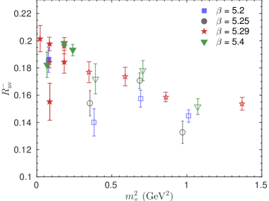
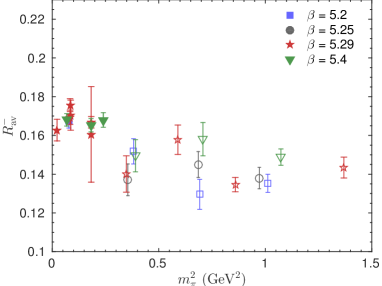
Figure 1: Bare results for $R_{\mathrm{av}}^{-}$ from this work (filled symbols) and from [5] (open symbols) for the two interpolators $J_{45}$ (left panel) and $J_{5}$ (right panel).

The bare data are renormalized using the nonperturbatively computed renormalization factors $\zeta_{11}$, $\zeta_{12}$, $\zeta_{22}$, after which the extrapolation to the physical pion mass, infinite volume, and eventually to the continuum has to be performed. The finite volume effects do not seem to be significant so we do not discuss them here. The finite lattice spacing effects for $\langle 1^{2}\rangle^{{\overline{\mathrm{MS}}}}$ and $a_{2}^{\overline{\mathrm{MS}}}$ are illustrated in Fig. 2. For the former, the results can very nicely be extrapolated to the continuum limit $a=0$, reproducing the expected result. For the latter, however, large statistical fluctuations do not allow for an extrapolation. Although our data may show a tendency for $a_{2}^{\overline{\mathrm{MS}}}$ (and $\langle\xi_{2}^{\overline{\mathrm{MS}}}\rangle$) decreasing in the continuum limit, we do not consider this evidence as sufficient. By this reason we choose to present our final results for finite lattice spacing leaving the continuum extrapolation for a future study.

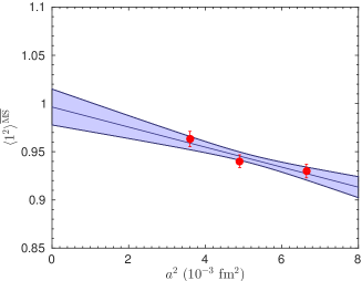
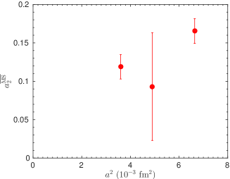
Figure 2: $\langle 1^{2}\rangle^{{\overline{\mathrm{MS}}}}$ [left panel] and $a_{2}^{\overline{\mathrm{MS}}}$ [right panel] as a function of the lattice spacing $a$ for ensembles with $m_{\pi}L\sim 3.4-3.8$ and $m_{\pi}\sim 280\,\mathrm{MeV}$. Only statistical errors are shown.

It is known [10] that $\langle\xi^{2}\rangle^{{\overline{\mathrm{MS}}}}$ and $a_{2}^{{\overline{\mathrm{MS}}}}$ do not contain chiral logarithms, at least to one-loop order. Therefore we assume a linear dependence on $m_{\pi}^{2}$ for the extrapolation in the pion mass to the physical value. Since the ensemble with the lightest pion in our simulations is already very close to the physical point, the chiral extrapolation should be reliable. As our lattice spacings do not vary that much, and a proper continuum extrapolation of $\langle\xi^{2}\rangle^{{\overline{\mathrm{MS}}}}$ and $a_{2}^{{\overline{\mathrm{MS}}}}$ cannot be attempted, we average the results from all lattice spacings but take into account only the data for the largest volume. The resulting extrapolations of $a_{2}^{{\overline{\mathrm{MS}}}}$ and $\langle\xi^{2}\rangle^{\overline{\mathrm{MS}}}$ to the physical pion mass are plotted in Fig. 3.

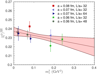
Figure 3: Extrapolation to the physical pion mass for $a_{2}^{\overline{\mathrm{MS}}}$ [left panel] and $\langle\xi^{2}\rangle^{\overline{\mathrm{MS}}}$ [right panel]. The open triangle represents the extrapolated value. Only statistical errors are shown.

5 Summary

In this work we extend the lattice study [5] of the second moment of the pion DA by making use of a larger set of lattices with different volumes, lattice spacings and pion masses down to $m_{\pi}\sim 150\,\mathrm{MeV}$ and implementing several technical improvements. We employ the variational approach with two and three interpolators (not discussed above) to improve the signal from the pion state. The renormalization of the lattice data is performed nonperturbatively utilizing a version of the RI’-SMOM scheme. For the first time we include a nonperturbative calculation of the renormalization factor corresponding to the mixing with total derivatives, which proves to have a significant effect. Our main result is

$$a_{2}=0.1364(154)(145)(?)$$ (28)

for the second Gegenbauer moment of the pion DA, and

$$\langle\xi^{2}\rangle=0.2361(41)(39)(?)\,.$$ (29)

They can be compared with the earlier lattice calculations

$$\langle\xi^{2}\rangle^{\overline{\mathrm{MS}}} =0.269(39)\,,\quad a_{2}^{\overline{\mathrm{MS}}}=0.201(114)\,,$$ [5]

$$\langle\xi^{2}\rangle^{\overline{\mathrm{MS}}} =0.28(1)(2)\,,\quad a_{2}^{\overline{\mathrm{MS}}}=0.233(29)(58)\,.$$ [6] (30)

All numbers refer to the scale $\mu=2\,\mathrm{GeV}$ in the ${\overline{\mathrm{MS}}}$ scheme. The first error in (28) and (29) combines the statistical uncertainty and the uncertainty of the chiral extrapolation. The second error is the estimated uncertainty contributed by the nonperturbative determination of the renormalization and mixing factors. Our lattice data are collected for the lattice spacing $a=0.06-0.08\,\mathrm{fm}$, and this range is not large enough to ensure a reliable continuum extrapolation. The corresponding remaining uncertainty is indicated as (?). It has to be addressed in a future study.

As a final remark, we note that the somewhat smaller value of $a_{2}^{\overline{\mathrm{MS}}}$ obtained in this work seems to be favored by the phenomenological studies of form factors in the framework of light-cone sum rules [11], see, e.g., Refs. [12, 13, 14, 15, 16]. Comparable numbers ($\langle\xi^{2}\rangle=0.25$, $a_{2}=0.15$) have also been obtained recently in the DSE approach in the calculation using DCSB-improved kernels [17].

- [1] V. L. Chernyak and A. R. Zhitnitsky, JETP Lett. 25, 510 (1977); Sov. J. Nucl. Phys. 31, 544 (1980).
- [2] A. V. Efremov and A. V. Radyushkin, Theor. Math. Phys. 42, 97 (1980) Phys. Lett. B 94, 245 (1980).
- [3] G. P. Lepage and S. J. Brodsky, Phys. Lett. B 87, 359 (1979); Phys. Rev. D 22, 2157 (1980).
- [4] V. M. Braun, S. Collins, M. Göckeler, P. Pérez-Rubio, A. Schäfer, R. W. Schiel and A. Sternbeck, Phys. Rev. D 92, no. 1, 014504 (2015).
- [5] V. M. Braun et al., Phys. Rev. D 74, 074501 (2006).
- [6] R. Arthur, P. A. Boyle, D. Brömmel, M. A. Donnellan, J. M. Flynn, A. Jüttner, T. D. Rae and C. T. C. Sachrajda, Phys. Rev. D 83, 074505 (2011).
- [7] M. Göckeler et al., Phys. Rev. D 82, 114511 (2010) [Erratum-ibid. D 86, 099903 (2012)].
- [8] J. A. Gracey, Eur. Phys. J. C 71, 1567 (2011).
- [9] J. A. Gracey, Phys. Rev. D 84, 016002 (2011).
- [10] J. W. Chen, H. M. Tsai and K. C. Weng, Phys. Rev. D 73, 054010 (2006).
- [11] I. I. Balitsky, V. M. Braun and A. V. Kolesnichenko, Sov. J. Nucl. Phys. 44, 1028 (1986); Nucl. Phys. B 312, 509 (1989).
- [12] S. S. Agaev, V. M. Braun, N. Offen and F. A. Porkert, Phys. Rev. D 83, 054020 (2011).
- [13] S. S. Agaev, V. M. Braun, N. Offen and F. A. Porkert, Phys. Rev. D 86, 077504 (2012).
- [14] P. Ball and R. Zwicky, Phys. Rev. D 71, 014015 (2005) [hep-ph/0406232].
- [15] G. Duplancic et al., JHEP 0804, 014 (2008).
- [16] A. Khodjamirian, T. Mannel, N. Offen and Y.-M. Wang, Phys. Rev. D 83, 094031 (2011).
- [17] L. Chang, I. C. Cloet, J. J. Cobos-Martinez, C. D. Roberts, S. M. Schmidt and P. C. Tandy, Phys. Rev. Lett. 110, no. 13, 132001 (2013).
- [18] R. G. Edwards et al. [SciDAC and LHPC and UKQCD Collaborations], Nucl. Phys. Proc. Suppl. 140, 832 (2005).
- [19] Y. Nakamura and H. Stüben, PoS LATTICE 2010, 040 (2010).
- [20] A. Nobile, PoS LATTICE 2010, 034 (2010).
- [21] M. Lüscher and S. Schaefer, http://cern.ch/luscher/openQCD (2012).