NLO K-factors for Single-Inclusive Leptoproduction of Hadrons

Abstract:

In these proceedings we discuss next-to-leading order (NLO) perturbative-QCD calculations of the cross section for the process $\ell N\rightarrow hX$. We briefly present the main features of the calculation and in particular analyze the role of quasi-real photons that enter the processes because the scattered lepton is not observed. We find that the NLO corrections are sizable for the spin-averaged cross section. In order to quantify this statement we present the K-factors of the cross sections for fixed target experiments HERMES, JLab12 and COMPASS.

1 Introduction

The process $\ell N\rightarrow hX$, i.e., the single inclusive production of a hadron at large transverse momentum in lepton-nucleon scattering, has attracted a lot of interest recently, both experimentally [1, 2, 3, 4] and theoretically [5, 6, 7, 8, 9, 10]. The reason for the interest in $\ell N\rightarrow hX$ comes from the study of single transverse-spin phenomena in hadronic scattering processes. It is well known that large single-spin asymmetries have been observed [11] for the process $pp^{\uparrow}\rightarrow hX$, where $p^{\uparrow}$ denotes a transversely polarized proton. To explain the large size of the asymmetries, and their persistence all the way from fixed-target to collider energies, has posed a major challenge to theory. Although a lot has been learned, it is fair to say that a fully satisfactory understanding has yet to be obtained. Measurements of corresponding asymmetries in the kinematically equivalent, but much simpler, processes $\ell N^{\uparrow}\rightarrow hX$, $\ell N^{\uparrow}\rightarrow\mathrm{jet}\,X$ have the promise to shed new light on the mechanisms for single-spin asymmetries in QCD. First fairly precise experimental data for $\ell N^{\uparrow}\rightarrow hX$ have recently been released by the HERMES [2, 3] and Jefferson Lab Hall A [4] collaborations.

We note that at first sight one might consider the related process $\ell N^{\uparrow}\rightarrow\ell^{\prime}X$ (which is just the standard inclusive deep-inelastic (DIS) process) to be equally suited for transverse-spin studies in lepton scattering. However, the analysis of the corresponding single-spin asymmetry is considerably more complex because higher order QED effects are required for the asymmetry to be non-vanishing [12, 13, 14, 15, 16]. In the same spirit as $\ell N^{\uparrow}\rightarrow hX$, also the processes $\vec{\ell}N^{\uparrow}\rightarrow hX$ [17] with longitudinal polarization of the lepton and $\ell N\rightarrow\Lambda^{\uparrow}X$ [18] with a transversely polarized $\Lambda$ hyperon have been considered in the literature recently.

The proven method for analyzing single-inclusive processes such as $pp\rightarrow hX$ or $\ell N\rightarrow hX$ at large transverse momentum rests on QCD perturbation theory and collinear factorization. For single-transverse-spin observables, this involves a twist-3 formalism in terms of three-parton correlation functions of the nucleon or the fragmentation process [19, 20, 21, 22, 23, 24, 25, 26, 27, 28]. Interestingly, the recent study [28] suggests that the twist-3 fragmentation effects could be the dominant source of the observed large transverse-spin asymmetries in $pp^{\uparrow}\rightarrow hX$.

The collinear twist-3 approach has been used recently to obtain predictions for the spin asymmetry in $\ell N^{\uparrow}\rightarrow hX$. In Ref. [7] a leading order (LO) twist-3 analysis has been presented in terms of parton correlation functions that were previously extracted from data for $pp^{\uparrow}\rightarrow hX$. The results obtained in this way fail to describe the HERMES data [2, 3] for the spin asymmetries in $\ell N^{\uparrow}\rightarrow hX$. A comparison of perturbative calculations to the corresponding JLab data [4] is not possible as the data are for hadrons with transverse momenta below 1 GeV.

In our view it is premature to draw any conclusions from these findings at LO. Given the kinematics (and the precision) of the present data, one may expect higher-order QCD corrections to the cross sections and the asymmetry to be important [7] for a meaningful comparison of data and theory. At least next-to-leading order (NLO) corrections should be included. We stress that the twist-3 formalism, although so far only developed to LO, offers a well-defined framework for a perturbative study of the transverse-spin asymmetry in $\ell N^{\uparrow}\rightarrow hX$.

In a recent paper [29], we took a first step toward an NLO calculation of the transverse-spin asymmetry for $\ell N^{\uparrow}\rightarrow hX$ by computing the NLO corrections to the spin-averaged cross section for the process, which constitutes the denominator of the spin asymmetry. In the following we will briefly present the main steps of the NLO calculation of Ref. [29]. Numerical predictions of the unpolarized cross-sections for several future and present-day experiments were presented as well in [29]. We found in [29] that the NLO corrections can become quite sizeable in particular for experiments at lower energies. It is illustrative to consider so-called K-factors, i.e. the ratio of the NLO-result divided by the LO-result for a certain observable. The K-factors quantify the size of the NLO-correction, and we will give numerical predictions for those K-factors in these proceedings.

2 NLO calculation

First, we give a brief review of the calculation presented in Ref. [29] of the spin-averged cross section of the process $\ell(l)+N(P)\rightarrow h(P_{h})+X$ up to NLO accuracy in pQCD. A large transverse momentum $P_{h\perp}\gg\Lambda_{\mathrm{QCD}}$ of the produced hadron sets a hard scale, so that perturbative methods may be used for treating the cross sections. It is useful to introduce the Mandelstam variables as $S=(P+l)^{2}$, $T=(P-P_{h})^{2}$ and $U=(l-P_{h})^{2}$. Furthermore, we label the energy of the detected hadron as $E_{h}$ and its three-momentum by $\vec{P}_{h}$.

In collinear leading-twist perturbative QCD the hadronic cross section is approximated by convolutions of hard partonic scattering cross sections and parton distribution/fragmentation functions. The momenta of the incoming parton, $k^{\mu}$, and of the fragmenting parton, $p^{\mu}$, which appear in the calculation of the partonic cross sections, are approximated as $k^{\mu}\simeq xP^{\mu}$ and $p^{\mu}\simeq P_{h}^{\mu}/z$, respectively. It is then convenient to work with the partonic Mandelstam variables

$$s=(k+l)^{2}=xS,\;\,t=(k-p)^{2}=\frac{x}{z}T,\;\,u=(l-p)^{2}=\frac{U}{z}\,.$$ (1)

The general form of the factorized cross section for the inclusive hadron production process then is

$$E_{h}\frac{d^{3}\sigma^{\ell N\rightarrow hX}}{d^{3}P_{h}} = \frac{1}{S}\sum_{i,f}\int_{0}^{1}\frac{dx}{x}\int_{0}^{1}\frac{dz}{z^{2}}\,f^{i/N}(x,\mu)D^{h/f}(z,\mu)\;\hat{\sigma}^{i\rightarrow f}(s,t,u,\mu)\;,$$ (2)

where $f^{i/N}(x,\mu)$ is the parton distribution function (PDF) for the incoming parton $i$ in the nucleon $N$ and $D^{h/f}(z,\mu)$ the corresponding fragmentation function (FF) for parton $f$ fragmenting into hadron $h$, both evaluated at a factorization scale $\mu$. In Eq. (2), $\hat{\sigma}^{i\rightarrow f}$ is the partonic cross section for the lepton-parton scattering process, $\ell+i\rightarrow f+x$, with $x$ an unobserved partonic final state. The sum in Eq. (2) runs over the different species of partons, quarks, gluons and antiquarks.

The partonic cross sections $\hat{\sigma}^{i\rightarrow f}$ in Eq. (2) can be calculated in QCD perturbation theory. One may write their expansion in the strong coupling as

$$\hat{\sigma}^{i\rightarrow f}\,=\,\hat{\sigma}^{i\rightarrow f}_{\mathrm{LO}}+\frac{\alpha_{s}}{\pi}\,\hat{\sigma}^{i\rightarrow f}_{\mathrm{NLO}}+{\cal O}(\alpha_{s}^{2})\,.$$ (3)

At lowest order (LO) only the tree-level process $\ell q\rightarrow q\ell$ shown in Fig. 1a contributes. The calculation of its cross section is straightforward. One finds

$$\hat{\sigma}_{\mathrm{LO}}^{q\rightarrow q}=2\alpha_{\mathrm{em}}^{2}e_{q}^{2}\;\frac{s^{2}+u^{2}}{t^{2}}\;\delta(s+t+u)\;,$$ (4)

where $\alpha_{\mathrm{em}}$ is the fine structure constant and $e_{q}$ is the quark’s fractional charge.

(a)

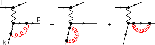
(b)

Figure 1: a) LO diagram for lepton-quark scattering. b) Virtual diagrams at NLO in Feynman gauge.

For a calculation of the hard partonic cross section to NLO accuracy it is convenient to rewrite the $x$- and $z$-integrals in Eq. (2) in terms of new variables $v=1+t/s$ and $w=-u/(s+t)$. Using (1), we have

$$x=\frac{1-v}{vw}\frac{U}{T}\,,\;\;z=\frac{-T}{(1-v)S}\,,$$ (5)

and Eq. (2) becomes

$$E_{h}\frac{d^{3}\sigma^{\ell N\rightarrow hX}}{d^{3}P_{h}} = \left(\frac{-U}{S^{2}}\right)\sum_{i,f}\int_{\frac{U}{T+U}}^{1+\frac{T}{S}}\frac{dv}{v(1-v)}\int_{\tfrac{1-v}{v}\tfrac{U}{T}}^{1}\frac{dw}{w^{2}}H^{if}(v,w)\;\hat{\sigma}^{i\rightarrow f}(v,w,\mu)\;,$$ (6)

where we have defined

$$H^{if}(v,w) \equiv \frac{f^{i/N}(x,\mu)}{x}\frac{D^{h/f}(z,\mu)}{z^{2}}\Bigg{|}_{x=\tfrac{1-v}{vw}\tfrac{U}{T},\,z=\tfrac{-T}{(1-v)S}}\,.$$ (7)

We note that the invariant mass of the unobserved recoiling partonic final state is given by $s+t+u=sv(1-w)$. The function $\delta(s+t+u)\propto\delta(1-w)$ in the LO cross section (4) expresses the fact that at LO the recoil consists of a single parton.

At the NLO level, the virtual contributions shown in Fig. 1b contribute through their interference with the Born diagram in Fig. 1a. The virtual contributions thus have Born kinematics and are proportional to $\delta(1-w)$. Since we are only interested in QCD virtual corrections, only the quark line is affected, and we may adopt the result directly from the corresponding calculation in Ref. [30] for the basic photon-quark scattering diagrams in DIS. This gives

$$\hat{\sigma}^{q\rightarrow q}_{\mathrm{NLO,vir}} = \frac{C_{F}\alpha_{s}(\mu)}{2\pi}\frac{\Gamma(1-\varepsilon)^{2}\Gamma(1+\varepsilon)}{\Gamma(1-2\varepsilon)}\left(\frac{4\pi\mu^{2}}{-t}\right)^{\varepsilon}\left(-\frac{2}{\varepsilon^{2}}-\frac{3}{\varepsilon}-8\right)\hat{\sigma}^{q\rightarrow q}_{\mathrm{LO},\varepsilon}\;,$$ (8)

where

$$\hat{\sigma}^{q\rightarrow q}_{\mathrm{LO},\varepsilon}=2\alpha_{\mathrm{em}}^{2}e_{q}^{2}\frac{1}{sv}\;\Bigg{(}\frac{1+v^{2}}{(1-v)^{2}}-\varepsilon\Bigg{)}\;\delta(1-w)\;.$$ (9)

is the Born cross section computed in $4-2\varepsilon$ dimensions. Furthermore, $C_{F}=(N_{c}^{2}-1)/2N_{c}$, with $N_{c}$ the number of colors.

The real diagrams in Figs. 2a, 2b, 2c have $2\rightarrow 3$ topology. To obtain the desired contribution to an inclusive-parton cross section we need to integrate over the phase space of the lepton and the “unobserved” parton in the final state. This can be done in $4-2\varepsilon$ dimensions using the standard techniques available in the literature [31, 32, 33].

The result for the real NLO contributions in $4-2\varepsilon$ dimensions, although well-defined, is rather lengthy and not presented at this point. The limit $\varepsilon\rightarrow 0$ has to be taken with care. In an expansion in $\varepsilon$ one finds a resulting $1/\varepsilon^{2}$-pole which constitutes itself in the $q\rightarrow q$ channel in Fig. 2a. This double pole cancels against the $1/\varepsilon^{2}$-pole of the virtual contribution in Eq. (8). This behaviour reflects the cancelation of infrared singularities in partonic observables.

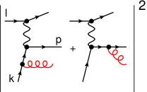
(a)

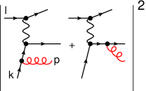
(b)

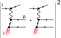
(c)

Figure 2: NLO real-emission diagrams. There are three partonic channels at NLO: (a) $q\rightarrow q$, (b) $q\rightarrow g$, (c) $g\rightarrow q$.

After the cancelation of infrared singularities between real and virtual contributions, the partonic cross sections still exhibit single poles $1/\varepsilon$ that reflect collinear singularities arising when an “observed” parton (either the incoming one, or the one that fragments) becomes collinear with the unobserved parton. The factorization theorem states that these poles may be absorbed into the parton distribution functions or into the fragmentation functions. This procedure may be formulated in terms of renormalized parton densities and fragmentation functions.

Even after this procedure, one type of collinear singularity remains. It is generated by a momentum configuration where the exchanged photon is collinear to the incoming lepton. The presence of this singularity is an artifact of neglecting the lepton’s mass.

One approach for dealing with the collinear lepton singularity is to introduce bare and renormalized QED parton distributions for the lepton $\--$ typically called Weizsäcker-Williams (WW) distributions [34, 35] $\--$ much in analogy with the renormalization procedure for the nucleon’s parton distributions. The only differences are that for leptons the partons are the lepton itself and the photon, and that we can safely compute their distributions in QED perturbation theory (cf. Ref. [29]).

The hard process involving an incoming lepton will always require two electromagnetic interactions and hence be of order $\alpha_{\mathrm{em}}^{2}$, as seen explicitly in Eq. (4). This is different for a hard process with an incoming photon such as $\gamma q\rightarrow qg$, which is of order $\alpha_{\mathrm{em}}\alpha_{s}$. This implies that at NLO in QCD (at order $\alpha_{\mathrm{em}}^{2}\alpha_{s}$) there will be contributions generated by the photon acting as a parton of the lepton and participating in the hard process. Such types of contributions are known as Weizsäcker-Williams contributions. In essence, in this situation the lepton merely serves as a source of real photons for those WW - contributions.

Since the Weizsäcker-Williams distribution is subject to ($\bar{\mathrm{MS}}$)-renormalization as well, the remaining collinear singularity that we encounter in the calculation of the real NLO contributions in Figs. 2a, 2b, 2c is canceled in this renormalization procedure. Eventually, one ends up with a well-defined NLO result in four dimensions.

One may adopt a second approach to deal with the collinear lepton-photon singularity. In principle one may perform a full calculation in which the lepton’s mass is kept finite. This is trivial for the virtual diagrams, since the QCD corrections do not affect the lepton line. However, inclusion of a lepton mass considerably complicates the phase space integrations for the real diagram. Nevertheless, it is possible to compute the relevant integrals using the results given in Ref. [32]. One may then expand the result in powers of the lepton mass and neglect terms suppressed by powers of $\mathcal{O}(m_{\ell})$. In this way, the “would-be” collinear singularity is regularized by the lepton mass and shows up as a term $\sim\ln(m_{\ell}^{2})$. Terms independent of $m_{\ell}$ are also kept.

One explicitly finds that the two approaches for treating the initial lepton are equivalent: The full result obtained using the WW contribution agrees with that for $m_{\ell}\neq 0$, as long as one only keeps the leading terms.

Next, we briefly present the structure of the final results for the full partonic cross sections in analytic form. Combining the cross section (6) for massless leptons with the Weizsäcker-Williams contribution we may write the full NLO cross section as

$$E_{h}\frac{d^{3}\sigma^{\ell N\rightarrow hX}}{d^{3}P_{h}} = \left(\frac{-U}{S^{2}}\right)\sum_{i,f}\int_{\frac{U}{T+U}}^{1+\frac{T}{S}}\frac{dv}{v(1-v)}\int_{\tfrac{1-v}{v}\tfrac{U}{T}}^{1}\frac{dw}{w^{2}}H^{if}(v,w)\;\left[\hat{\sigma}^{i\rightarrow f}_{\mathrm{LO}}(v)+\frac{\alpha_{s}(\mu)}{\pi}\,\hat{\sigma}^{i\rightarrow f}_{\mathrm{NLO}}(v,w,\mu)\right.$$ (10)

$$\hskip 85.35826pt+f^{\gamma/\ell}_{\mathrm{ren}}\left(\tfrac{1-v}{1-vw},\mu\right)\,\frac{\alpha_{s}(\mu)}{\pi}\,\hat{\sigma}_{\mathrm{LO}}^{\gamma i\rightarrow f}(v,w)\Bigg{]}\;,$$

where $H^{if}(v,w)$ has been defined in Eq. (7). The LO contribution, present only for the channel $q\rightarrow q$ with an incoming quark that also fragments, was already given in (4). For the NLO term in this channel we find

$$\hat{\sigma}_{\mathrm{NLO}}^{q\rightarrow q}(v,w,\mu) = \frac{\alpha_{\mathrm{em}}^{2}e_{q}^{2}C_{F}}{svw}\Bigg{[}A_{0}^{q\rightarrow q}\,\delta(1-w)+A_{1}^{q\rightarrow q}\left(\frac{\ln(1-w)}{1-w}\right)_{+}+\frac{1}{(1-w)_{+}}\Bigg{\{}B_{1}^{q\rightarrow q}\ln\left(\frac{1-v}{v(1-v(1-w))}\right)$$ (11)

$$+ B_{2}^{q\rightarrow q}\ln(1-v(1-w))+B_{3}^{q\rightarrow q}\ln\left(\frac{sv^{2}}{\mu^{2}}\right)\Bigg{\}}+C_{1}^{q\rightarrow q}\ln(v(1-w))+C_{2}^{q\rightarrow q}\ln\left(\frac{(1-v)w}{1-vw}\right)$$

$$+ C_{3}^{q\rightarrow q}\ln\left(\frac{1-v}{(1-vw)(1-v(1-w))}\right)+C_{4}^{q\rightarrow q}\ln\left(\frac{s}{\mu^{2}}\right)+C_{5}^{q\rightarrow q}\Bigg{]}\,,$$

where the coefficients $A_{i}^{q\rightarrow q}$, $B_{i}^{q\rightarrow q}$, $C^{q\rightarrow q}_{i}$ are functions of $v$ and $w$ and their explicit form may be found in Ref. [29]. The channels $q\rightarrow g$ and $g\rightarrow q$ have simpler expressions:

$$\hat{\sigma}_{\mathrm{NLO}}^{q\rightarrow g}(v,w,\mu) = \frac{\alpha_{\mathrm{em}}^{2}e_{q}^{2}C_{F}}{svw}\Bigg{[}C_{1}^{q\rightarrow g}\ln(1-v(1-w))+C_{2}^{q\rightarrow g}\ln\left(\frac{1-v}{(1-vw)(1-v(1-w))}\right)$$ (12)

$$\hskip 85.35826pt+C_{3}^{q\rightarrow g}\ln\left(\frac{v(1-w)s}{\mu^{2}}\right)+C_{4}^{q\rightarrow g}\Bigg{]}\,,$$

$$\hat{\sigma}_{\mathrm{NLO}}^{g\rightarrow q}(v,w,\mu) = \frac{\alpha_{\mathrm{em}}^{2}e_{q}^{2}T_{R}}{svw}\Bigg{[}C_{1}^{g\rightarrow q}\ln\left(\frac{(1-v)w}{1-vw}\right)+C_{2}^{g\rightarrow q}\ln\left(\frac{v(1-w)s}{\mu^{2}}\right)+C_{3}^{g\rightarrow q}\Bigg{]}\,.$$ (13)

The coefficients $C^{q\rightarrow g}_{i}$ and $C^{g\rightarrow q}_{i}$ are again given in Ref. [29]. The partonic cross sections $\hat{\sigma}_{\mathrm{LO}}^{\gamma q\rightarrow q}$, $\hat{\sigma}_{\mathrm{LO}}^{\gamma q\rightarrow g}$, $\hat{\sigma}_{\mathrm{LO}}^{\gamma g\rightarrow q}$ represent the Weizsäcker-Williams contributions in Eq. (10) for the relevant channels and we again refer the reader to Ref. [29] for their explicit form.

3 K-factors

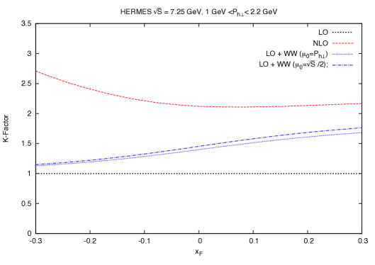
Figure 3: K-factor (at a scale $\mu=P_{h\perp}$) for the HERMES experiment plotted vs. the Feynman variable $x_{F}$ and a binned transverse momentum $P_{h\perp}$.

In Ref. [29] we utilized Eq. (10) in order to give numerical predictions for the spin-averaged cross section of the process $\ell+N\rightarrow h+X$ at fixed target experiments (Jefferson Lab, HERMES, COMPASS) and a collider experiment (EIC). We investigated differential cross sections depending on the longitudinal momentum component of the produced hadron (represented by a Feynman variable $x_{F}$ or pseudorapidity $\eta$) at a fixed transverse momentum $P_{h\perp}$, or vice versa. We have found particularly large NLO - corrections at low center-of-mass energies of the colliding lepton and nucleon, in particular at JLab and HERMES energies. Although potentially scale dependent, the so-called K-factor is an illustrative quantity to represent the magnitude of the NLO - corrections. It is defined as

$$K_{\mathrm{NLO}}=\frac{\sigma_{\mathrm{NLO}}}{\sigma_{\mathrm{LO}}}.$$ (14)

In the following we use the numerical results of Ref. [29] as input for the K-factors. In Fig. 3 we plot the K-factor for $\pi^{+}$-production at HERMES at $\sqrt{S}=7.25$ GeV. It shows the K-factor as a function of the Feynman variable $x_{F}$ in a bin $1\;\mathrm{GeV}<P_{h\perp}<2.2\;\mathrm{GeV}$. We also examine the situation where dominance of the Weizsäcker-Williams contribution is assumed and the NLO correction caused by $\hat{\sigma}^{i\rightarrow f}_{\mathrm{NLO}}$ is assumed to be negligible (cf. Ref. [29]), and plot the corresponding K-factors for two scales $\mu_{0}=P_{h\perp}$ and $\mu_{0}=\sqrt{S}/2$ in Fig. 3 ($\mu_{0}$ indicates a spurious scale in the separation of WW - contributions and partonic NLO - contributions, see Ref. [29]). However, Fig. 3 as well as Figs. 4 and 5 indicates that the LO term plus the WW contribution alone in Eq. (10) is not a good approximation for the full NLO result. We also note that we obtain K-factors of similar size ($\sim 2.5$) in a plot vs. the transverse hadron momentum $P_{h\perp}$.

In Fig. 4 we present our predictions for the K-factor as a function of $x_{F}$ for $\ell\;{}^{3}{\mathrm{He}}\rightarrow\pi^{+}X$ in 12 GeV scattering at the Jefferson Lab where we have assumed a fixed transverse momentum $P_{h\perp}=1.5\;\mathrm{GeV}$. We observe in Fig. 4 that the NLO corrections are even larger compared to Fig. 3 with a K-factor of about $\sim 2.5-3.5$. The $P_{h\perp}$-dependence (not shown here) displays a similar behaviour.

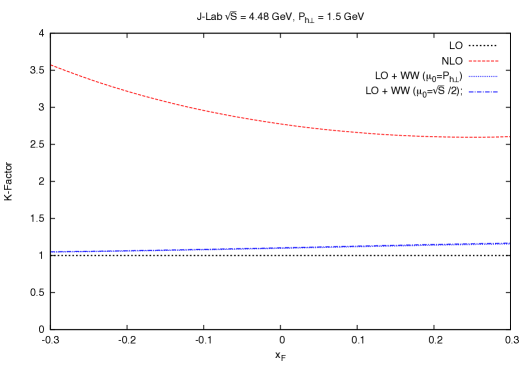
Figure 4: K-factor (at a scale $\mu=P_{h\perp}$) for the 12 GeV upgrade at Jefferson Lab plotted vs. $x_{F}$ and a fixed transverse momentum $P_{h\perp}$.

The result of our NLO K-factors for COMPASS kinematics is shown in Figs. 5. COMPASS uses a muon beam with energy 160 GeV, resulting in $\sqrt{S}=17.4$ GeV. Following the choice made by COMPASS, we use here the c.m.s. pseudorapidity $\eta$ of the produced hadron rather than its Feynman-$x_{F}$. Pseudorapidity is counted as positive in the forward direction of the incident muon. The COMPASS spectrometer roughly covers the region $-0.1<\eta<2.38$. From the $\eta$ dependence shown in Fig. 5 for a fixed transverse momentum $P_{h\perp}=2\;\mathrm{GeV}$ we observe that the NLO K-factors are significant but not as large as for HERMES and JLab. Their size is about $\sim 1.2-1.4$. Strikingly, the Weizsäcker-Williams contribution is very small here, even for the choice $\mu_{0}=\sqrt{S}/2$. This may be understood from the fact that the muon mass is about 200 times larger than the electron mass.

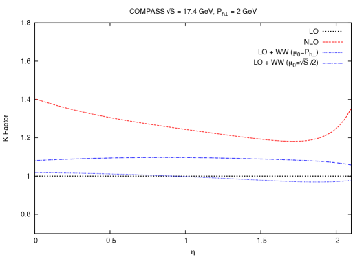
Figure 5: K-factor (at a scale $\mu=P_{h\perp}$) for the COMPASS experiment plotted vs. the pseudorapidity $\eta$ and a fixed transverse momentum $P_{h\perp}$.

4 Conclusions

We have described the next-to-leading order calculations of Ref. [29] of the partonic cross sections for the process $\ell N\rightarrow hX$ for which the scattered lepton in the final state is not detected. In particular we have discussed the situation where the exchanged photon is radiated collinearly to the incoming lepton. We have dealt with this situation in two ways. We have first set the mass to zero and have regularized the ensuing collinear singularity in dimensional regularization and then subtracted it by introducing a Weizsäcker-Williams type photon distribution in the lepton. In the second approach, we have kept the lepton mass in the calculation directly, expanding all phase space integrals in such a way that the leading mass dependence is obtained. Both approaches give the same result.

We have presented phenomenological NLO predictions for three experimental setups for the fixed-target experiments at HERMES, JLab12 and COMPASS in terms of NLO K-factors, a very illustrative quantity to display the magnitude of NLO-corrections. We have found that the K-factors are particularly large for the low energy experiments at JLab12 ($\sqrt{S}=4.48\,\mathrm{GeV}$) and HERMES ($\sqrt{S}=7.25\,\mathrm{GeV}$) where we predict K-factors from $2.5$ up to $3.5$. This behaviour has to be attributed to the fact that for those small energies the plus distribution terms in Eq. (11) are large, especially at negative $x_{F}$ or rapidity. For larger energies at COMPASS ($\sqrt{S}=17.4\,\mathrm{GeV}$) the K-factor is $1.2-1.4$. Hence, it is significant but well-behaved.

Because of the large K-factors at HERMES and Jefferson Lab one may wonder whether the perturbative expansion is under control. In particular when analyzing the data for a transversely polarized target [2, 3, 4], one should take care as NLO corrections for transverse spin polarization may be large as well. In fact, we argue that the unpolarized cross section should be measured simultaneously to polarized observables for those experiments in order to ensure that perturbative QCD works for the process $\ell+N\rightarrow h+X$ at lower c.m.-energies.

References

- [1] P. L. Anthony et al. [E155 Collaboration], Phys. Lett. B 458, 536 (1999) [hep-ph/9902412].
- [2] A. Airapetian et al. [HERMES Collaboration], Phys. Lett. B 728, 183 (2014) [arXiv:1310.5070 [hep-ex]].
- [3] C. Van Hulse [HERMES Collaboration], EPJ Web Conf. 85, 02020 (2015).
- [4] K. Allada et al. [Jefferson Lab Hall A Collaboration], Phys. Rev. C 89, 042201 (2014) [arXiv:1311.1866 [nucl-ex]].
- [5] Y. Koike, AIP Conf. Proc. 675, 449 (2003) [hep-ph/0210396]; Nucl. Phys. A 721, 364 (2003) [hep-ph/0211400];
- [6] Z. B. Kang, A. Metz, J. W. Qiu and J. Zhou, Phys. Rev. D 84, 034046 (2011) [arXiv:1106.3514 [hep-ph]].
- [7] L. Gamberg, Z. B. Kang, A. Metz, D. Pitonyak and A. Prokudin, Phys. Rev. D 90, 074012 (2014) [arXiv:1407.5078 [hep-ph]].
- [8] M. Anselmino, M. Boglione, J. Hansson and F. Murgia, Eur. Phys. J. C 13, 519 (2000) [hep-ph/9906418].
- [9] M. Anselmino, M. Boglione, U. D’Alesio, S. Melis, F. Murgia and A. Prokudin, Phys. Rev. D 81, 034007 (2010) [arXiv:0911.1744 [hep-ph]].
- [10] M. Anselmino, M. Boglione, U. D’Alesio, S. Melis, F. Murgia and A. Prokudin, Phys. Rev. D 89, 114026 (2014) [arXiv:1404.6465 [hep-ph]].
- [11] For review, see: C. A. Aidala, S. D. Bass, D. Hasch and G. K. Mallot, Rev. Mod. Phys. 85, 655 (2013) [arXiv:1209.2803 [hep-ph]].
- [12] N. Christ and T. D. Lee, Phys. Rev. 143, 1310 (1966).
- [13] A. Metz, M. Schlegel and K. Goeke, Phys. Lett. B 643, 319 (2006) [hep-ph/0610112].
- [14] A. Afanasev, M. Strikman and C. Weiss, Phys. Rev. D 77, 014028 (2008) [arXiv:0709.0901 [hep-ph]].
- [15] A. Metz, D. Pitonyak, A. Schafer, M. Schlegel, W. Vogelsang and J. Zhou, Phys. Rev. D 86, 094039 (2012) [arXiv:1209.3138 [hep-ph]].
- [16] M. Schlegel, Phys. Rev. D 87, 034006 (2013) [arXiv:1211.3579 [hep-ph]].
- [17] K. Kanazawa, A. Metz, D. Pitonyak and M. Schlegel, Phys. Lett. B 742, 340 (2015) [arXiv:1411.6459 [hep-ph]].
- [18] K. Kanazawa, A. Metz, D. Pitonyak and M. Schlegel, Phys. Lett. B 744, 385 (2015) [arXiv:1503.02003 [hep-ph]].
- [19] J. w. Qiu and G. F. Sterman, Phys. Rev. Lett. 67, 2264 (1991); Nucl. Phys. B 378, 52 (1992).
- [20] Y. Kanazawa and Y. Koike, Phys. Lett. B 478, 121 (2000) [hep-ph/0001021].
- [21] C. Kouvaris, J. W. Qiu, W. Vogelsang and F. Yuan, Phys. Rev. D 74, 114013 (2006) [hep-ph/0609238].
- [22] Z. B. Kang, F. Yuan and J. Zhou, Phys. Lett. B 691, 243 (2010) [arXiv:1002.0399 [hep-ph]].
- [23] K. Kanazawa and Y. Koike, Phys. Rev. D 83, 114024 (2011) [arXiv:1104.0117 [hep-ph]].
- [24] H. Beppu, K. Kanazawa, Y. Koike and S. Yoshida, Phys. Rev. D 89, 034029 (2014) [arXiv:1312.6862 [hep-ph]].
- [25] A. Metz and D. Pitonyak, Phys. Lett. B 723, 365 (2013) [arXiv:1212.5037 [hep-ph]].
- [26] F. Yuan and J. Zhou, Phys. Rev. Lett. 103, 052001 (2009) [arXiv:0903.4680 [hep-ph]].
- [27] K. Kanazawa and Y. Koike, Phys. Rev. D 88, 074022 (2013) [arXiv:1309.1215 [hep-ph]].
- [28] K. Kanazawa, Y. Koike, A. Metz and D. Pitonyak, Phys. Rev. D 89, 111501 (2014) [arXiv:1404.1033 [hep-ph]].
- [29] P. Hinderer, M. Schlegel and W. Vogelsang, Phys. Rev. D 92, 014001 (2015) [arXiv:1505.06415 [hep-ph]].
- [30] G. Altarelli, R. K. Ellis and G. Martinelli, Nucl. Phys. B 157, 461 (1979).
- [31] W. L. van Neerven, Nucl. Phys. B 268, 453 (1986).
- [32] W. Beenakker, H. Kuijf, W. L. van Neerven and J. Smith, Phys. Rev. D 40, 54 (1989).
- [33] L. E. Gordon and W. Vogelsang, Phys. Rev. D 48, 3136 (1993).
- [34] C. F. von Weizsäcker, Z. Phys. 88, 612 (1934).
- [35] E. J. Williams, Phys. Rev. 45, 729 (1934).