Optimal Temporal Patterns for Dynamical Cellular Signaling

Abstract

Cells use temporal dynamical patterns to transmit information via signaling pathways. As optimality with respect to the environment plays a fundamental role in biological systems, organisms have evolved optimal ways to transmit information. Here, we use optimal control theory to obtain the dynamical signal patterns for the optimal transmission of information, in terms of efficiency (low energy) and reliability (low uncertainty). Adopting an activation-deactivation decoding network, we reproduce several dynamical patterns found in actual signals, such as steep, gradual, and overshooting dynamics. Notably, when minimizing the energy of the input signal, the optimal signals exhibit overshooting, which is a biphasic pattern with transient and steady phases; this pattern is prevalent in actual dynamical patterns. We also identify conditions in which these three patterns (steep, gradual, and overshooting) confer advantages. Our study shows that cellular signal transduction is governed by the principle of minimizing free energy dissipation and uncertainty; these constraints serve as selective pressures when designing dynamical signaling patterns.

Department of Information and Communication Engineering, Graduate School of Information Science and Technology, The University of Tokyo, Tokyo 113-8656, Japan

1 Introduction

Cells transmit information through signal transduction and transcription networks [1, 2]. Recent studies have revealed that, along with the identity and static concentration of molecules, cells also encode information into dynamical patterns [3, 4, 5, 6, 7, 8, 9]. Examples of dynamical patterns include extracellular signal-regulated kinase (ERK), the yeast transcription factor Msn2, the transcription factor NF-$\kappa$B, a protein kinase AKT, and calcium signaling. Many studies have used nonlinear and stochastic approaches to investigate the properties of dynamical cellular information processing [10, 11, 12, 13, 14, 15, 16, 17]. Because signal transduction plays central and crucial roles in the survival of cells, the time course of dynamical patterns is expected to be highly optimized so that cells can efficiently and accurately transmit information. Although the advantages of dynamical signals over static ones have been extensively studied [18, 8], there has been little investigation into determining which dynamical signals are the best. We assume that two principles that are prevalent in many biological systems govern the optimality of signal patterns: energetic efficiency (low energy) and reliability (low uncertainty). Biological systems are often characterized by low energy consumption. For instance, neuronal systems are known to function with remarkably low energy consumption. Specifically, in neurons, information processing capability is bounded by the amount of energy consumption and it is reported that the energy consumption of the brain has limited its size ([19, 20] and references therein). Biochemical networks process information for a variety of purposes, and higher specificity, lower variation, and larger signal amplification demand more energy consumption [21]. These facts induce us to think that the energetic cost also plays important roles in information transmission of the dynamical signal transduction. A major cause of interference with reliability is molecular noise, which degrades the quality of transmitted information. Despite the stochastic nature of cellular processes, organisms have acquired several mechanisms to resist or to take advantage of noise in order to enhance biological functionalities [22]. As these two principles are of significance, the dynamical transmission of information has evolved in such a way that it optimally satisfies these principles. We divide the dynamical signal transduction into two parts: encoding of extracellular stimuli into intracellular dynamical patterns, and decoding of the dynamical patterns into the response (in the present manuscript, the response corresponds to the concentration of output molecular species) (Fig. 1(a)). By viewing the dynamical signal as an input, the decoding network as the system to be controlled, and the output concentration as an output (Fig. 1(a)), we use optimal control theory [23, 24] to determine the signal dynamics that optimize energy efficiency and the reliability of transmitted information. We quantify the energetic cost by free energy dissipation when generating temporal dynamical patterns and the uncertainty by variance of output molecular species concentration. To decode the dynamical signals, we adopt an activation-deactivation network (Fig. 1(b)), which is a motif commonly used in biochemical networks. We optimize the dynamical patterns, i.e. the input. Decoders (decoding networks) may also coevolve to maximally reading out information from signals, but in this paper, we focus on optimizing the input. No matter how precisely the decoder is able to read dynamical signals, it is impossible to totally eliminate the uncertainty due to the inherent stochasticity. Therefore, there is a lower bound on the uncertainty and the bound is determined by input.

From our calculations, we identify three basic patterns for the signals: steep (Fig. 2(a)), gradual (Fig. 2(b)), and overshooting (Fig. 2(c)). We show that the steep pattern minimizes the energy, whereas the gradual pattern minimizes the uncertainty. Intriguingly, when minimizing the energy of a dynamical pattern while achieving a higher output concentration, overshooting is the optimal pattern; this pattern can often be seen in real processes. We identify the conditions in which these three patterns (steep, gradual, and overshooting) confer advantages. We note that these patterns are prevalent in signal transduction, and our calculations show that minimizing the energetic cost and uncertainty plays important roles in the evolutionary design of dynamical signaling patterns.

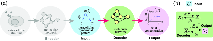
Figure 1: Overview of dynamical signal transduction. (a) An extracellular stimulus is encoded into an intracellular dynamical pattern. The decoder reads the dynamical pattern and outputs the result as the final concentration. This study focuses on the latter process (colored flow). The intracellular dynamical pattern $u(t)$ and the final concentration $x_{i_{\mathrm{out}}}(T)$ correspond to input and output, respectively, and we optimize the dynamical pattern. (b) Two-molecule decoding network (the two-stage model), which reports the result as $X_{2}$. $\overline{X}_{i}$ and $X_{i}$ ($i=1,2$) denote the inactive and active molecules, respectively.

2 Methods

2.1 Model

Dynamical signal transduction is typically separated into two parts [7]: encoding of extracellular stimuli into intracellular dynamical patterns, and decoding of the dynamical patterns into the response (Fig. 1(a)); our study focuses on the latter process, and dynamical signals are optimized for readout by a particular decoder, where the optimization criteria are to minimize the energy consumed by signal generation and to minimize the uncertainty of the readout.

In cells, dynamical signals are decoded by molecular networks. We consider a molecular network consisting of $N$ molecular species $X_{1},X_{2},...,X_{N}$ and we define $x_{i}$ as the concentration of $X_{i}$. The input signal is carried by a molecular species $U$, whose concentration $u(t)$ follows a dynamic pattern, and its onset is $t=0$. In our analysis, we use optimal control theory to optimize the temporal pattern of $u(t)$. Let the $i_{\mathrm{out}}$th molecular species $X_{i_{\mathrm{out}}}$ be the output of the network. The network reads the information from the input $u(t)$ (i.e., intracellular dynamical signal) and outputs the result as the concentration of $X_{i_{\mathrm{out}}}$ at time $T$ ($T>0$) (Fig. 1(a)), i.e., $x_{i_{\mathrm{out}}}(T)$ carries information about the input signal.

Consider the evolutionary design of the dynamical signal $u(t)$ that attains the desired concentration of an output molecule $X_{i_{\mathrm{out}}}$ at $t=T$. Although there might be many possible dynamics for $u(t)$ ($0\leq t\leq T$) that result in the desired output concentration, the most biologically preferable ones are selected. We can expect that the signals with lower energetic cost will be selected. In addition, biochemical reactions are subject to noise, due to the smallness of the cells. The noise degrades the information, and hence transmission with lower uncertainty is desirable. Considering the energy of the input and the uncertainty of the concentration of the output molecule, we wish to find a signal $u(t)$ that minimizes a performance index $R$, defined as

$$R=\gamma_{i_{\mathrm{out}}}(T)+w\Pi,$$ (1)

where $\gamma_{i}(t)=\left\langle\left(x_{i}(t)-\mu_{i}(t)\right)^{2}\right\rangle$ is the variance of the concentration of the $i$th molecule at time $t$ [$\mu_{i}(t)=\left\langle x_{i}(t)\right\rangle$ is the mean] which quantifies the uncertainty, $\Pi$ is the energetic cost of the signal $u(t)$, and $w$ is a weight parameter in the range $0<w<\infty$, which represents the importance of the energy for the performance index. As denoted, the output $X_{i_{\mathrm{out}}}$ has the target concentration at time $t=T$. Therefore, the mean concentration of the output $X_{i_{\mathrm{out}}}$, which we denote as $\mu_{i_{\mathrm{out}}}(t)$, must attain the predefined target concentration $\mu_{i_{\mathrm{out}}}^{\mathrm{trg}}$ (“trg” is short for “target”) at time $t=T$, i.e.,

$$\mu_{i_{\mathrm{out}}}(T)=\mu_{i_{\mathrm{out}}}^{\mathrm{trg}}$$ (2)

is a boundary condition.

2.2 Quantification of uncertainty

We quantify the uncertainty as the variance of the output molecular species concentration $\gamma_{i_{\mathrm{out}}}(T)$; the derivation is shown below. The dynamics of molecular networks, which decode $u(t)$ and output the result, can be generally captured by the following rate equation:

$$\dot{x}_{i}(t)=\sum_{\ell=1}^{N_{r}}s_{i\ell}v_{\ell}(\boldsymbol{x},u),$$

where $\boldsymbol{x}=(x_{1},x_{2},...,x_{N})$, $\{s_{i\ell}\}=\boldsymbol{S}$ is a stoichiometry matrix, $v_{\ell}(\boldsymbol{x},u)$ is the reaction velocity of the $\ell$th reaction, and $N_{r}$ is the number of reactions. Due to the smallness of the cells, chemical reactions are subject to stochasticity. We describe the noisy dynamics by the Fokker–Planck equation (FPE) [25, 26]:

$$\frac{\partial}{\partial t}P(\boldsymbol{x};t)=-\sum_{i}\frac{\partial}{\partial x_{i}}\sum_{\ell}s_{i\ell}v_{\ell}(\boldsymbol{x},u)P(\boldsymbol{x};t)+Q\sum_{i,j}\frac{\partial^{2}}{\partial x_{i}\partial x_{j}}\sum_{\ell}s_{i\ell}s_{j\ell}v_{\ell}(\boldsymbol{x},u)P(\boldsymbol{x};t),$$ (3)

where $P(\boldsymbol{x};t)$ is the probability density of $\boldsymbol{x}$ at time $t$, and $Q$ is the noise intensity related to the volume $V$ via $Q=(2V)^{-1}$. Optimal control theory and related variational methods have been employed by many researchers [27, 28, 29, 30, 31]. Although stochastic optimal control theory has been applied in biological contexts [31], it is difficult to apply it to multivariate models. Instead, we describe the dynamics by using the time evolution of moments derived from Eq. (3) [32, 33]. For general nonlinear models, the naive calculation of moment equations results in an infinite hierarchy of differential equations. Because our adopted models are linear with respect to $\boldsymbol{x}$ (cf. Eqs. (15) and (16)), we can obtain closed differential equations (see the supplementary material). For moments of up to the second order [mean $\mu_{i}(t)$, variance $\gamma_{i}(t)$, and covariance $\rho_{ij}=\left\langle\left(x_{i}-\mu_{i}\right)\left(x_{j}-\mu_{j}\right)\right\rangle$], we have the following moment equation with respect to $\boldsymbol{z}=(\mu_{1},...,\mu_{n},\gamma_{1},...,\gamma_{n},\rho_{12},\rho_{23},...,\rho_{1n})$:

$$\dot{z}_{i}(t)=h_{i}(\boldsymbol{z},u),$$ (4)

where $h_{i}(\boldsymbol{z},u)$ is right-hand side of the moment equation and the dimensionality of $\boldsymbol{z}$ is $M=N(N+3)/2$. With the moment equation (4), we can reduce the stochastic optimal control problem to a deterministic one.

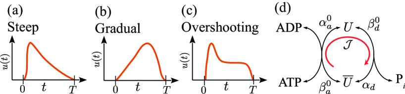
Figure 2: (a)–(c) Dynamical signal $u(t)$ ($0\leq t\leq T$) as a function of $t$ for the three typical patterns: (a) steep, (b) gradual, and (c) overshooting. (d) Activation-deactivation of signaling molecule $U$. Inactive molecule $\overline{U}$ is activated to become active molecule $U$, which is mediated by phosphorylation, and deactivation is mediated by dephosphorylation. Net flux $\mathcal{J}$ occurs in the clockwise direction (shown by an arrow).

2.3 Quantification of energetic cost

We next define the energetic cost of a signal ($\Pi$ in Eq. (1)) as the free energy dissipated by controlling the concentration $u(t)$ such that it follows the desired temporal dynamics. We derive the energetic cost of the signal $U$ with a simple biochemical model after Ref. [34, 35, 36]. We assume that input molecular species $U$ is activated from $\overline{U}$ and undergoes the following reaction:

$$\overline{U}\rightleftharpoons U.$$ (5)

Note that the total concentration $u^{\mathrm{tot}}=u+\overline{u}$ does not change with time, where $u$ and $\overline{u}$ are the concentrations of $U$ and $\overline{U}$, respectively. In general, the deactivation reaction is not the reverse of activation. Therefore, when considering the energetic cost of generating $U$, we have to handle activation and deactivation separately. Activation is typically mediated by phosphorylation, where $\overline{U}$ is activated by a kinase through the transfer of phosphate from ATP. The deactivation is mediated by dephosphorylation, in which a phosphatase transfers inorganic phosphate ($\mathrm{P}_{i}$) to the solution. These reactions are written as

$$\overline{U}+\mathrm{ATP}\xrightleftharpoons[\beta_{a}^{0}]{\alpha_{a}^{0}}U+\mathrm{ADP},\hskip 10.00002ptU\xrightleftharpoons[\beta_{d}^{0}]{\alpha_{d}}\overline{U}+\mathrm{P}_{i},$$ (6)

where $\alpha_{a}^{0}$, $\beta_{a}^{0}$, $\alpha_{d}$, and $\beta_{d}^{0}$ are reaction rates. When these parameters are held constant and the system is closed, the system relaxes to an equilibrium state. Let $c_{T}$, $c_{D}$, and $c_{P}$ be the concentrations of ATP, ADP, and $\mathrm{P}_{i}$, respectively. In the natural cellular environment where the system is open, $c_{T}$, $c_{D}$, and $c_{P}$ can be regarded as constant, due to external agents [35], which we denote as $c_{T}^{0}$, $c_{D}^{0}$, and $c_{P}^{0}$, respectively. Therefore the system relaxes to a nonequilibrium steady state (NESS). The steady-state concentration of $U$ is

$$u^{\mathrm{ss}}=\frac{u^{\mathrm{tot}}\left(\beta_{d}+\alpha_{a}\right)}{\beta_{a}+\beta_{d}+\alpha_{a}+\alpha_{d}},$$ (7)

where $\beta_{a}=\beta_{a}^{0}c_{D}^{0}$, $\alpha_{a}=\alpha_{a}^{0}c_{T}^{0}$, and $\beta_{d}=\beta_{d}^{0}c_{P}^{0}$. At the steady state, the net flux (clockwise direction in Fig. 2(d)) is $\mathcal{J}^{\mathrm{ss}}=u^{\mathrm{tot}}\left(\alpha_{a}\alpha_{d}-\beta_{a}\beta_{d}\right)/\left(\beta_{a}+\beta_{d}+\alpha_{a}+\alpha_{d}\right)$. The free energy dissipated during one cycle (i.e., $\overline{U}\rightarrow U\rightarrow\overline{U}$ in the clockwise direction in Fig. 2(d)) is $\Delta\phi=k_{B}\mathcal{T}\ln\left\{\beta_{a}\beta_{d}/\left(\alpha_{a}\alpha_{d}\right)\right\}$, where $k_{B}$ is the Boltzmann constant and $\mathcal{T}$ is the temperature (see the supplementary material). Therefore the instantaneous free-energy dissipation (i.e., power) is

$$\mathcal{P}=-\mathcal{J}^{\mathrm{ss}}\Delta\phi=\frac{k_{B}\mathcal{T}u^{\mathrm{tot}}\left(\alpha_{a}\alpha_{d}-\beta_{a}\beta_{d}\right)}{\beta_{a}+\beta_{d}+\alpha_{a}+\alpha_{d}}\ln\left(\frac{\alpha_{a}\alpha_{d}}{\beta_{a}\beta_{d}}\right).$$ (8)

Equation (8) quantifies the cost of the activation-deactivation of $U$. Next, in order to yield the dynamics of $U$, we assume that kinase activity is controlled by an upstream molecular species and thus $\alpha_{a}$ varies temporally. We assume that the relaxation of Eq. (6) is very fast [i.e., $1/(\beta_{a}+\beta_{d}+\alpha_{a}+\alpha_{d})$ is very small] so that the concentration $u$ is well approximated by $u^{\mathrm{ss}}$ (Eq. (7)) even for the case of a time-varying $\alpha_{a}$. From Eq. (7), $\alpha_{a}$ can be represented as a function of $u$:

$$\alpha_{a}=\frac{u}{u^{\mathrm{tot}}-u}\left(\alpha_{d}+\beta_{a}\right)-\beta_{d}.$$ (9)

From the condition $\alpha_{a}>0$, the minimum of $u$ is $u^{\min}=\beta_{d}u^{\mathrm{tot}}/\left(\beta_{a}+\beta_{d}+\alpha_{d}\right)$. For this dynamic case, the instantaneous free energy dissipation is given as a function of $u$ which is Eq. (8) along with Eq. (9). The molecular species upstream from $U$ also consumes energy; however, signal transduction generally amplifies the external stimuli, and so the concentration of the upstream molecular species is less than the concentration of $U$ [37, 38]. Furthermore, we assume that the concentration of the molecular species downstream from $U$ is also less than that of $U$ [37, 38]. Indeed, in the ERK pathway, the concentration of ERK is higher than that of its downstream molecular species (that is, the energetic cost of decoding $U$ is smaller than the cost of generating it). Therefore, we assume that the energetic cost of generating $U$ (i.e., Eq. (8)) dominates the overall energetic cost. The free energy dissipated during $0\leq t\leq T$ is

$$\Pi=\int_{0}^{T}\mathcal{P}dt.$$ (10)

Because it is difficult to use the exact representation of $\Pi$ in the optimal control calculation, we approximate $\mathcal{P}$ with a simpler expression: $\mathcal{P}=0$ at a zero-flux point $u=u^{\mathrm{zf}}=\beta_{d}u^{\mathrm{tot}}/(\beta_{d}+\alpha_{d})$ where $\mathcal{J}$ vanishes. Assuming that $u^{\mathrm{zf}}$ is sufficiently small, $\mathcal{P}=0$ when $u$ is very low concentration. Furthermore, $\mathcal{P}$ increases superlinearly as $u$ increases from the zero-flux point $u=u^{\mathrm{zf}}$. Taking into account the conditions and computational feasibility, we use the approximation $\mathcal{P}\simeq\widetilde{\mathcal{P}}$ with $\mathcal{\widetilde{\mathcal{P}}}=qu^{2}$, where $q$ is a proportionality coefficient. Then, the free energy dissipation during the period $0\leq t\leq T$ is approximated by

$$\widetilde{\Pi}=\int_{0}^{T}\widetilde{\mathcal{P}}dt=\int_{0}^{T}qu(t)^{2}dt.$$ (11)

Figure 3 compares the exact expression of $\mathcal{P}$ (Eq. (8) along with Eq. (9)) with its quadratic approximation $\widetilde{\mathcal{P}}$ for two settings; the exact and quadratic results are shown by solid and dashed lines, respectively. For both parameter settings, we see that the behavior of the quadratic approximation is similar to that of the exact one. The major difference between the exact and the quadratic representations is that Eq. (8) diverges to $\infty$ for $u\rightarrow u^{\min}$ and $u\rightarrow u^{\mathrm{tot}}$. Therefore, in order for the quadratic expression to well approximate the exact energetic cost, $u^{\mathrm{tot}}$ should satisfy requirements in addition to the condition of $u^{\mathrm{zf}}$. If $u^{\mathrm{tot}}$ is too small, the energy divergence at $u=u^{\mathrm{tot}}$ prevents the signal to have higher peaks. On the other hand, if $u^{\mathrm{tot}}$ is excessively large, the exact energetic cost becomes almost linear with respect to $u$ which makes the quadratic approximation less reliable. With this approximation, we set $u(t)=0$ for $t<0$ and $u(t)\geq 0$ for $t>0$ (we define that the onset is the time when $u(t)$ becomes positive).

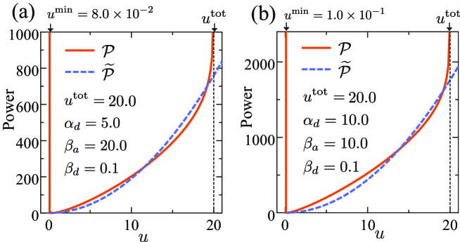
Figure 3: Exact representation of the power $\mathcal{P}$ (solid line) and its quadratic approximation $\widetilde{\mathcal{P}}$ (dashed line). (a) $u^{\mathrm{tot}}=20.0$, $\alpha_{d}=5.0$, $\beta_{a}=20.0$, and $\beta_{d}=0.1$ ($q=1.9$ for quadratic); and (b) $u^{\mathrm{tot}}=20.0$, $\alpha_{d}=10.0$, $\beta_{a}=10.0$, and $\beta_{d}=0.1$ ($q=4.4$ for quadratic). We use $k_{B}=1$ and $\mathcal{T}=1$, without loss of generality.

2.4 Finding the optimal signaling pattern

We wish to obtain the optimal control $u(t)$ that minimizes $R$ of Eq. (1) while satisfying Eq. (4) and the predefined target mean concentration of Eq. (2) [$\mu_{i_{\mathrm{out}}}(T)=z_{i_{\mathrm{out}}}(T)=\mu_{i_{\mathrm{out}}}^{\mathrm{trg}}$]. Then, by virtue of optimal control theory [23, 24], we minimize the following augmented performance index:

$$\widetilde{R} =\gamma_{i_{\mathrm{out}}}(T)+w\widetilde{\Pi}+\nu\left(z_{i_{\mathrm{out}}}(T)-\mu_{i_{\mathrm{out}}}^{\mathrm{trg}}\right)+\sum_{i=1}^{M}\int_{0}^{T}\lambda_{i}\left(h_{i}(\boldsymbol{z},u)-\dot{z}_{i}\right)dt,$$ (12)

where $\nu$ and $\boldsymbol{\lambda}=(\lambda_{1},\lambda_{2},...,\lambda_{M})$ are Lagrange multipliers that force the constraints. In Eq. (12), the exact energetic cost $\Pi$ in $R$ is replaced by its quadratic approximation $\widetilde{\Pi}$ (we set $q=1$, because the scaling of $q$ is offset by $w$). Using the calculus of variations [23, 24], finding an optimal signal $u(t)$ is reduced to solving the differential equations given by Eq. (4) and

$$\dot{\lambda}_{i}(t) =-\frac{\partial}{\partial z_{i}}H(\boldsymbol{z},u,\boldsymbol{\lambda}),$$ (13)

$$0 =\frac{\partial}{\partial u}H(\boldsymbol{z},u,\boldsymbol{\lambda}),$$ (14)

where $H(\boldsymbol{z},u,\boldsymbol{\lambda})$ is the Hamiltonian [23, 24]:

$$H(\boldsymbol{z},u,\boldsymbol{\lambda})=w\widetilde{\mathcal{P}}+\sum_{i=1}^{M}\lambda_{i}h_{i}(\boldsymbol{z},u).$$

We assume vanishing initial values for all moments: $\mu_{i}(0)=0$, $\gamma_{i}(0)=0$, and $\rho_{ij}(0)=0$ [i.e., $z_{i}(0)=0$ for all $i$]. For the boundary conditions, $\lambda_{N+i_{\mathrm{out}}}(T)=1$ and $\lambda_{i}(T)=0$ ($i\neq i_{\mathrm{out}},N+i_{\mathrm{out}}$) are required from the optimal control theory, and $z_{i_{\mathrm{out}}}(T)=\mu_{i_{\mathrm{out}}}^{\mathrm{trg}}$ for the final value of $z_{i}$. There are boundary conditions at both $t=0$ and $t=T$; this two-point boundary value problem can be solved numerically by using general solvers (see the supplementary material).

3 Results

We consider the following activation-deactivation decoding motif (Fig. 1(b)): an inactive molecule $\overline{X}_{1}$ is activated to become $X_{1}$, where the activation is dependent on the input molecule $U$. The rate equation is $\dot{x}_{1}=\alpha_{1}u\left(x_{1}^{\mathrm{tot}}-x_{1}\right)-\beta_{1}x_{1}$, where $x_{1}^{\mathrm{tot}}$ is the total concentration $x_{1}^{\mathrm{tot}}=x_{1}+\overline{x}_{1}$ which does not change with time ($\overline{x}_{1}$ is the concentration of $\overline{X}_{1}$), and $\alpha_{1}$ and $\beta_{1}$ are activation and deactivation rates, respectively. The activated molecule $X_{1}$ activates an output molecule $X_{2}$ (e.g. an activated transcription factor), and hence $X_{2}$ reports the result (i.e., $i_{\mathrm{out}}=2$). The rate equation is $\dot{x}_{2}(t)=\alpha_{2}^{0}x_{1}(x_{2}^{\mathrm{tot}}-x_{2})-\beta_{2}x_{2}$, where $x_{2}^{\mathrm{tot}}=x_{2}+\overline{x}_{2}$, and $\alpha_{2}^{0}$ and $\beta_{2}$ are activation and deactivation rates, respectively ($\overline{x}_{2}$ is the concentration of $\overline{X}_{2}$). When $x_{2}$ is far from its saturation concentration, activation of $X_{2}$ is approximately the first-order reaction with respect to $X_{1}$, i.e., $\dot{x}_{2}=\alpha_{2}x_{1}-\beta_{2}x_{2}$ where $\alpha_{2}=\alpha_{2}^{0}x_{2}^{\mathrm{tot}}$. Then dynamics of $X_{1}$ and $X_{2}$ is represented by the following linear differential equation:

$$\dot{x}_{1}(t) =\alpha_{1}u\left(x_{1}^{\mathrm{tot}}-x_{1}\right)-\beta_{1}x_{1},$$ (15)

$$\dot{x}_{2}(t) =\alpha_{2}x_{1}-\beta_{2}x_{2}.$$ (16)

Because of the linearity of Eqs. (15) and (16), the moment equation can be obtained without the truncation approximation . As denoted above, the input signal $u(t)$ must produce the dynamics that satisfy the constraint that the target mean concentration of $X_{2}$ at time $t=T$ is $\mu_{2}^{\mathrm{trg}}$ ($i_{\mathrm{out}}=2$ in Eq. (2)). This type of decoding motif is prevalent and can be found in various biochemical systems [39, 40, 41, 13]. We call this a two-stage model. By incorporating intrinsic noise due to a small number of molecules, we have a corresponding FPE from Eq. (3) (see the supplementary material). We then calculate the moment equation from the FPE.

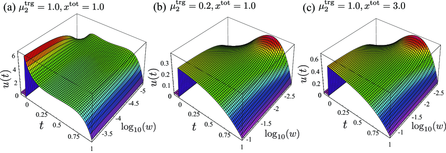
Figure 4: Optimal signal $u(t)$ for the two-stage model as a function of $t$ and $\log_{10}(w)$ for three cases: (a) $\mu_{2}^{\mathrm{trg}}=1.0$ and $x_{1}^{\mathrm{tot}}=1.0$, (b) $\mu_{2}^{\mathrm{trg}}=0.2$ and $x_{1}^{\mathrm{tot}}=1.0$, and (c) $\mu_{2}^{\mathrm{trg}}=1.0$ and $x_{1}^{\mathrm{tot}}=3.0$. The range of $w$ is $6.0\times 10^{-6}\leq w\leq 6.0\times 10^{-4}$ ($-5.22\leq\log_{10}w\leq-3.22$) for (a), $1.2\times 10^{-3}\leq w\leq 1.2\times 10^{-1}$ ($-2.92\leq\log_{10}w\leq-0.92$) for (b), and $1.7\times 10^{-3}\leq w\leq 1.7\times 10^{-1}$ ($-2.77\leq\log_{10}w\leq-0.77$) for (c). The other parameters are $\alpha_{1}=2.0$, $\alpha_{2}=2.0$, $\beta_{1}=1.0$, $\beta_{2}=1.0$, $Q=0.001$, and $T=1.0$.

3.1 Steep pattern minimizes energetic cost, and gradual pattern minimizes uncertainty

Using the two-stage model, we calculated the optimal signal $u(t)$. Figures 4(a)–(c) shows the optimal signal $u(t)$ as a function of $t$ and $\log_{10}(w)$ for three settings: (a) $\mu_{2}^{\mathrm{trg}}=1.0$ and $x_{1}^{\mathrm{tot}}=1.0$, (b) $\mu_{2}^{\mathrm{trg}}=0.2$ and $x_{1}^{\mathrm{tot}}=1.0$, and (c) $\mu_{2}^{\mathrm{trg}}=1.0$ and $x_{1}^{\mathrm{tot}}=3.0$. Note that $\mu_{2}^{\mathrm{trg}}=1.0$ is a near-saturation value with $x_{1}^{\mathrm{tot}}=1.0$, i.e., it is close to the maximal reachable target concentration. The other parameters are shown in the caption of Fig. 4. The minimum value for $w$ is determined such that $u(t)$ satisfies $u(t)\geq 0$, and the maximum is $10^{2}$ times the minimum . In all the three cases [Figs. 4(a)–(c)], for larger values of $w$, we see that the optimal signals steeply increase at $t=0$ and gradually decay as time elapses. As $w$ decreases, the optimal pattern varies from steeper to more-gradual patterns. Comparing Figs. 4(a) and (b), we can see the effect of different target concentrations. The target concentration for Fig. 4(b) is lower than it is for (a) (the other parameters are the same). For Fig. 4(a), the decay right after $t=0$ is especially rapid, and this is followed by a plateau state ($t=0.2$–$0.8$); this is a typical overshooting pattern, similar to that shown in Fig. 2(c). However, the optimal signal of Fig. 4(b) does not exhibit overshooting. We next compared Figs. 4(a) and (c) when all parameters are identical except for $x_{1}^{\mathrm{tot}}$ [$x_{1}^{\mathrm{tot}}$ for Fig. 4(c) is larger than it is for (a)] to see how the overshooting pattern depends on the total concentration $x_{1}^{\mathrm{tot}}$. When the total concentration $x_{1}^{\mathrm{tot}}$ is larger, the optimal signal does not overshoot. From these results, we see that the steep pattern minimizes the energy, whereas the gradual pattern minimizes the variance. Along with the condition of the steep pattern, the overshooting pattern emerges when the target concentration $\mu_{2}^{\mathrm{trg}}$ is relatively high and the total concentration $x_{1}^{\mathrm{tot}}$ is relatively low.

In Fig. 5(a), we compared the optimal signal (solid line), which exhibits the overshooting pattern, with a constant signal (dashed line), for the period starting at $t=0$ and ending at $t=T$; both patterns attain the same target concentration $\mu_{2}^{\mathrm{trg}}=1.0$ ($w=1.0$ for the optimal signal, which is large enough to show overshooting; the other parameters are the same as in Fig. 4(a)). Although in the interval $t=0$–$0.2$, the concentration of the optimal signal is larger than that of the constant signal, the optimal one yields a smaller concentration for $t>0.2$. The energy (quadratic approximation) of the optimal signal is $\widetilde{\Pi}_{\mathrm{opt}}=9.02$ whereas that of the constant one is $\widetilde{\Pi}_{\mathrm{const}}=10.77$ and thus the ratio is $\widetilde{\Pi}_{\mathrm{opt}}/\widetilde{\Pi}_{\mathrm{const}}=0.84$. We also calculated the ratio for the exact energy definition $\Pi$ (parameter details are the same as in Fig. 3(a)) and we obtained $\Pi_{\mathrm{opt}}/\Pi_{\mathrm{const}}=0.83$, where $\Pi_{\mathrm{opt}}$ and $\Pi_{\mathrm{const}}$ are defined analogously. Therefore the optimal signal obtained by the quadratic approximation is energetically efficient with the exact definition.

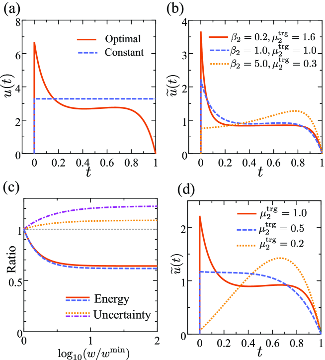
Figure 5: Results of the two-stage model. (a) Comparison of the optimal signal (solid line) and a constant signal (dashed line), which attain the same target concentration $\mu_{2}^{\mathrm{trg}}=1.0$ ($w=1.0$ for the optimal signal). (b) Normalized signal $\widetilde{u}(t)$ for three values of $\beta_{1}$: $\beta_{2}=0.2$ and $\mu_{2}^{\mathrm{trg}}=1.6$ (solid line), $\beta_{2}=1.0$ and $\mu_{2}^{\mathrm{trg}}=1.0$ (dashed line), and $\beta_{2}=5.0$ and $\mu_{2}^{\mathrm{trg}}=0.3$ (dotted line). We set $w=1.0$. (c) Energy and uncertainty dependence on $w$ for two cases: $\mu_{2}^{\mathrm{trg}}=0.2$, $\alpha_{1}=2.0$, $\alpha_{2}=2.0$, $\beta_{1}=1.0$, and $\beta_{2}=1.0$ [parameters are the same as those in Fig. 4(b); solid (energy) and dotted (uncertainty) lines] and $\mu_{2}^{\mathrm{target}}=0.5$, $\alpha_{1}=0.5$, $\alpha_{2}=10.0$, $\beta_{1}=0.1$, and $\beta_{2}=0.1$ [dashed (energy) and dot-dashed (uncertainty) lines]. Ranges of $w$ are $1.2\times 10^{-3}\leq w\leq 1.2\times 10^{-1}$ for the former and $0.03\leq w\leq 3.0$ for the latter. We plot the ratio of energy and uncertainty to those at the minimum weight $w^{\min}$. (d) Variation of the normalized signal $\widetilde{u}(t)$ in response to the target concentration $\mu_{2}^{\mathrm{trg}}$ for $w=1.2\times 10^{-3}$: $\mu_{2}^{\mathrm{trg}}=0.2$ (dotted line), $0.5$ (dashed line), and $1.0$ (solid line). In (a)–(d), the unspecified parameters are the same as those in Fig. 4(a).

3.2 Slow relaxation of the decoder causes overshooting

We considered the effects of time scale of the decoder on overthooting of the optimal signal. When increasing (decreasing) $\beta_{1}$ or $\beta_{2}$, the relaxation time of the decoder becomes shorter (longer). We first varied $\beta_{2}$ while keeping other parameters unchanged, except for $\mu_{2}^{\mathrm{trg}}$ (the other parameters are the same as those in Fig. 5(a)). Since we are interested in the shape rather than the magnitude, we normalized the signal as follows: $\widetilde{u}(t)=u(t)/\sqrt{\widetilde{\Pi}}$, which guarantees the unit energy $\widetilde{\Pi}=1$. Figure 5(b) shows the normalized signal $\widetilde{u}(t)$ for three cases: $\beta_{2}=0.2$ (solid line), $\beta_{2}=1.0$ (dashed line), and $\beta_{2}=5.0$ (dotted line). As shown above, the overshooting pattern emerges when $\mu_{2}^{\mathrm{trg}}$ is close to the saturation value. Thus, for each $\beta_{2}$ value, $\mu_{2}^{\mathrm{trg}}$ is set to near the maximal reachable value (parameter details are shown in the caption of Fig 5(b)). When $\beta_{2}=5.0$, the optimal signal does not overshoot, but the other two settings do. From this result, when the relaxation time of $X_{2}$ is sufficiently shorter than $T$, the steep (overshooting) pattern does not minimize energy consumption. The same calculation was performed for $\beta_{1}$ and we found that all of the optimal signals exhibit the overshooting (see the supplementary material). This implies that the relaxation time of $X_{1}$ is not responsible for the overshooting pattern.

3.3 Tradeoff between energy and uncertainty

In Fig. 5(c), we next evaluated the dependence on the weight $w$ of the energy $\widetilde{\Pi}$ and the uncertainty $\gamma_{i_{\mathrm{out}}}(T)$ for two parameter settings. Parameters of the first setting is the same as those in Fig. 4(b) whose results are plotted by solid (energy) and dotted (uncertainty) lines. The second setting highlights the uncertainty variation when we change $w$ and these results are shown by dashed (energy) and dot-dashed (uncertainty) lines (parameter details are described in the caption of Fig. 5(c)). In Fig. 5(c), we plot the ratio of the energy and uncertainty to those at the minimum weight $w^{\min}$, where $w^{\min}$ is the minimum of $w$ for each parameter setting. For the both settings, as $w$ increases, the uncertainty increases, and the energy decreases; there is thus a tradeoff between the energy and the uncertainty, since they cannot be minimized simultaneously. For cellular inference, the tradeoff between uncertainty and energy consumption has been confirmed by several studies [42, 43, 44, 45]. Similarly, in biochemical clocks, it has been shown that there is a tradeoff between temporal accuracy and energy consumption [46]. These studies [43, 44, 45, 46] calculated the entropy production, which is the energy required for maintaining a system at NESS. There is also a tradeoff between the energy cost and information coding in neural systems ([20] and references therein). We have shown that a similar relation also holds for dynamical signals.

3.4 Calculation with simplified model

We identified that the steep (overshooting) pattern minimizes the energy. Let us explain this mechanism with a simplified two-stage model:

$$\dot{x}_{1}(t)=u(t),\hskip 10.00002pt\dot{x}_{2}(t)=\alpha_{2}x_{1}-\beta_{2}x_{2},$$ (17)

along with a delta-function stimulus, $u(t)=\delta(t-t_{s})$ [$t_{s}$ is the time of the stimulus, where $0<t_{s}<T$]. From Eq. (17), the final output concentration is

$$x_{2}(T)=\frac{\alpha_{2}}{\beta_{2}}\left\{1-e^{-\beta_{2}\left(T-t_{s}\right)}\right\}.$$ (18)

When the relaxation of $X_{2}$ is very slow ($\beta_{2}^{-1}\gg T$), the output concentration is $x_{2}(T)\simeq\alpha_{2}(T-t_{s})$, which shows that the signal at an earlier time has a greater effect than at a later time; the steep pattern allows the output concentration to reach the target concentration at a lower cost. For the fast relaxation case ($\beta_{2}^{-1}\ll T$), we obtain $x_{2}(T)\simeq\alpha_{2}\beta_{2}^{-1}$, which shows that $x_{2}(T)$ does not depend on $t_{s}$; it is not advantageous for the signal to have a peak at an earlier time. Therefore, when the relaxation time of the decoder is very fast, the steep pattern does not confer advantages for minimizing the energy consumption; this agrees with the optimal control calculation shown in Fig. 5(b). Next, suppose there is only a single stage required to decode the signal $\dot{x}_{1}(t)=u(t)$, where $x_{1}(T)$ is the output concentration (a single-stage model). In this case, the final output concentration is $x_{1}(T)=1$ and does not depend on $t_{s}$, implying that the steep patterns do not minimize the energy. On the other hand, when there is a third stage $\dot{x}_{3}=\alpha_{3}x_{2}-\beta_{3}x_{3}$ in addition to Eqs. (17) (a three-stage model), we find that the final concentration $x_{3}(T)$ depends on $t_{s}$, unless $\beta_{2}^{-1},\beta_{3}^{-1}\ll T$ [for $\beta_{2}^{-1},\beta_{3}^{-1}\gg T$, we have $x_{3}(T)\simeq\alpha_{2}\alpha_{3}(T-t_{s})^{2}/2$, and for $\beta_{2}^{-1},\beta_{3}^{-1}\ll T$, $x_{3}(T)=\alpha_{2}\alpha_{3}/(\beta_{2}\beta_{3})$]. Thus, the steep patterns generally minimize the energy consumption when the relaxation of the decoder is slow and there are more than two stages in the decoding.

The effect of the gradual pattern can be accounted for by the moment equation. The variance $\gamma_{2}$ and covariance $\rho_{12}$ are governed by (cf. moment equations in the supplementary material)

$$\dot{\gamma}_{2}(t) =2\left(\alpha_{2}\rho_{12}-\beta_{2}\gamma_{2}\right)+2Q\left(\alpha_{2}\mu_{1}+\beta_{2}\mu_{2}\right),$$ (19)

$$\dot{\rho}_{12}(t) =\alpha_{2}\gamma_{1}-\rho_{12}\left(\alpha_{1}u+\beta_{1}+\beta_{2}\right).$$ (20)

We find that the main reason for the difference between the variance $\gamma_{2}(T)$ of the steep and gradual patterns is the area $\int_{0}^{T}\rho_{12}(t)dt$; namely, a smaller area yields a smaller value for $\gamma_{2}(T)$. From Eq. (20), because the decay velocity of $\rho_{12}(t)$ depends on $u$, a higher concentration of $u$ at a later time results in a smaller value for $\rho_{12}(t)$, which corresponds to the gradual pattern of $u(t)$.

4 Discussion and Conclusion

Our result provides insights into experimentally observed dynamical patterns. Reference [8] reported the dynamical pattern of ERK activity in response to different strengths of extracellular stimulus (i.e., the ligand concentration); the pattern is steep when stimulated by a strong stimulus, and it is gradual when stimulated by a weak one. This experimental observation can be accounted for by our model. We show that the optimal signal is steep for larger values of $\mu_{2}^{\mathrm{trg}}$ and gradual for smaller values (Fig. 5(d)). It is expected that the strong and weak ligand stimuli result in strong and weak responses, respectively, i.e., higher and lower output concentrations. Therefore, the ERK activity induced by the strong ligand stimulus may be related to $\mu_{2}^{\mathrm{trg}}=1.0$, and that induced by the weak one is related to $\mu_{2}^{\mathrm{trg}}=0.2$. When the target concentration is higher (i.e., $\mu_{2}^{\mathrm{trg}}=1.0$), the magnitude of the signal is larger, and hence the effect of the energy of the signal on the objective function $R$ (Eq. (1)) is greater than that of the variance $\gamma_{2}(T)$. In contrast, for the smaller values of $\mu_{2}^{\mathrm{trg}}$ (i.e., $\mu_{2}^{\mathrm{trg}}=0.2$), the variance $\gamma_{2}(T)$ becomes the leading term because the energy of the signal is smaller. Therefore, the steep pattern is preferable when the target concentration is higher, while the gradual one is preferable when the target concentration is lower. These theoretical results qualitatively agree with the observed dynamical patterns reported in Ref. [8].

Along with conditions for the steep pattern, the overshooting dynamics minimize the energy of the input signals when the total concentration $x_{1}^{\mathrm{tot}}$ is smaller and the target concentration $\mu_{i_{\mathrm{out}}}^{\mathrm{trg}}$ is higher. Surprisingly, this behavior can be found in several dynamical patterns; for example, activities of the ERK, the I$\kappa$B kinase (IKK), which regulates the transcription factor NF-$\kappa$B, and the kinase AKT show this behavior [47, 39, 48, 4, 49]. These examples indicate that the pattern has biological advantages. We also note the biochemical origin of the overshoot. For example, simple incoherent feed-forward loops [50, 51, 1, 2] and activation-deactivation motifs [52] can generate such a pattern, and these motifs can indeed be found in signaling pathways. Furthermore, a strongly damped oscillation is indistinguishable from overshooting. Although NF-$\kappa$B is known to exhibit damped oscillation upon stimulation, some studies [53, 54] are skeptical about the functional role of the NF-$\kappa$B oscillation; that is, the NF-$\kappa$B oscillation may be a by-product of inducing overshooting. Overshooting has often been observed in actual dynamical patterns, but its functional advantage has not been well understood. We have shown that this pattern produces direct benefits.

References

- [1] Alon U 2007 Nat. Rev. Genet. 8 450–461
- [2] Alon U 2007 An Introduction to Systems Biology (CRC Press)
- [3] Behar M and Hoffmann A 2010 Curr. Opin. Genetics Dev. 20 684–693
- [4] Kubota H, Noguchi R, Toyoshima Y, Ozaki Y i, Uda S, Watanabe K, Ogawa W and Kuroda S 2012 Mol. Cell 46 820–832
- [5] Purvis J E, Karhohs K W, Mock C, Batchelor E, Loewer A and Lahav G 2012 Science 336 1440–1444
- [6] Purvis J E and Lahav G 2013 Cell 152 945–956
- [7] Sonnen K F and Aulehla A 2014 Sem. Cell. Dev. Biol. 34 91–98
- [8] Selimkhanov J, Taylor B, Yao J, Pilko A, Albeck J, Hoffmann A, Tsimring L and Wollman R 2014 Science 346 1370–1373
- [9] Lin Y, Sohn C H, Dalal C K, Cai L and Elowitz M B 2015 Nature 527 54–58
- [10] Tostevin F and ten Wolde P R 2009 Phys. Rev. Lett. 102 218101
- [11] Mora T and Wingreen N S 2010 Phys. Rev. Lett. 104 248101
- [12] Mugler A, Walczak A M and Wiggins C H 2010 Phys. Rev. Lett. 105 058101
- [13] Hansen A S and O’Shea E K 2013 Mol. Syst. Biol. 9 704
- [14] Kobayashi T J 2010 Phys. Rev. Lett. 104 228104
- [15] Mc Mahon S S, Lenive O, Filippi S and Stumpf M P H 2015 J. R. Soc. Interface 12 20150597
- [16] Becker N B, Mugler A and ten Wolde P R 2015 Phys. Rev. Lett. 115 258103
- [17] Makadia H K, Schwaber J S and Vadigepalli R 2015 PLoS Comput. Biol. 11 e1004563
- [18] Tostevin F, de Ronde W and ten Wolde P R 2012 Phys. Rev. Lett. 108 108104
- [19] Laughlin S B 2001 Curr. Opin. Neurobiol. 11 475–480
- [20] Sengupta B and Stemmler M B 2014 Proc. IEEE 102 738–750
- [21] Mehta P, Lang A H and Schwab D J 2016 J. Stat. Phys. 162 1153–1166
- [22] McDonnell M D, Stocks N G, Pearce C E M and Abbott D 2008 Stochastic resonance (Cambridge University Press)
- [23] Kamien M I and Schwartz N L 2012 Dynamic optimization: the calculus of variations and optimal control in economics and management (Dover Publications)
- [24] Hull D G 2013 Optimal control theory for applications (Springer Science & Business Media)
- [25] Gillespie D T 2000 J. Chem. Phys. 113 297–306
- [26] Klipp E, Liebermeister W, Wierling C, Kowald A, Lehrach H and Herwig R 2013 Systems Biology (Wiley-Blackwell)
- [27] Forger D B and Paydarfar D 2004 J. Theol. Biol. 230 521–532
- [28] Moehlis J, Shea-Brown E and Rabitz H 2006 J. Comput. Nonlin. Dyn. 1 358–367
- [29] Hasegawa Y and Arita M 2014 J. R. Soc. Interface 11 20131018
- [30] Hasegawa Y and Arita M 2014 Phys. Rev. Lett. 113 108101
- [31] Iolov A, Ditlevsen S and Longtin A 2014 J. Neural Eng. 11 046004
- [32] Rodriguez R and Tuckwell H C 1996 Phys. Rev. E 54 5585–5590
- [33] Tuckwell H C and Jost J 2009 Physica A 388 4115–4125
- [34] Qian H and Beard D A 2005 Biophys. Chem. 114 213–220
- [35] Qian H 2007 Annu. Rev. Phys. Chem. 58 113–142
- [36] Beard D A and Qian H 2008 Chemical biophysics: quantitative analysis of cellular systems (Cambridge University Press)
- [37] Aksan Kurnaz I 2004 Biotechnol. Bioeng. 88 890–900
- [38] Thomson T M, Benjamin K R, Bush A, Love T, Pincus D, Resnekov O, Yu R C, Gordon A, Colman-Lerner A, Endy D and Brent R 2011 Proc. Natl. Acad. Sci. U.S.A. 108 20265–20270
- [39] Sasagawa S, Ozaki Y i, Fujita K and Kuroda S 2005 Nat. Cell. Biol. 7 365–373
- [40] Salazar C, Politi A Z and Höfer T 2008 Biophys. J. 94 1203–1215
- [41] Tănase-Nicola S, Warren P B and ten Wolde P R 2006 Phys. Rev. Lett. 97 068102
- [42] Tu Y 2008 Proc. Natl. Acad. Sci. U.S.A. 105 11737–11741
- [43] Mehta P and Schwab D J 2012 Proc. Natl. Acad. Sci. U.S.A. 109 17978–17982
- [44] Lang A H, Fisher C K, Mora T and Mehta P 2014 Phys. Rev. Lett. 113 148103
- [45] Barato A C, Hartich D and Seifert U 2014 New J. Phys. 16 103024
- [46] Cao Y, Wang H, Ouyang Q and Tu Y 2015 Nat. Phys. 11 772–778
- [47] Werner S L, Barken D and Hoffmann A 2005 Science 309 1857–1861
- [48] Werner S L, Kearns J D, Zadorozhnaya V, Lynch C, O’Dea E, Boldin M P, Ma A, Baltimore D and Hoffmann A 2008 Genes & Development 22 2093–2101
- [49] Mathew S, Sundararaj S, Mamiya H and Banerjee I 2014 Bioinformatics 30 2334–2342
- [50] Mangan S and Alon U 2003 Proc. Natl. Acad. Sci. U.S.A. 100 11980–11985
- [51] Mangan S, Itzkovitz S, Zaslaver A and Alon U 2006 J. Mol. Biol. 356 1073–1081
- [52] Behar M and Hoffmann A 2013 Biophys. J. 105 231–241
- [53] Barken D, Wang C J, Kearns J, Cheong R, Hoffmann A and Levchenko A 2005 Science 308 52–52
- [54] Cheong R, Hoffmann A and Levchenko A 2008 Mol. Syst. Biol. 4 192