Transport properties of a charged hot spot in an external electromagnetic field

Abstract

We investigate adiabatic expansion of a charged and rotating fluid element consisting of weakly interacting particles, which is initially perturbed by an external electromagnetic field. A framework for the perturbative calculation of the non-equilibrium distribution function of this fluid volume is considered and the distribution function is calculated to the first order in the perturbative expansion. This distribution function, which describes the evolution of the element with constant entropy, allows to calculate momentum flux tensor and viscosity coefficients of the expanding system. We show, that these viscosity coefficients depend on the initial angular velocity of the spot and on the strength of its initial perturbation by the external field. Obtained results are applied to the phenomenology of the viscosity to the entropy ratio calculated in lattice models.

1 Introduction

Collisions of relativistic nuclei in the RHIC and LHC experiments at very high energies led to the discovery of a new state of matter named quark-gluon plasma (QGP). At the initial stages of the scattering, this plasma resembles almost an ideal liquid which microscopic structure is not yet well understood [1, 2, 3, 4, 5, 6, 7, 8, 9]. The data obtained at the RHIC experiments is in a good agreement with the predictions of the ideal relativistic fluid dynamics, [10, 11, 12], that establish fluid dynamics as the main theoretical tool to describe collective flow in the collisions. As an input to the hydrodynamical evolution of the particles it is assumed that after a very short time, $\tau\,<\,1\,\,fm/c$ [12], the matter reaches a thermal equilibrium and expands with a very small shear viscosity [13, 14].

Different models of QGP were proposed in order to describe its fluid behavior. Among other there are strongly coupled Quark Gluon Plasma (sQGP) model, see [1] and references therein, different non-perturbative and lattice models [15, 16, 17, 18]. In our approach we will model a QGP system created in the process of high-energy scattering as a system of weakly interacting particles where the thermal equilibrium is achieved for a small elements of the colliding matter [3, 8, 14, 19, 20] separately at some initial moments of time. Namely, we assume, that the whole colliding system is not in a global equilibrium state, see [3, 21], and therefore, at the initial stages of the evolution, only local equilibrium may be achieved for the small fluid elements of the matter, independently on each other in the first approximation, see [22]. We can call these elements as hot spots, considering them as local initial fluctuations of the density, see for example [23, 24, 25, 26, 27], and which can be related with the physics of saturation, [28, 29, 30, 31, 32], as well. Consequently, accordingly to [33], the expansion of the dense initial fluctuation occurs with the constant entropy which justifies the applicability of the hydrodynamical description of the process. This adiabatic expansion continues till the value of the particle’s mean free path inside the expanding hot spot becomes comparable to the size of the whole system. At this stage, instead of liquid, there appears a gas of interacting particles with rapidly decreasing density, see for example [34].

In kinetic approach the process of the dense system expansion, i.e. hydrodynamics flow, is described by the Vlasov’s equation. This equation determines a microscopic distribution function for the fluid element which depends on time in the case of non-equilibrium processes. For the very dense system the applicability of Vlasov’s equation is determined by the value of plasma parameter, the dynamical constraints on the value of this parameter coincide with the requests of the mean free path smallness introduced in [33]. Additionally, an application of the fluid dynamics to the process of the hot spot expansion requires some initial conditions among which the most intriguing one is a condition of a small value of the shear viscosity/entropy ratio. For the collective flow, described by Vlasov’s equation, usual perturbative mechanisms, see [35], responsible for the shear viscosity value are absent. Indeed, in the Vlasov’s equation framework, in the first approximation in the plasma parameter, the collision term is zero implying an entropy conservation and collective flow of the particles without rescattering. To resolve this problems of the collective flow of an almost ideal fluid with very small viscosity coefficients some new mechanisms of the shear viscosity smallness were proposed, see [36, 37, 38, 39, 40]. Additionally, for the non-isotropic initial conditions, the connection between stress-energy tensor and viscosity is more complicated than in the case of isotropic initial state, see [34] for example, that means an existence of a family of different viscosity coefficients in the expanding system, for example see [36] or [49].

Referring to Vlasov’s equation as to the equation which describes equilibrium state only, the viscosity coefficients will be equal zero by definition. Therefore some time-dependent fluctuations around the equilibrium must be considered in the approach in order to generate the viscosity coefficients. The mechanisms behind these fluctuations may be, for example, some instabilities generated in the plasma, see [37, 38, 39, 40] and references therein. The viscosity obtained by this way is called ”anomalous” one, in contrast to viscosity coefficient created by the perturbative rescattering mechanisms as in [35]. The proposed generation of ”anomalous” viscosity and corresponding solution of Vlasov’s equation, in turn, requires an existence of some equilibrium state which is perturbed by fluctuations, but in the case of very fast expanding hot spot such set-up may be questionable.

In this paper we continue to develop a model proposed in [22, 42]. Namely, we assume that the local energy density fluctuations, charged hot spots, see [23, 24, 25, 26, 27] and also [41, 19], are created at the very initial stage of interactions at time $\tau\,<\,0.5\,fm/c\,$, see [12, 14, 15, 19, 22, 43]. These fluctuations are very dense and small, whose size is much smaller than the proton size, see [19, 22], with energy density is much larger than the density achieved in high-energy interactions at the energies $\sqrt{s}\,<\,100\,GeV\,$. In our model we assume that the hot spots consist of the particles with weak inter-particle interactions and have a non-zero charge. The small coupling constant approximation makes our model useful for the electromagnetic type of interactions or for the modeling of the interactions of asymptotically free quarks and gluons in QCD. In the later case, this expanding fluid element can be considered as local colored density fluctuation, see [43, 44] for example. Therefore, we consider our model as some ”toy” model for the real QCD processes, which applicability is justified by the smallness of the strong coupling constant in the case of a fluctuation with $0.05\,-\,0.5\,fm$ size, see [22]. In our model we assume also, that the charged hot spot is perturbated by the external field at the initial moment of time, and only then the fluctuation is expanding with relativistic velocity along z axis. Thus, consequently, further hot spot’s evolution is considered as an adiabatic expansion of the very dense drop of matter, which kinetic description is given by a non-stationary solution of Vlasov’s equation with some inhomogeneous initial conditions. In this model, for the simplicity, we consider only one kind of charge, nevertheless the generalization to the case of many charges is straightforward. As the initial condition for the expansion, we choose a ”rigid body” condition, see [53, 42], where the whole fluid element is rotating with some angular velocity. The value of the angular velocity is a parameter of the model which we can vary, it’s emergence may be understood as consequence of the interaction of the charged fluctuation with crossed electrical and magnetic fields at the initial moment of time, see [53]. Thus, in addition to the parameter which characterizes interaction of the hot spot with the external field, another degree of freedom is introduced in the model. As we will see further, those two new degrees of freedom determine leading values of the viscosity coefficients.

In the next Section 2, we discuss the form of Vlasov’s equation, its integral representation and perturbative framework for the solution as well as a form of the external electromagnetic field. In Section 3 we solve Vlasov’s equation and calculate mean velocities of the expanding hot spot in the leading order of the perturbation. Section 4 is dedicated to the calculation of the momentum flux tensor and viscosity coefficients of the system, whereas in the Section 5 the values of the shear viscosity coefficients at different values of the problem’s parameters as functions of time are present. In the Section 6 we determine the form the viscosity coefficients dependence on temperature and present the calculation of the ratios of the viscosity coefficients to the entropy as functions of temperature in comparison with the lattice data. The Conclusions are presented in Section 7.

2 Vlasov’s equation for a charged hot spot in electromagnetic field

2.1 Vlasov’s equations system

In this section we review main results of [42] for Vlasov’s equation. The usual form of Vlasov’s equation for a system of charged particles in an external electromagnetic field is given by

$$\frac{\partial\,f_{s}}{\partial\,t}\,+\,\vec{v}\,\frac{\partial\,f_{s}}{\partial\vec{r}}\,+\,\left(\,q\vec{E}\,+\,\frac{q}{c}\,\vec{v}\times\vec{B}\right)\,\frac{\partial\,f_{s}}{\partial\vec{p}}\,=\,0\,.$$ (1)

In a case of non-stationary processes the equation must be solved together with Maxwell’s equations

$$\nabla\times\vec{E}\,=\,-\frac{1}{c}\,\frac{\partial\vec{B}}{\partial t}\,,$$ (2)

$$\nabla\times\vec{B}\,=\,\frac{1}{c}\,\frac{\partial\vec{E}}{\partial t}\,+\,\frac{4\pi\,}{c}\,\vec{j}\,=\,\frac{1}{c}\,\frac{\partial\vec{E}}{\partial t}\,+\,\frac{4\pi\,q\,n\,}{c}\,\langle\,\vec{v}\,\rangle\,,$$ (3)

$$\nabla\cdot\,\vec{E}\,=\,4\,\pi\,q\,n\,\int\,f_{s}(\vec{r},\,\vec{p},\,t)\,d^{3}p\,,$$ (4)

$$\nabla\cdot\,\vec{B}\,=\,0\,,$$ (5)

where we normalize our distribution function as follows

$$\int\,f_{s}(\vec{r}=0,\,\vec{p},\,t=0)\,d^{3}p\,=\,1\,.$$ (6)

Electric and magnetic fields in Maxwell equations Eq. (2)-Eq. (5) are a combination of the self-generated electric $\vec{E}^{s}$ and magnetic $\vec{B}^{s}$ fields of the matter element and external electromagnetic field:

$$\vec{E}_{Total}\,=\,\vec{E}^{s}\,-\,\vec{E}^{ext}\,;\,\,\vec{B}_{Total}\,=\,\vec{B}^{s}\,+\,\vec{B}^{ext}\,.$$ (7)

In the next subsection we discuss the configuration of these fields.

2.2 Fields configuration

As an external electromagnetic field in the problem we consider the electromagnetic field in the transverse plan which perturbates the density fluctuation at the initial moment of time only. In the rest frame of the hot spot of interest, this field is given by the following potentials

$$\varphi(\vec{r},t)\,=\,A_{z}(\vec{r},t)\,=\,0\,,$$ (8)

$$A_{x}(\vec{r},t)\,=\,-\,2\,q\,n_{0}\,V_{0}\,\theta(z\,-\,ct)\,\partial_{x}\,K_{0}(|r_{\bot}\,-\,b|/r_{0D})\,,$$ (9)

$$A_{y}(\vec{r},t)\,=\,-\,2\,q\,n_{0}\,V_{0}\,\theta(z\,-\,ct)\,\partial_{y}\,K_{0}(|r_{\bot}\,-\,b|/r_{0D})\,,$$ (10)

see [42]. Here $r_{0D}$ is a Debye length of the incident cloud of the particles which surrounds the hot spot, see [45]-[46], $K_{0}$ is the Macdonald function and $b$ is the transverse distance between incident drop and hot spot at rest (impact parameter), in the following we consider the case $b\,=\,0$. The radial component of the 4-potential in the cylindrical coordinate system, has the following form:

$$A_{r}(\vec{r},t)\,=\,\,A_{x}(\vec{r},t)\cos\,\theta+A_{y}(\vec{r},t)\,\sin\,\theta\,,$$ (11)

thus we obtain

$$A_{r}(\vec{r},t)\,=\,-\,2\,q\,n_{0}\,V_{0}\,\theta(z\,-\,ct)\,\frac{\partial K_{0}(|r|/r_{0D})}{\partial r}\,=\,Q_{T}\,\theta(z\,-\,ct)\,K_{1}(\xi_{0})\,.$$ (12)

Here $\xi_{0}\,=\,\frac{r}{r_{0D}}$ and we defined an overall charge of the incident drop as

$$Q_{T}\,=\,q\,n_{0}\,V_{0}\,.$$ (13)

Therefore, the hot spot at rest is affected by the following external fields:

$$\vec{E}^{ext}_{r}\,=\,-\,\frac{1}{c}\frac{\partial\,A_{r}}{\partial\,t}\,\hat{e}_{r}\,=\,\frac{Q_{T}}{r_{0D}}\,\delta(ct)\,K_{1}(\xi_{0})\,$$ (14)

and

$$\vec{B}^{ext}_{\theta}\,=\frac{\partial\,A_{r}}{\partial\,z}\,\hat{e}_{\theta}\,=\,\frac{Q_{T}}{r_{0D}}\,\delta(ct)\,K_{1}(\xi_{0})\,.$$ (15)

Here we took into account, that our fluid element is at $z\,=\,0$ at the time $t\,=\,0$. We also assume axially symmetry of the problem, otherwise some dependence of $Q_{T}$ on polar angle must be introduced.

The following configuration of the self-generated fields suit our problem:

$$\vec{E}^{s}_{r}\,=\,-\,\frac{1}{c}\frac{\partial\,A_{r}^{s}}{\partial\,t}\,\hat{e}_{r}\,,\vec{E}^{s}_{\theta}\,=\,-\,\frac{1}{c}\frac{\partial\,A_{\theta}^{s}}{\partial\,t}\,\hat{e}_{\theta}\,;\,\,\,\,\,\,\,\,\,\,\,\,\,\,\,\,\,\,\,\,\,\,\,$$ (16)

$$\vec{B}^{s}_{r}\,=\,-\,\frac{\partial\,A_{\theta}^{s}}{\partial\,z}\,\hat{e}_{r}\,,\,\,\vec{B}^{s}_{\theta}\,=\,\frac{\partial\,A_{r}^{s}}{\partial\,z}\,\hat{e}_{\theta}\,,\,\,\vec{B}^{s}_{z}\,=\,\frac{1}{r}\frac{\partial\,r\,A_{\theta}^{s}}{\partial\,r}\,\hat{e}_{z}\,,$$ (17)

see [42, 53]. In general, when we consider a non-stationary problem, a formulation of Maxwell equations in terms of potentials $A_{r}\,,A_{\theta}$ is more useful. So, the following equations hold for the potentials:

$$\frac{1}{c^{2}}\frac{\partial^{2}A_{r}}{\partial t^{2}}\,-\,\frac{\partial^{2}A_{r}}{\partial z^{2}}\,=\,\frac{4\pi\,}{c}\,j_{r}\,;$$ (18)

$$\frac{1}{c^{2}}\frac{\partial^{2}A_{\theta}}{\partial t^{2}}\,-\,\frac{\partial^{2}A_{\theta}}{\partial z^{2}}\,-\,\frac{1}{r}\frac{\partial}{\partial r}\left(\,r\frac{\partial A_{\theta}}{\partial r}\right)\,+\,\frac{A_{\theta}}{r^{2}}\,=\,\frac{4\pi\,}{c}\,j_{\theta}\,;$$ (19)

$$-\frac{1}{r\,c}\frac{\partial^{2}\left(r\,A_{r}\right)}{\partial t\,\partial r}\,=\,4\pi\,q\,n\,;$$ (20)

$$\frac{1}{r}\frac{\partial^{2}\left(r\,A_{r}\right)}{\partial r\,\partial z}\,=\,\frac{4\pi\,}{c}\,j_{z}\,.$$ (21)

We obtained, that equation Eq. (18) is a one-dimensional wave equations for the potential $A_{r}\,$ with a source which may depend on the potentials of the problem. In turn, equation Eq. (19) is a kind of non-homogeneous Bessel equation for the potential $A_{\theta}\,$, where the source may depend on the potentials as well. Equations Eq. (20)-Eq. (21) have different meaning. Namely, we can rewrite them in the following form:

$$q\,\frac{\partial n}{\partial z}\,+\,\frac{1}{c^{2}}\,\frac{\partial j_{z}}{\partial t}\,=\,0\,.$$ (22)

The problem is formulated for the relativistic motion of the drop along $z$ axis when

$$j_{z}\,=\,q\,n\,<v_{z}>\,\approx\,\,q\,n\,c\,$$ (23)

implying for Eq. (22):

$$\frac{\partial n}{\partial z}\,+\,\frac{1}{c}\,\frac{\partial n}{\partial t}\,=\,0\,,$$ (24)

which is homogeneous wave equation for the wave propagation in positive $z$ direction. We see, that both Eq. (20)-Eq. (21) are simply provide a condition that to a first approximation our fluid element expands along $z$ axis with $<v_{z}>\,\approx\,c\,$ velocity .

2.3 Vlasov’s equation in integral form

In order to simplify the solution of our equation, the first step we make is a reformulation of Vlasov’s equation in terms of dimensionless variables. We introduce:

$$t\,\rightarrow\,\frac{t}{t_{0}}\,\,,\vec{r}\,\rightarrow\,\frac{\vec{r}}{l_{0}}\,\,,l_{0}\,=\,t_{0}\,c\,\,,\vec{p}\,\rightarrow\,\frac{\vec{p}}{mc}\,\,,\vec{v}\,\rightarrow\,\frac{\vec{v}}{c}\,\,,$$ (25)

where $t_{0}$ is a time of applicability of Vlasov’s equation and $l_{0}$ corresponds to this time length. So, in the following, we will understand as variables the dimensionless quantities from Eq. (25). We rewrite Eq. (1), obtaining the following equation:

$$\frac{\partial\,f_{s}}{\partial\,t}\,+\,\vec{v}\,\frac{\partial\,f_{s}}{\partial\vec{r}}\,+\,\frac{t_{0}}{mc}\,\vec{F}\,\frac{\partial\,f_{s}}{\partial\vec{p}}\,=\,0\,.$$ (26)

Further, we assume the parameter

$$\frac{t_{0}|\vec{F}|}{mc}\,\simeq\,\frac{l_{0}|\vec{F}|}{mc^{2}}\,,$$ (27)

as a perturbative parameter of the problem. In both cases, either this parameter is large or small, it can serve as the parameter for a perturbative expansion of functions. In our further calculations we take this parameter as a small one, that implies a smallness of the work of dissipative forces during the hot spot expansion relatively to its kinetic energy .

Following to [22] we rewrite the differential equation Eq. (26) in the integral form. First of all we rewrite Vlasov’s equation as

$$\,\frac{\partial\,f_{s}}{\partial\,t}\,+\,\vec{v}\,\frac{\partial\,f_{s}}{\partial\vec{r}}\,=\,-\,\frac{t_{0}\vec{F}}{mc}\,\frac{\partial\,f_{s}}{\partial\vec{p}}\,.$$ (28)

The l.h.s. of this equation we can write as the well-known transport equation, see [52], whose fundamental solution $\mathscr{E}$ satisfies

$$\,\frac{\partial\,\mathscr{E}}{\partial\,t}\,+\,\vec{v}\,\frac{\partial\,\mathscr{E}}{\partial\vec{r}}\,=\,\delta(t)\,\delta^{2}(\vec{r})\,,$$ (29)

here $\vec{r}$ is the 2-dimensional $\vec{r}\,=\,(r,z)$ vector. The fundamental solution of Eq. (29) is well known:

$$\mathscr{E}\,=\,\theta(t)\,\delta(\,r\,-\,v_{r}\,t\,)\,\delta(\,z\,-\,v_{z}\,t\,).$$ (30)

With the help of Eq. (29), we rewrite Eq. (28) as an integral equation:

$$f_{s}(\vec{r},\vec{v},t)=-\frac{t_{0}}{mc}\,\int dr^{{}^{\prime}}dz^{{}^{\prime}}dt^{{}^{\prime}}\mathscr{E}(t-t^{{}^{\prime}},\vec{r}-\vec{r}^{{}^{\prime}})\,\vec{F}(t^{{}^{\prime}},\vec{r}^{{}^{\prime}})\,\frac{\partial\,f_{s}(\vec{r}^{{}^{\prime}},\vec{v},t^{{}^{\prime}})}{\partial\vec{p}}+f_{0}(\vec{r}-\vec{v}\,t\,,\vec{v})\,,$$ (31)

where the function $f_{0}(r,\vec{\zeta})$ will be determined later. Inserting Eq. (30) into Eq. (31), we obtain:

$$f_{s}(\vec{r},\vec{v},t)\,=\,-\,\frac{t_{0}}{mc}\int_{0}^{t}dt^{{}^{\prime}}\vec{F}(t^{{}^{\prime}},\vec{r}-\vec{v}(t-t^{{}^{\prime}}))\frac{\partial\,f_{s}(\vec{r}-\vec{v}(t-t^{{}^{\prime}}),\vec{v},t^{{}^{\prime}})}{\partial\vec{p}}+\,f_{0}(\vec{r}-\vec{v}t,\vec{v}).$$ (32)

Now, our Lorentz force $\vec{F}$ consists of two parts, external one and part which corresponds to self-generated fields:

$$\vec{F}\,=\,\vec{F}^{ext}\,+\,\vec{F}^{s}\,,$$ (33)

where we have for the external part of the force in the terms of dimensionless variables:

$$F_{r}^{ext}\,=\,q\,\left(-\,E_{r}^{ext}\,-\,v_{z}\,B_{\theta}^{ext}\right)\,=\,-\,\frac{q\,Q_{T}}{l_{0}^{2}\hat{r}_{0D}}\,K_{1}(\xi_{0})\,\left(\,1\,+\,v_{z}\right)\,\delta(t)\,$$ (34)

$$F_{\theta}^{ext}\,=\,0\,,$$ (35)

$$F_{z}^{ext}\,=\,q\,\,v_{r}\,B_{\theta}^{ext}\,=\,\frac{q\,Q_{T}\,}{l_{0}^{2}\hat{r}_{0D}}\,v_{r}\,K_{1}(\xi_{0})\,\delta(t)\,,$$ (36)

with redefined $\xi_{0}$

$$\xi_{0}\,=\,\frac{|r\,-\,\hat{r}_{0D}|}{\hat{r}_{0D}}$$ (37)

and with $\hat{r}_{0D}\,=\,r_{0D}/l_{0}$. Thus using Eq. (34)-Eq. (36), we obtain for Eq. (32):

$$f_{s}(\vec{r},\vec{v},t)\,=\,-\,\frac{t_{0}}{mc}\int_{0}^{t}dt^{{}^{\prime}}\vec{F}^{s}(t^{{}^{\prime}},\vec{r}-\vec{v}(t-t^{{}^{\prime}}))\frac{\partial\,f_{s}(\vec{r}-\vec{v}(t-t^{{}^{\prime}}),\vec{v},t^{{}^{\prime}})}{\partial\vec{p}}+\,$$ (38)

$$+\frac{t_{0}}{mc}\frac{qQ_{T}}{l_{0}^{2}\hat{r}_{0D}}K_{1}(\xi_{0}(v_{r}t))\left(\frac{\partial f_{s0}(\vec{r}-\vec{v}t,\vec{v})}{\partial p_{r}}\left(1+v_{z}\right)-v_{r}\frac{\partial\,f_{s0}(\vec{r}-\vec{v}t,\vec{v})}{\partial p_{z}}\right)+f_{0}(\vec{r}-\vec{v}t,\vec{v})\,,$$

here we denoted $f_{s0}\,=\,f_{s}(\vec{r},\vec{v},t=0)$. Initial condition of the problem is provided by Eq. (38) by taking $t\,=\,0$. We have

$$f_{s0}(\vec{r},\vec{v})\,=\,\Lambda_{0}\,\left(\frac{\partial f_{s0}(\vec{r},\vec{v})}{\partial p_{r}}\left(1+v_{z}\right)-v_{r}\frac{\partial\,f_{s0}(\vec{r},\vec{v})}{\partial p_{z}}\right)+f_{0}(\vec{r},\vec{v})\,,$$ (39)

with additional small parameter of the problem

$$\Lambda_{0}\,=\,\frac{t_{0}}{mc}\frac{qQ_{T}}{l_{0}^{2}\hat{r}_{0D}}K_{1}(\xi_{0})\,=\,\frac{qQ_{T}}{mc^{2}r_{0D}}K_{1}(\xi_{0})\,<<\,1\,,$$ (40)

that value characterizes a smallness of the interaction of the charged fluctuation with the external field at the initial moment of time relative to the hot spot’s kinetic energy. Here the function $f_{0}(\vec{r},\vec{v})$ provides an initial condition for the problem in absence of external fields. An analytical solution of Eq. (39) for the $f_{s0}$ function is unknown, further we will consider only perturbative solutions of this equation.

2.4 Initial conditions for Vlasov’s equation

There are two functions which we need as initial conditions in order to solve Eq. (38), they are $f_{s0}$ and $f_{0}$. We can solve perturbatively Eq. (39) considering $\Lambda_{0}$ as a small parameter:

$$f_{s0}(\vec{r},\vec{v})\,=\,\sum_{n\,=\,0}^{\infty}\,{\Lambda_{0}^{n}}\,f_{s0n}$$ (41)

At the first order on this parameter the solution of Eq. (38) is:

$$f_{s0}(\vec{r},\vec{v})\,=\,\Lambda_{0}\,\left(\frac{\partial f_{0}(\vec{r},\vec{v})}{\partial p_{r}}\left(1+v_{z}\right)-v_{r}\frac{\partial\,f_{0}(\vec{r},\vec{v})}{\partial p_{z}}\right)+f_{0}(\vec{r},\vec{v})\,,$$ (42)

see [42]. Therefore, an important step of the problem is the choice of the initial condition for the Vlasov’s equation without an external field. So, first of all, we define the following numericall parameters:

$$\beta\,=\,|v_{z}|\,\propto\,1,\,\,\gamma\,=\,\sqrt{1-v^{2}}\,\approx\,\sqrt{1-\beta^{2}}\,<<\,1.$$ (43)

The energy of a relativistic particle is given by the following Hamiltonian:

$$H\,=\,mc^{2}\,\sqrt{1\,+\,p^{2}_{\bot}\,+\,p_{z}^{2}}\,\approx\,mc^{2}\,\sqrt{1\,+\,p_{z}^{2}}\,\left(1\,+\,\frac{p^{2}_{\bot}}{2\,\left(1\,+\,p_{z}^{2}\right)}\,\right).$$ (44)

In our notations we have:

$$p_{z}\,=\,\frac{\beta}{\gamma}\,=\,\frac{v_{z}}{\gamma}\,,\,\,\,\,p_{r}\,=\,v_{r}\,,\,\,\,\,p_{\theta}\,=\,v_{\theta}\,.$$ (45)

Thus we obtain:

$$H\,\approx\,mc^{2}\frac{\beta}{\gamma}\,+\,mc^{2}\,\frac{\gamma}{\beta}\frac{p^{2}_{\bot}}{2}\,=\,H_{\|}\,+\,H_{\bot}\,.$$ (46)

Now, following by [53], we define our initial distribution function as a kind of ”rigid-rotor” equilibrium distribution function with factorization of longitudinal and transverse velocities:

$$f_{0}(\vec{r},\vec{v})\,=\,\frac{\gamma}{\beta}\left(\frac{m^{2}c^{3}}{2\pi}\right)\,\delta\left(H_{\bot}\,-\,P_{\theta}\omega_{r}\,-\,kT_{\bot}\right)\,\delta\left(mcp_{z}\,-\,\frac{mc\beta}{\gamma}\right)\,\phi(z)\,,$$ (47)

where we adopt

$$P_{\theta}\,=\,\frac{\gamma}{\beta}\,r\,l_{0}\,mc\left(p_{\theta}\,-\,\omega_{c}\,r\,l_{0}\,/\,2c\,\right)\,,$$ (48)

with

$$\omega_{c}\,=\,\frac{|q|\,B_{z0}}{m\,c}\,.$$ (49)

Here

$$A^{0}_{\theta}\,=\,\,B_{z0}\,r\,/\,2$$ (50)

is the solution of homogeneous Eq. (19) and function $\phi(z)\,$ determines the position of the drop in the laboratory coordinate frame on the $z$ axis. We note also, that the form of Eq. (47) function is consistent with requests on microcanonical ensemble distribution function which describes an adiabatic states of the matter.

The normalization of Eq. (47) function is usual:

$$\int d^{3}p\,f_{0}(\vec{r},\vec{v})\,=\,\frac{\gamma}{\beta}\left(\frac{m^{2}c^{3}}{2\pi}\right)\,\int d^{2}p_{\bot}\,dp_{z}\,\delta\left(H_{\bot}\,-\,P_{\theta}\omega_{r}\,-\,kT_{\bot}\right)\,\delta\left(mcp_{z}\,-\,\frac{mc\beta}{\gamma}\right)\,\phi(z)\,=\,\phi(z)\,,$$ (51)

with the request $\phi(z)_{z\,=\,0}\,=\,1$. We notice also, that the integral of the delta-function in Eq. (51) is not zero only for some values of $r$. Indeed, rewriting

$$H_{\bot}-\omega_{r}\,P_{\theta}\,=\,mc^{2}\,\frac{\gamma}{2\,\beta}\left(\,p_{r}^{2}\,+\,(p_{\theta}\,-\,\frac{rl_{0}}{c}\omega_{r})^{2}\,\right)\,+\,\psi(r)\,,$$ (52)

with an effective potential $\psi(r)$

$$\psi(r)\,=\,\frac{m\,\gamma}{2\,\beta}\,\omega_{r}\,\left(\omega_{c}\,-\,\omega_{r}\right)\,r^{2}\,l_{0}^{2}\,,$$ (53)

we obtain that for the distribution function Eq. (42) the density profile is non-zero if only

$$n(r)=\left\{\begin{array}[]{rl}&1\,=\,const.,\,\,0\,\leq\,r\,<\,r_{b}\\ &0\,,\,\,\,\,\,\,\,\,\,\,\,\,\,\,\,\,\,\,\,\,\,\,\,\,\,\,\,\,\,r\,\,>\,r_{b}\,,\\ \end{array}\right.$$ (54)

where

$$r_{b}^{2}\,=\,\frac{\beta}{\gamma}\frac{2\,k\,T_{\bot}\,}{\omega_{r}\,m\,l_{0}^{2}\,\left(\omega_{c}\,-\,\omega_{r}\,\right)\,}\,.$$ (55)

3 Averaged velocities in the first order approximation

The parameter Eq. (27) is the parameter which determines a perturbative expansion of any function in our framework. As we mentioned above, for the adiabatic expansion of the hot spot, this parameter is small:

$$\Lambda\,=\,\frac{t_{0}|\vec{F}|}{mc}\,\,<\,1\,,$$ (56)

and we can construct the following series

$$f_{s}(\vec{r},\,\vec{v},\,t)\,=\,\sum_{i=0}^{\infty}\,f_{si}(\vec{r},\,\vec{v},\,t)\,\Lambda^{i}\,,\,\,\,\,\,\vec{E}^{s}(\vec{r}\,,\,t)\,=\,\sum_{i=0}^{\infty}\,\vec{E}^{s}_{i}(\vec{r}\,,\,t)\,\Lambda^{i}\,,\,\,\,\,\,\,\vec{B}^{s}(\vec{r}\,,\,t)\,=\,\sum_{i=0}^{\infty}\,\vec{B}^{s}_{i}(\vec{r}\,,\,t)\,\Lambda^{i}\,.$$ (57)

In the first order the distribution function is given by Eq. (42) with only $\vec{r}$ argument shift:

$$f_{s0}(\vec{r},\vec{v},t)\,=\,f_{0}(\vec{r}-\vec{v}t,\vec{v})\,+\,\,\Lambda_{0}\,\left(\frac{\partial f_{0}(\vec{r}-\vec{v}t,\vec{v})}{\partial p_{r}}\left(1+v_{z}\right)-v_{r}\frac{\partial\,f_{0}(\vec{r}-\vec{v}t,\vec{v})}{\partial p_{z}}\right)\,,$$ (58)

whereas for the calculation of the $f_{s1}(\vec{r},\vec{v},t)\,$ term we need to calculate $\vec{E}^{s}_{0}$ and $\vec{B}^{s}_{0}$ fields using Eq. (18)-Eq. (19). Further, the only zero order of $\Lambda$ parameter is considered, next order contribution we will investigate in a separate publication.

In turn, the calculation of the potentials and transport properties of the system requires a knowledge of the averaged velocities:

$$\langle\,v_{r}\,\rangle_{s}\,=\,\sum_{i=0}^{\infty}\,\langle\,v_{r}\,\rangle_{s}^{i}\,\Lambda^{i}\,,\,\,\,\,\langle\,v_{\theta}\,\rangle_{s}\,=\,\sum_{i=0}^{\infty}\,\langle\,v_{\theta}\,\rangle_{s}^{i}\,\Lambda^{i}\,\,\,\,\,\langle\,v_{z}\,\rangle_{s}\,=\,\sum_{i=0}^{\infty}\,\langle\,v_{z}\,\rangle_{s}^{i}\,\Lambda^{i}\,.$$ (59)

The values of $\langle\,v_{r}\,\rangle_{s}^{0}$, $\langle\,v_{\theta}\,\rangle_{s}^{0}$ and $\langle\,v_{z}\,\rangle_{s}^{0}$ are calculated in the next subsection.

3.1 Radial velocity in the first order approximation

An averaged radial velocity to the first perturbative order in sense of Eq. (57), is defined as

$$\langle\,v_{r}\,\rangle_{s}^{0}\,=\,\frac{\int\,d^{3}p\,v_{r}\,f_{s}(\vec{r},\,\vec{v},\,t)\,}{\,\int\,d^{3}p\,f_{s}(\vec{r},\,\vec{v},t)}\,=\,\frac{\int\,d^{3}p\,v_{r}\,f_{s0}(\vec{r},\,\vec{v},\,t)\,}{\,\int\,d^{3}p\,f_{s0}(\vec{r},\,\vec{v},t)}\,$$ (60)

with the distribution function of Eq. (58) which satisfies condition Eq. (54) at $t\,=\,0$. The calculation of the normalization factor in this equation is simple. For the denominator we have:

$$N\,=\,\int\,d^{3}p\,f_{s0}(\vec{r},\,\vec{v},t)\,=\,\frac{\phi(z\,-\,\beta t)}{\sqrt{1\,+\,t^{2}\,\alpha/\rho}}\,,$$ (61)

see Eq. (51) and calculations below. In the numerator, due to the argument shift in Eq. (58), we rewrite Eq. (52):

$$H_{\bot}-\omega_{r}\,P_{\theta}\,=\,mc^{2}\,\frac{\gamma}{2\,\beta}\left(\,p_{r}^{2}\,+\,(p_{\theta}\,-\,\frac{(r\,-\,v_{r}\,t)l_{0}}{c}\omega_{r})^{2}\,\right)\,+\,\frac{m\,\gamma}{2\,\beta}\,\omega_{r}\,\left(\omega_{c}\,-\,\omega_{r}\right)\,(r\,-\,v_{r}\,t)^{2}\,l_{0}^{2}\,,$$ (62)

or

$$H_{\bot}-\omega_{r}P_{\theta}=\left(\,\alpha t^{2}+\rho\right)\left(p_{r}-\frac{\,\alpha rt}{\alpha t^{2}+\rho}\right)^{2}+\rho\,(p_{\theta}\,-\,\frac{(r\,-\,v_{r}\,t)l_{0}}{c}\omega_{r})^{2}+\alpha\,r^{2}\,\left(1-\frac{\,\alpha t^{2}}{\alpha t^{2}+\rho}\right)=H_{\bot}+\psi(r)\,,$$ (63)

where

$$\alpha\,=\,\frac{m\,\gamma}{2\,\beta}\,\omega_{r}\,l_{0}^{2}\left(\omega_{c}\,-\,\omega_{r}\right)\,,\,\,\,\rho\,=\,mc^{2}\,\frac{\gamma}{2\,\beta}\,,\,\,\,\psi(r)=\alpha\,r^{2}\,\left(1-\frac{\,\alpha t^{2}}{\alpha t^{2}+\rho}\right)\,$$ (64)

and where $v_{r}\,=\,p_{r}\,$ identity was used.

Now consider the contribution in the numerator from the first term of Eq. (58) in Eq. (60):

$$\langle\,v_{r}\,\rangle_{s}^{01}\,=\,\frac{\int\,d^{3}p\,v_{r}\,f_{0}\,}{\,\int\,d^{3}p\,f_{s0}}\,.$$ (65)

The integral over $p_{z}$ in Eq. (60) is simple:

$$mc\int\,dp_{z}\,\delta\left(mcp_{z}\,-\,\frac{mc\beta}{\gamma}\right)\,\phi(z-v_{z}t)\,=\,\phi(z\,-\,\beta t)\,,$$ (66)

and therefore

$$\langle\,v_{r}\,\rangle_{s}^{01}\,=\,N^{-1}\,\frac{\gamma}{\beta}\left(\frac{mc^{2}}{2\pi}\right)\,\int d^{2}p_{\bot}\,v_{r}\,\delta\left(H_{\bot}\,-\,P_{\theta}\omega_{r}\,-\,kT_{\bot}\right)\,\phi(z\,-\,\beta t)\,.$$ (67)

Shifting $p_{r}$ variable in the even $H$ function we obtain:

$$\langle\,v_{r}\,\rangle_{s}^{01}\,=\,\,N^{-1}\,\frac{\gamma}{\beta}\left(\frac{mc^{2}}{2\pi}\right)\frac{\,\alpha rt}{\alpha t^{2}+\rho}\int d^{2}p_{\bot}\,\delta\left(H_{\bot}\,-\,P_{\theta}\omega_{r}\,-\,kT_{\bot}\right)\,\phi(z\,-\,\beta t)\,.$$ (68)

Performing additional variables change

$$p_{r}\,\rightarrow\,\frac{p_{r}}{\sqrt{\alpha t^{2}+\rho}}\,,\,\,\,\,p_{\theta}\,\rightarrow\,\frac{p_{\theta}}{\sqrt{\rho}}\,$$ (69)

and taking into account that in terms of new variable $p^{2}\,=\,p_{r}^{2}\,+\,p_{\theta}^{2}$ we have $d^{2}\,p_{\bot}\,=\,\pi\,d\,p^{2}$ we get the final answer for this term:

$$\langle\,v_{r}\,\rangle_{s}^{01}\,=\,\,N^{-1}\,r\,t\,\frac{\omega_{r}\,l_{0}^{2}\left(\omega_{c}\,-\,\omega_{r}\right)\,/\,c^{2}}{\left(\,1\,+\,t^{2}\,\omega_{r}\,l_{0}^{2}\left(\omega_{c}\,-\,\omega_{r}\right)\,/\,c^{2}\right)^{3/2}}\,\phi(z\,-\,\beta t)\,=\,\,r\,t\,\frac{\alpha/\rho}{1+t^{2}\alpha/\rho}\,.$$ (70)

In the case when

$$\,\frac{t^{2}\,\alpha}{\rho}\,\ll\,1,$$ (71)

we obtain for the radial velocity

$$\langle\,v_{r}\,\rangle_{s}^{01}\,\approx\,r\,t\,\frac{\alpha}{\rho}\,=\,\frac{r\,t\,}{c^{2}}\omega_{r}\,l_{0}^{2}\left(\omega_{c}\,-\,\omega_{r}\right)\,\ll\,1\,,$$ (72)

whereas at large $t$ when

$$\,\frac{t^{2}\,\alpha}{\rho}\,\gg\,1,$$ (73)

the answer for the radial velocity is the following:

$$\langle\,v_{r}\,\rangle_{s}^{01}\,\approx\,\frac{r}{t}\,.$$ (74)

In the following we consider only the limit $|\alpha|/\rho\,\ll\,1$ for any $t$ of interest.

The second term which contributes in Eq. (60) is the following:

$$\langle\,v_{r}\,\rangle_{s}^{02}\,=\,\,N^{-1}\,\int\,d^{2}p_{\bot}\,dp_{z}\,v_{r}\,\Lambda_{0}\,\frac{\partial f_{0}(\vec{r}-\vec{v}t,\vec{v})}{\partial p_{r}}\left(1+v_{z}\right)\,\phi(z\,-\,v_{z}\,t)\,.$$ (75)

In the integration of this integral there is a term which contains $\frac{\partial\Lambda_{0}}{\partial p_{r}}$ derivative. This derivative has an additional small parameter $1/\hat{r}_{0D}$, therefore further we will consider $\Lambda_{0}$ as a constant with $\xi_{0}$ defined as in Eq. (37).Thereby we have:

$$\langle\,v_{r}\,\rangle_{s}^{02}\,=\,-\,N^{-1}\,\Lambda_{0}\,\int\,d^{2}p_{\bot}\,dp_{z}\,f_{0}(\vec{r}-\vec{v}t,\vec{v})\,\left(1+v_{z}\right)\,\phi(z\,-\,v_{z}\,t)\,.$$ (76)

The integration gives:

$$\langle\,v_{r}\,\rangle_{s}^{02}\,=\,-\,N^{-1}\,\Lambda_{0}\,\left(\,\frac{\phi(z\,-\,\beta t)}{\sqrt{1\,+\,t^{2}\,\alpha/\rho}}\,+\,\gamma\,\int\,d^{2}p_{\bot}\,dp_{z}\,f_{0}(\vec{r}-\vec{v}t,\vec{v})\,p_{z}\phi(z\,-\,v_{z}t)\,\right)\,$$ (77)

or finally

$$\langle\,v_{r}\,\rangle_{s}^{02}\,=\,-\,\Lambda_{0}\,\left(\,1\,+\,\beta\,\right)\,.$$ (78)

The contribution of the third term in Eq. (60) with Eq. (58) distribution function is zero due the derivative of the product of Delta function and $\phi$ function in Eq. (58). Therefore, taking all terms together we obtain finally:

$$\langle\,v_{r}\,\rangle_{s}^{0}=\left(\,r\,t\,\frac{\alpha/\rho}{1+t^{2}\alpha/\rho}\,\,\,-\,\Lambda_{0}\,\left(\,1\,+\,\beta\,\right)\,\right)\,,$$ (79)

which in liner in $t$ approximation is

$$\langle\,v_{r}\,\rangle_{s}^{0}=\left(\,r\,t\,\frac{\omega_{r}\,l_{0}^{2}\left(\omega_{c}-\omega_{r}\right)}{c^{2}}\,-\,\Lambda_{0}\,\left(\,1\,+\,\beta\,\right)\,\right)\,.$$ (80)

3.2 Azimuthal velocity in the first order approximation

The averaged azimuthal velocity is defined similarly to Eq. (60):

$$\langle\,v_{\theta}\,\rangle_{s}^{0}\,=\,\frac{\int\,d^{3}p\,v_{\theta}\,f_{s0}(\vec{r},\,\vec{v},\,t)\,}{\,\int\,d^{3}p\,f_{s0}(\vec{r},\,\vec{v},\,t)}\,,$$ (81)

where the only contribution in this integral comes from the first part of the distribution function Eq. (58). Performing shift in the delta function of Eq. (63)

$$p_{\theta}\,\rightarrow\,\frac{(r\,-\,v_{r}\,t)l_{0}}{c}\omega_{r}\,,$$ (82)

we obtain:

$$\langle\,v_{\theta}\,\rangle_{s}^{0}\,=\,N^{-1}\,\frac{l_{0}\,\omega_{r}}{c}\,\int\,d^{3}p\,\left(\,r\,-\,v_{r}\,t\right)\,f_{s0}(\vec{r},\,\vec{v},\,t)\,.$$ (83)

Inserting function Eq. (58) into Eq. (83) we obtain:

$$\langle\,v_{\theta}\,\rangle_{s}^{0}\,=\,N^{-1}\,\frac{l_{0}\omega_{r}}{c}\frac{\phi(z-\beta t)}{\left(1\,+\,t^{2}\,\alpha/\rho\right)^{1/2}}\,\left(r-\langle\,v_{r}\,\rangle_{s}^{0}t\right)\,=\,\frac{l_{0}\omega_{r}}{c}\,\left(r\,-\,\langle\,v_{r}\,\rangle_{s}^{0}t\right)\,.$$ (84)

3.3 Longitudinal velocity in the first order approximation

The last, averaged $z$-axis velocity, is defined by the following integral:

$$\langle\,v_{z}\,\rangle_{s}^{0}\,=\,N^{-1}\left(\int\,d^{3}p\,f_{0}\,v_{z}\,+\,\,\int\,d^{3}p\,\Lambda_{0}\,v_{z}\,\frac{\partial f_{0}}{\partial p_{r}}\,\left(1+v_{z}\right)\,-\,\,\int\,d^{3}p\,\Lambda_{0}\,v_{z}\,v_{r}\frac{\partial f_{0}}{\partial p_{z}}\right)\,.$$ (85)

Let’s consider these terms one by one.

The first term in Eq. (85) is simple:

$$\langle\,v_{z}\,\rangle_{s}^{01}\,=\,N^{-1}\,\int\,d^{3}p\,f_{0}\,v_{z}\,=\beta\,,$$ (86)

see calculations in the previous sections.

The second term in Eq. (85) does not contribute and taking into account Eq. (45) we have for the third term:

$$\langle\,v_{z}\,\rangle_{s}^{02}\,=\,N^{-1}\,\gamma\,\Lambda_{0}\,\int\,d^{3}p\,v_{r}\,f_{0}\,=\,\gamma\,\Lambda_{0}\,\langle\,v_{r}\,\rangle_{s}^{01}\,.$$ (87)

Taking both terms together we obtain:

$$\langle\,v_{z}\,\rangle_{s}^{0}\,=\left(\beta\,+\,\gamma\Lambda_{0}\,\frac{\alpha}{\rho}\frac{r\,t\,}{\left(1\,+\,t^{2}\,\alpha/\rho\right)}\right)\,,$$ (88)

which the linear on $t$ order gives

$$\langle\,v_{z}\,\rangle_{s}^{0}\,=\left(\beta\,+\,\gamma\Lambda_{0}\,r\,t\,\frac{\alpha}{\rho}\right)\,.$$ (89)

4 Viscosity coefficients of the system

For the non-isotropic plasma system in an external field the shear viscosity coefficients can be found from the general momentum flux tensor expression:

$$\sigma_{\alpha\beta}\,=\,\,n\,m\,\int\,d^{3}\,p\,\left(\,v_{\alpha}\,-\,\langle\,v_{\alpha}\,\rangle\,\right)\,\left(\,v_{\beta}\,-\,\langle\,v_{\beta}\,\rangle\,\right)\,f_{s}(\vec{r},\vec{v},t)\,=\,P_{\alpha\beta}\,+\,n\,m\,\langle\,v_{\alpha}\,\rangle\,\langle\,v_{\beta}\,\rangle\,+\,\sigma^{{}^{\prime}}_{\alpha\beta}\,$$ (90)

where

$$\sigma^{{}^{\prime}}_{\alpha\beta}\,\propto\,\eta_{\alpha\beta}^{\rho\gamma}\,\frac{\partial\langle\,v_{\rho}\,\rangle}{\partial q_{\gamma}}\,$$ (91)

is a tensor of viscosity stress with viscosity coefficients $\eta_{\alpha\beta}^{\rho\gamma}\,$ symmetrical for the pair of indexes $\alpha,\beta$. There are diagonal and non-diagonal terms in this expression, further we will calculate these terms separately.

4.1 Diagonal parts of the momentum flux tensor

4.1.1 $\sigma_{rr}$ part of the momentum flux tensor

The $\sigma_{rr}$ part of the momentum flux tensor has the following form

$$\sigma_{rr}\,=\,n\,m\,\int\,d^{3}\,p\,\left(\,v_{r}\,-\,\langle\,v_{r}\,\rangle^{0}_{s}\,\right)\,\left(\,v_{r}\,-\,\langle\,v_{r}\,\rangle^{0}_{s}\,\right)\,f_{s0}(\vec{r},\vec{v},t)\,.$$ (92)

Performing the variables change

$$v_{r}\,\rightarrow\,v_{r}\,-\,\langle\,v_{r}\,\rangle^{01}_{s}\,$$ (93)

we obtain:

$$\sigma_{rr}=nm\int\,d^{3}\,p\left(v_{r}-\langle v_{r}\rangle^{02}_{s}\right)^{2}f_{s0}(\vec{r},\vec{v},t)=nm\int\,d^{3}\,p\,v_{r}^{2}f_{s0}(\vec{r},\vec{v},t)+nm\,\left(\langle v_{r}\rangle^{02}_{s}\right)^{2}\int\,d^{3}\,p\,f_{s0}(\vec{r},\vec{v},t)\,$$ (94)

with

$$H_{\bot}-\omega_{r}\,P_{\theta}\,=\,\left(\,\alpha t^{2}+\rho\right)p_{r}^{2}\,+\,\,\rho\,p_{\theta}^{2}\,+\,\alpha\,r^{2}\,\left(\,1-\,\frac{\,\alpha t^{2}}{\alpha t^{2}+\rho}\right)\,.$$ (95)

The only unknown integral here is the integral on $v_{r}^{2}$ variable:

$$\sigma_{rr}^{1}\,=\,nm\,\int\,\,d^{3}p\,v_{r}^{2}f_{s0}(\vec{r},\vec{v},t)\,.$$ (96)

This integral has two non-zero contributions, see Eq. (58) . The first one is

$$\sigma_{rr}^{11}\,=\,nm\,\int\,\,d^{3}p\,v_{r}^{2}\,f_{0}(\vec{r}-\vec{v}t,\vec{v})\,$$ (97)

which we can write as

$$\sigma_{rr}^{11}=\frac{nm\gamma}{\beta}\left(\frac{mc^{2}}{2\pi}\right)\frac{1}{\left(\alpha t^{2}+\rho\right)^{3/2}}\frac{1}{\sqrt{\rho}}\int d^{2}\,p_{\bot}\,p_{r}^{2}\,\delta\left(H_{\bot}+\psi(r)-kT_{\bot}\right)\phi(z-\beta t)\,,$$ (98)

with

$$H_{\bot}\,+\,\psi(r)\,\,=\,p_{r}^{2}\,+\,p_{\theta}^{2}\,+\,\psi(r)\,=\,\,p_{r}^{2}\,+\,p_{\theta}^{2}\,+\,\alpha\,r^{2}\,\left(\,1-\,\frac{\,\alpha t^{2}}{\alpha t^{2}+\rho}\right)\,.$$ (99)

Using $d^{2}\,p_{\bot}\,=\,\pi\,d\,H_{\bot}$ we obtain:

$$\sigma_{rr}^{11}\,=\,nm\,\frac{\beta}{\gamma}\,\frac{1}{1+t^{2}\alpha\,/\,\rho}\,\left(\frac{kT_{\bot}}{mc^{2}}\,-\,\frac{\psi(r)}{mc^{2}}\right)\frac{\phi(z-\beta t)}{\sqrt{1+t^{2}\alpha\,/\,\rho}}\,.$$ (100)

The second non-zero contribution in Eq. (96) is

$$\sigma_{rr}^{12}=nm\,\Lambda_{0}\int\,d^{3}p\,v_{r}^{2}\,\frac{\partial f_{0}(\vec{r}-\vec{v}t,\vec{v})}{\partial p_{r}}\left(\,1+\,v_{z}\,\right)\,=\,-2\,nm\,\Lambda_{0}\,\int\,d^{3}p\,v_{r}\,f_{0}(\vec{r}-\vec{v}t,\vec{v})\left(\,1+\,v_{z}\,\right)\,.$$ (101)

An integration gives:

$$\sigma_{rr}^{12}\,=\,-2\,nm\,\Lambda_{0}\langle v_{r}\rangle^{01}_{s}\,\left(\,1\,+\,\beta\,\right)\,\frac{\phi(z-\beta t)}{\sqrt{1+t^{2}\alpha/\rho}}\,.$$ (102)

Taking all terms together we obtain:

$$\sigma_{rr} = nm\,\left(\frac{\beta}{\gamma}\frac{1}{1+t^{2}\alpha\,/\,\rho}\left(\frac{kT_{\bot}}{mc^{2}}-\frac{\psi(r)}{mc^{2}}\right)+\left(\langle v_{r}\rangle^{0}_{s}\right)^{2}\right)\frac{\phi(z-\beta t)}{\sqrt{1+t^{2}\alpha/\rho}}\,+\,$$ (103)

$$+ nm\,\left(2\,\langle v_{r}\rangle^{01}_{s}\,\langle v_{r}\rangle^{02}_{s}\,+\left(\langle v_{r}\rangle^{02}_{s}\right)^{2}-\left(\langle v_{r}\rangle^{0}_{s}\right)^{2}\right)\frac{\phi(z-\beta t)}{\sqrt{1+t^{2}\alpha/\rho}}\,.$$

Now, using the identity

$$\,\langle v_{r}\rangle^{01}_{s}\,=\,r\,\frac{\partial\langle v_{r}\rangle^{0}_{s}}{\partial r}\,$$ (104)

we obtain the following shear viscosity coefficient:

$$\eta_{rr}^{rr}\,\simeq\,nm\,\,r\,\langle v_{r}\rangle^{01}_{s}\,\frac{\phi(z-\beta t)}{\sqrt{1+t^{2}\alpha/\rho}}\,=\,\tilde{n}(t)\,r\,\langle v_{r}\rangle^{01}_{s}\,,$$ (105)

with

$$\tilde{n}(t)\,=\,nm\,\frac{\phi(z-\beta t)}{\sqrt{1+t^{2}\alpha/\rho}}\,.$$ (106)

4.1.2 $\sigma_{\theta\theta}$ part of the momentum flux tensor

The $\sigma_{\theta\theta}$ part of the momentum flux tensor has the following form

$$\sigma_{\theta\theta}\,=\,n\,m\,\int\,d^{3}\,p\,\left(\,v_{\theta}\,-\,\langle\,v_{\theta}\,\rangle^{0}_{s}\,\right)\,\left(\,v_{\theta}\,-\,\langle\,v_{\theta}\,\rangle^{0}_{s}\,\right)\,f_{s0}(\vec{r},\vec{v},t)\,$$ (107)

or

$$\sigma_{\theta\theta}=nm\,\int\,d^{3}p\,v_{\theta}^{2}f_{s0}(\vec{r},\vec{v},t)-2nm\langle\,v_{\theta}\,\rangle^{0}_{s}\int\,d^{3}p\,v_{\theta}f_{s0}(\vec{r},\vec{v},t)+nm\left(\langle\,v_{\theta}\,\rangle^{0}_{s}\right)^{2}\int\,d^{3}p\,f_{s0}(\vec{r},\vec{v},t)\,.$$ (108)

Again, the only unknown integral in Eq. (108) is the integral on $v_{\theta}^{2}$ variable:

$$\sigma_{\theta\theta}^{1}\,=\,nm\,\int\,\,d^{3}p\,v_{\theta}^{2}f_{s0}(\vec{r},\vec{v},t)\,.$$ (109)

Performing the variable shift

$$p_{\theta}\,\rightarrow\,p_{\theta}\,+\,\frac{l_{0}\omega_{r}}{c}\left(r-v_{r}t\right)$$ (110)

we obtain:

$$\sigma_{\theta\theta}^{1}=nm\,\int d^{3}p\,\left(p_{\theta}\,+\,\frac{l_{0}\omega_{r}}{c}\left(r-v_{r}t\right)\right)^{2}\,f_{s0}(\vec{r},\vec{v},\vec{v})\,$$ (111)

with $H_{\bot}$ given by Eq. (95).

The first contribution in this integral is

$$\sigma_{\theta\theta}^{11}=\frac{nm\gamma}{\beta}\left(\frac{mc^{2}}{2\pi}\right)\,\frac{1}{\rho^{3/2}}\frac{1}{\sqrt{\alpha t^{2}+\rho}}\int d^{2}p_{\bot}p_{\theta}^{2}\,\delta\left(H_{\bot}+\psi(r)-kT_{\bot}\right)\phi(z-\beta t)\,$$ (112)

with $H_{\bot}$ from Eq. (99). Similarly to Eq. (98) we have:

$$\sigma_{\theta\theta}^{11}=\frac{nm\beta}{\gamma mc^{2}}\frac{1}{\sqrt{1+t^{2}\alpha\,/\,\rho}}\int dH_{\bot}H_{\bot}\,\delta\left(H_{\bot}+\psi(r)-kT_{\bot}\right)\phi(z-\beta t)\,,$$ (113)

which gives:

$$\sigma_{\theta\theta}^{11}=nm\,\frac{\beta}{\gamma}\,\left(\frac{kT_{\bot}}{mc^{2}}-\frac{\psi(r)}{mc^{2}}\,\right)\,\frac{\phi(z-\beta t)}{\sqrt{1+t^{2}\alpha\,/\,\rho}}\,.$$ (114)

The linear on $p_{\theta}$ term in Eq. (111) is zero, therefore for the next non-vanishing contribution in Eq. (111) we obtain:

$$\sigma_{\theta\theta}^{12}=nm\,\frac{l_{0}^{2}\omega_{r}^{2}}{c^{2}}\int d^{3}p\,\left(\,r-v_{r}\,t\,\right)^{2}\,f_{s0}(\vec{r},\vec{v},\vec{v})\,,$$ (115)

that, after $v_{r}\,\rightarrow\,v_{r}\,-\,\langle v_{r}\rangle^{01}_{s}$ variable change, gives:

$$\sigma_{\theta\theta}^{12}=nm\,\frac{l_{0}^{2}\omega_{r}^{2}}{c^{2}}\left(\,r^{2}\,-\,2\,r\,t\,\langle v_{r}\rangle^{0}_{s}\,+\,t^{2}\,\left(\,\langle v_{r}^{2}\rangle^{0}_{s}\,+\,\left(\langle v_{r}\rangle^{01}_{s}\right)^{2}\,\right)\,\right)\,\frac{\phi(z-\beta t)}{\sqrt{1+t^{2}\alpha\,/\,\rho}}\,,$$ (116)

where

$$nm\,\langle v_{r}^{2}\rangle^{0}_{s}\,=\,N^{-1}\,nm\,\int d^{3}p\,v_{r}^{2}\,f_{s0}(\vec{r},\vec{v},\vec{v})\,=\,\,N^{-1}\,\sigma_{rr}^{1}\,,$$ (117)

see Eq. (97)-Eq. (102).

Now, taking all the terms of Eq. (108) together at the linear on $\Lambda_{0}$ order, we obtain:

$$\sigma_{\theta\theta} = nm\,\left(\frac{\beta}{\gamma}\,\left(\frac{kT_{\bot}}{mc^{2}}-\frac{\psi(r)}{mc^{2}}\right)\left(1+\frac{l_{0}^{2}\omega_{r}^{2}t^{2}}{c^{2}\left(1+t^{2}\alpha/\rho\right)}\right)+\left(\langle\,v_{\theta}\,\rangle^{0}_{s}\right)^{2}\right)\frac{\phi(z-\beta t)}{\sqrt{1+t^{2}\alpha/\rho}}\,-\,$$ (118)

$$- nm\,\frac{l_{0}^{2}\omega_{r}^{2}}{c^{2}}\,r\,\left(1-\frac{t}{r}\langle v_{r}\rangle^{01}_{s}\right)\left(r-2t\langle v_{r}\rangle^{0}_{s}\,+\,t\langle v_{r}\rangle^{01}_{s}\right)\frac{\phi(z-\beta t)}{\sqrt{1+t^{2}\alpha/\rho}}\,.$$

Using identity Eq. (104) with

$$\frac{\partial\langle v_{\theta}\rangle^{0}_{s}}{\partial r}\,=\,\frac{l_{0}\omega_{r}}{c}\,\left(1-\frac{t}{r}\langle v_{r}\rangle^{01}_{s}\right)$$ (119)

we obtain the following expressions for the viscosity coefficient:

$$\eta_{\theta\theta}^{r\theta}\,\simeq\,\tilde{n}(t)\,\frac{l_{0}\omega_{r}}{c}\,r\,\left(r-2t\langle v_{r}\rangle^{0}_{s}+t\langle v_{r}\rangle^{01}_{s}\right)\,.$$ (120)

4.1.3 $\sigma_{zz}$ part of the momentum flux tensor

Similarly to the previous subsections we have:

$$\sigma_{zz}=nm\,\int\,d^{3}p\,v_{z}^{2}f_{s0}(\vec{r},\vec{v},t)-2nm\langle\,v_{z}\,\rangle^{0}_{s}\int\,d^{3}p\,v_{z}f_{s0}(\vec{r},\vec{v},t)+nm\left(\langle\,v_{z}\,\rangle^{0}_{s}\right)^{2}\int\,d^{3}p\,f_{s0}(\vec{r},\vec{v},t)\,.$$ (121)

Our integral of interest is

$$\sigma_{zz}^{1}=nm\,\int\,d^{3}p\,v_{z}^{2}\,f_{s0}(\vec{r},\vec{v},t)\,.$$ (122)

There are two contributions in this integral, see Eq. (58). The first one is:

$$\sigma_{zz}^{11}=nm\,\int\,d^{3}p\,v_{z}^{2}\,f_{0}(\vec{r}-\vec{v}t,\vec{v})\,=\,nm\,\beta^{2}\,\frac{\phi(z-\beta t)}{\sqrt{1+t^{2}\alpha/\rho}}\,.$$ (123)

The second contribution is

$$\sigma_{zz}^{12}=\,-\,nm\,\Lambda_{0}\,\int\,d^{3}p\,v_{z}^{2}\,v_{r}\,\frac{\partial f_{0}(\vec{r}-\vec{v}t,\vec{v})}{\partial p_{z}}\,=\,2\,\gamma^{2}\,\,nm\,\Lambda_{0}\,\int\,d^{3}p\,p_{z}\,v_{r}\,f_{0}(\vec{r}-\vec{v}t,\vec{v})\,.$$ (124)

Simple calculations gives:

$$\sigma_{zz}^{12}=\,2\,nm\,\gamma\,\beta\,\,\Lambda_{0}\,\langle v_{r}\rangle^{01}_{s}\,\frac{\phi(z-\beta t)}{\sqrt{1+t^{2}\alpha/\rho}}\,.$$ (125)

Now, taking into account Eq. (87) result and summing up all the terms of Eq. (121), we obtain in linear on $\Lambda_{0}$ order:

$$\sigma_{zz}\simeq\,0\,.$$ (126)

4.2 Non-diagonal parts of the momentum flux tensor

4.2.1 $\sigma_{r\theta}$ part of the momentum flux tensor

The $\sigma_{r\theta}$ part of the momentum flux tensor reads as

$$\sigma_{r\theta}\,=\,n\,m\,\int\,d^{3}\,p\,\left(\,v_{r}\,-\,\langle\,v_{r}\,\rangle^{0}_{s}\,\right)\,\left(\,v_{\theta}\,-\,\langle\,v_{\theta}\,\rangle^{0}_{s}\,\right)\,f_{s0}(\vec{r},\vec{v},t)\,$$ (127)

or

$$\sigma_{r\theta} = nm\,\int\,d^{3}p\,v_{r}\,v_{\theta}f_{s0}(\vec{r},\vec{v},t)+nm\,\langle\,v_{r}\,\rangle^{0}_{s}\langle\,v_{\theta}\,\rangle^{0}_{s}\int\,d^{3}p\,f_{s0}(\vec{r},\vec{v},t)\,-\,$$ (128)

$$- \,nm\,\langle\,v_{r}\,\rangle^{0}_{s}\int\,d^{3}p\,v_{\theta}f_{s0}(\vec{r},\vec{v},t)\,-\,nm\langle\,v_{\theta}\,\rangle^{0}_{s}\int\,d^{3}p\,v_{r}f_{s0}(\vec{r},\vec{v},t)\,.$$

The only unknown contribution in Eq. (128) is

$$\sigma_{r\theta}^{1}\,=\,n\,m\,\int\,d^{3}\,p\,v_{r}\,v_{\theta}f_{s0}(\vec{r},\vec{v},t)\,.$$ (129)

This integral, after the variable shifting Eq. (110), has the following form:

$$\sigma_{r\theta}^{1}\,=\,n\,m\,\int\,d^{3}\,p\,v_{r}\,\left(v_{\theta}+\frac{l_{0}\omega_{r}}{c}\left(r-v_{r}t\right)\right)f_{s0}(\vec{r},\vec{v},t)\,=\,\,n\,m\,\int\,d^{3}\,p\,\frac{l_{0}\omega_{r}}{c}\,v_{r}\,\left(r-v_{r}t\right)f_{s0}(\vec{r},\vec{v},t)\,.$$ (130)

The integration gives:

$$\sigma_{r\theta}^{1}\,=\,n\,m\left(\,r\,\frac{l_{0}\omega_{r}}{c}\,\langle\,v_{r}\,\rangle^{0}_{s}\,-\,\,n\,m\,t\,\frac{l_{0}\omega_{r}}{c}\,\left(\,\langle\,v_{r}^{2}\,\rangle^{0}_{s}+\left(\langle\,v_{r}\,\rangle^{01}_{s}\right)^{2}\,\right)\right)\,\frac{\phi(z-\beta t)}{\sqrt{1+t^{2}\alpha/\rho}}\,.$$ (131)

Taking all terms of Eq. (127) together we obtain:

$$\sigma_{r\theta} = nm\,\frac{l_{0}\omega_{r}}{c}\,\left(-t\,\frac{\beta}{\gamma}\,\frac{1}{1+t^{2}\alpha\,/\,\rho}\,\left(\frac{kT_{\bot}}{mc^{2}}\,-\,\frac{\psi(r)}{mc^{2}}\right)\,+\,\langle\,v_{r}\,\rangle^{0}_{s}\,\langle\,v_{\theta}\,\rangle^{0}_{s}\,\right)\frac{\phi(z-\beta t)}{\sqrt{1+t^{2}\alpha/\rho}}\,+\,$$ (132)

$$+ \,nm\,\frac{l_{0}\omega_{r}}{c}\,\left(-r\langle\,v_{r}\,\rangle^{0}_{s}\left(1-\frac{t}{r}\langle\,v_{r}\,\rangle^{01}_{s}\right)+t\langle\,v_{r}\,\rangle^{01}_{s}\,\langle\,v_{r}\,\rangle^{02}_{s}\right)\frac{\phi(z-\beta t)}{\sqrt{1+t^{2}\alpha/\rho}}\,.$$

From Eq. (104) and Eq. (119) we obtain for the viscosity coefficients:

$$\eta_{r\theta}^{r\theta}\,\simeq\,\tilde{n}(t)\,r\,\langle v_{r}\rangle^{0}_{s}\,$$ (133)

and

$$\eta_{r\theta}^{rr}\,\simeq\,\tilde{n}(t)\,\frac{l_{0}\omega_{r}}{c}\,r\,t\,\langle v_{r}\rangle^{02}_{s}\,.$$ (134)

4.2.2 $\sigma_{rz}$ part of the momentum flux tensor

The $\sigma_{rz}$ part of the momentum flux tensor reads as

$$\sigma_{rz}\,=\,n\,m\,\int\,d^{3}\,p\,\left(\,v_{r}\,-\,\langle\,v_{r}\,\rangle^{0}_{s}\,\right)\,\left(\,v_{z}\,-\,\langle\,v_{z}\,\rangle^{0}_{s}\,\right)\,f_{s0}(\vec{r},\vec{v},t)\,$$ (135)

or, again after the variable shift

$$v_{r}\,\rightarrow\,v_{r}\,-\,\langle\,v_{r}\,\rangle^{01}_{s}\,,$$ (136)

the $\sigma_{rz}$ acquires the following form:

$$\sigma_{rz}\,=\,n\,m\,\int\,d^{3}\,p\,\left(\,v_{r}\,-\,\langle\,v_{r}\,\rangle^{02}_{s}\,\right)\,\left(\,v_{z}\,-\,\langle\,v_{z}\,\rangle^{0}_{s}\,\right)\,f_{s0}(\vec{r},\vec{v},t)\,$$ (137)

with argument of $f_{s0}$ given by Eq. (95). This integral has four contributions which are calculated further.

We have:

$$\sigma_{rz}^{1}\,=\,n\,m\,\int\,d^{3}\,p\,v_{r}\,v_{z}\,f_{s0}(\vec{r},\vec{v},t)\,.$$ (138)

In turn there are two contribution in Eq. (138). The first one is

$$\sigma_{rz}^{11}\,=\,n\,m\,\Lambda_{0}\,\int\,d^{3}\,p\,v_{r}\,v_{z}\,\frac{\partial f_{0}(\vec{r}-\vec{v}t)\,}{\partial p_{r}}\,\left(1+v_{z}\right)\,=\,\,-n\,m\,\Lambda_{0}\,\int\,d^{3}\,p\,\,v_{z}\,f_{0}(\vec{r}-\vec{v}t)\,\,\left(1+v_{z}\right)\,,$$ (139)

or

$$\sigma_{rz}^{11}\,=\,\,-N^{-1}\,n\,m\,\Lambda_{0}\,\left(\,\beta\,+\,\beta^{2}\,\right)\,=\,n\,m\,\beta\,\langle\,v_{r}\,\rangle^{02}_{s}\,\frac{\phi(z-\beta t)}{\sqrt{1+t^{2}\alpha\,/\,\rho}}\,=\,\,n\,m\,\langle\,v_{r}\,\rangle^{02}_{s}\,\langle\,v_{z}\,\rangle^{0}_{s}\,\frac{\phi(z-\beta t)}{\sqrt{1+t^{2}\alpha\,/\,\rho}}\,,$$ (140)

with liner on $\Lambda_{0}$ precision. The second contribution in Eq. (138) is

$$\sigma_{rz}^{12}\,=\,-n\,m\,\Lambda_{0}\,\int\,d^{3}\,p\,v_{r}^{2}\,v_{z}\,\frac{\partial f_{0}(\vec{r}-\vec{v}t)\,}{\partial p_{z}}\,=\,n\,m\,\Lambda_{0}\,\gamma\,\int\,d^{3}\,p\,v_{r}^{2}\,f_{0}(\vec{r}-\vec{v}t)\,.$$ (141)

Using Eq. (97) we obtain for this integral:

$$\sigma_{rz}^{12}\,=\,\,nm\,\beta\,\Lambda_{0}\frac{1}{1+t^{2}\alpha\,/\,\rho}\,\left(\frac{kT_{\bot}}{mc^{2}}\,-\,\frac{\psi(r)}{mc^{2}}\right)\frac{\phi(z-\beta t)}{\sqrt{1+t^{2}\alpha\,/\,\rho}}\,.$$ (142)

The second contribution in Eq. (137) is the following:

$$\sigma_{rz}^{2}\,=\,\,-n\,m\,\langle\,v_{z}\,\rangle^{0}_{s}\,\int\,d^{3}\,p\,\,v_{r}\,f_{s0}(\vec{r},\vec{v},t)\,=\,-\,\,n\,m\,\langle\,v_{r}\,\rangle^{02}_{s}\,\langle\,v_{z}\,\rangle^{0}_{s}\,\frac{\phi(z-\beta t)}{\sqrt{1+t^{2}\alpha\,/\,\rho}}\,,$$ (143)

see Eq. (75).

The third and fourth contributions in Eq. (137) are simple. We have consequently:

$$\sigma_{rz}^{3}\,=\,\,-n\,m\,\langle\,v_{r}\,\rangle^{02}_{s}\,\int\,d^{3}\,p\,\,v_{z}\,f_{s0}(\vec{r},\vec{v},t)\,=\,-\,\,n\,m\,\langle\,v_{r}\,\rangle^{02}_{s}\,\langle\,v_{z}\,\rangle^{0}_{s}\,\frac{\phi(z-\beta t)}{\sqrt{1+t^{2}\alpha\,/\,\rho}}\,$$ (144)

and

$$\sigma_{rz}^{4}\,=\,\,n\,m\,\langle\,v_{r}\,\rangle^{02}_{s}\,\langle\,v_{z}\,\rangle^{0}_{s}\,\int\,d^{3}\,p\,f_{s0}(\vec{r},\vec{v},t)\,=\,\,n\,m\,\langle\,v_{r}\,\rangle^{02}_{s}\,\langle\,v_{z}\,\rangle^{0}_{s}\,\frac{\phi(z-\beta t)}{\sqrt{1+t^{2}\alpha\,/\,\rho}}\,.$$ (145)

Taking all these contributions together we obtain:

$$\sigma_{rz}\,=\,\tilde{n}(t)\,\beta\,\Lambda_{0}\frac{1}{1+t^{2}\alpha\,/\,\rho}\,\left(\frac{kT_{\bot}}{mc^{2}}\,-\,\frac{\psi(r)}{mc^{2}}\right)\,$$ (146)

that means $\eta_{rz}\,\propto\,\Lambda^{2}_{0}$ in our perturbative scheme.

4.2.3 $\sigma_{\theta z}$ part of the momentum flux tensor

The last $\sigma_{\theta z}$ part of the momentum flux tensor reads as

$$\sigma_{\theta z}\,=\,n\,m\,\int\,d^{3}\,p\,\left(\,v_{\theta}\,-\,\langle\,v_{\theta}\,\rangle^{0}_{s}\,\right)\,\left(\,v_{z}\,-\,\langle\,v_{z}\,\rangle^{0}_{s}\,\right)\,f_{s0}(\vec{r},\vec{v},t)\,$$ (147)

or

$$\sigma_{\theta z} = nm\,\int\,d^{3}p\,v_{z}\,v_{\theta}f_{s0}(\vec{r},\vec{v},t)+nm\,\langle\,v_{z}\,\rangle^{0}_{s}\langle\,v_{\theta}\,\rangle^{0}_{s}\int\,d^{3}p\,f_{s0}(\vec{r},\vec{v},t)\,-\,$$ (148)

$$- \,nm\,\langle\,v_{z}\,\rangle^{0}_{s}\int\,d^{3}p\,v_{\theta}f_{s0}(\vec{r},\vec{v},t)\,-\,nm\langle\,v_{\theta}\,\rangle^{0}_{s}\int\,d^{3}p\,v_{z}f_{s0}(\vec{r},\vec{v},t)\,.$$

The only non-known contribution in Eq. (128) is

$$\sigma_{\theta z}^{1}\,=\,n\,m\,\int\,d^{3}\,p\,v_{z}\,v_{\theta}f_{s0}(\vec{r},\vec{v},t)\,.$$ (149)

This integral, after the variable’s shift Eq. (110), has the following form:

$$\sigma_{\theta z}^{1}\,=\,n\,m\,\int\,d^{3}\,p\,v_{z}\,\left(v_{\theta}+\frac{l_{0}\omega_{r}}{c}\left(r-v_{r}t\right)\right)f_{s0}(\vec{r},\vec{v},t)\,=\,\,n\,m\,\int\,d^{3}\,p\,\frac{l_{0}\omega_{r}}{c}\,v_{z}\,\left(r-v_{r}t\right)f_{s0}(\vec{r},\vec{v},t)\,.$$ (150)

The first part of integral Eq. (150) is simple:

$$\sigma_{\theta z}^{11}\,=\,n\,m\,r\,\frac{l_{0}\omega_{r}}{c}\,\langle\,v_{z}\,\rangle^{0}_{s}\,\frac{\phi(z-\beta t)}{\sqrt{1+t^{2}\alpha\,/\,\rho}}\,.$$ (151)

In the second part of Eq. (150) we perform Eq. (136) variable change obtaining

$$\sigma_{\theta z}^{12}\,=\,-n\,m\,t\,\frac{l_{0}\omega_{r}}{c}\,\int\,d^{3}\,p\,v_{z}\,\left(v_{r}+\langle\,v_{r}\,\rangle^{01}_{s}\right)\,f_{s0}(\vec{r},\vec{v},t)\,.$$ (152)

Using Eq. (138)-Eq. (142) results we obtain for the Eq. (152) integral:

$$\sigma_{\theta z}^{12}\,=\,-n\,m\,t\,\frac{l_{0}\omega_{r}}{c}\,\left(\langle\,v_{z}\,\rangle^{0}_{s}\langle\,v_{r}\,\rangle^{01}_{s}+\langle\,v_{z}\,\rangle^{0}_{s}\langle\,v_{r}\,\rangle^{02}_{s}+\beta\,\Lambda_{0}\frac{1}{1+t^{2}\alpha\,/\,\rho}\,\left(\frac{kT_{\bot}}{mc^{2}}\,-\,\frac{\psi(r)}{mc^{2}}\right)\right)\frac{\phi(z-\beta t)}{\sqrt{1+t^{2}\alpha\,/\,\rho}}\,.$$ (153)

Now, taking all contributions of Eq. (147) together, we obtain:

$$\sigma_{\theta z}\,=\,-n\,m\,t\,\frac{l_{0}\omega_{r}}{c}\,\beta\,\Lambda_{0}\frac{1}{1+t^{2}\alpha\,/\,\rho}\,\left(\frac{kT_{\bot}}{mc^{2}}\,-\,\frac{\psi(r)}{mc^{2}}\right)\frac{\phi(z-\beta t)}{\sqrt{1+t^{2}\alpha\,/\,\rho}}\,,$$ (154)

that again means $\eta_{\theta z}\,\propto\,\Lambda^{2}_{0}$ in our perturbative scheme.

5 Time dependence of the viscosity coefficients

The following viscosity coefficients are calculated in the previous section:

$$\eta_{rr}^{rr}\, \simeq \,\tilde{n}(t)\,r\,\langle v_{r}\rangle^{01}_{s}\,,$$ (155)

$$\eta_{\theta\theta}^{r\theta}\, \simeq \,\tilde{n}(t)\,\frac{l_{0}\omega_{r}}{c}\,r\,\left(r-2t\langle v_{r}\rangle^{0}_{s}+t\langle v_{r}\rangle^{01}_{s}\right)\,,$$ (156)

$$\eta_{r\theta}^{r\theta}\, \simeq \,\tilde{n}(t)\,r\,\langle v_{r}\rangle^{0}_{s}\,,$$ (157)

$$\eta_{r\theta}^{rr}\, \simeq \,\tilde{n}(t)\,\frac{l_{0}\omega_{r}}{c}\,r\,t\,\langle v_{r}\rangle^{02}_{s}\,.$$ (158)

All of these coefficients are functions of dimensionless $r$ variables therefore in the further calculations we will take $r\,=\,1$ value of $r$, see Eq. (25). Also, we define the following parameters of the problem:

$$A\, = \,\frac{l_{0}\omega_{r}}{c}\,,\,\,\,0\,<\,A\,<\,1\,,$$ (159)

$$B\, = \,\frac{\alpha}{\rho}\,=\,\frac{l_{0}^{2}\omega_{r}\,\omega_{c}}{c^{2}}\,-\,\frac{l_{0}^{2}\omega_{r}^{2}\,}{c^{2}}\,=\,A\,\left(\,C\,-\,A\,\right)\,,\,\,\,0\,<\,B\,<\,1\,,\,\,\,A\,<\,C\,,$$ (160)

$$\langle\,v_{r}\,\rangle^{01}_{s}\, = \,\frac{t\,\alpha/\rho}{1+t^{2}\,\alpha/\rho}\,=\,\frac{t\,B}{1+t^{2}\,B}\,,\,\,\,0\,<\,t\,<\,1\,,$$ (161)

$$\langle v_{r}\rangle^{0}_{s}\, = \langle\,v_{r}\,\rangle^{01}_{s}\,+\,\langle\,v_{r}\,\rangle^{02}_{s}\,=\,\frac{t\,B}{1+t^{2}\,B}\,-\,\Lambda_{0}\,\left(\,1+\,\beta\,\right)\,,\,\,\,\Lambda_{0}\,\ll\,1\,,\,\,\,\beta\,\approx\,1\,.$$ (162)

Taking $\phi(z-\beta t)\,\approx\,\phi(0)\,=\,1$ and normalizing the expressions on the mutual $n\,m$ factor, we rewrite these coefficients in the following form:

$$\eta_{rr}^{rr}\, \simeq \,\frac{t\,B}{\left(1+t^{2}\,B\right)^{3/2}}\,,$$ (163)

$$\eta_{\theta\theta}^{r\theta}\, \simeq \,\frac{A}{\left(1+t^{2}\,B\right)^{1/2}}\,\left(1\,-\,\frac{t^{2}\,B}{1\,+\,t^{2}\,B}\,+\,2\,t\,\Lambda_{0}\left(\,1+\,\beta\,\right)\,\right)\,,$$ (164)

$$\eta_{r\theta}^{r\theta}\, \simeq \,\frac{1}{\left(1+t^{2}\,B\right)^{1/2}}\,\left|\,\Lambda_{0}\left(\,1+\,\beta\,\right)\,-\,\frac{t\,B}{1\,+\,t^{2}\,B}\,\right|\,,$$ (165)

$$\eta_{r\theta}^{rr}\, \simeq \,\frac{A\,t\,}{\left(1+t^{2}\,B\right)^{1/2}}\,\left|\,\Lambda_{0}\left(\,1+\,\beta\,\right)\,\right|\,.$$ (166)

The sign of $\Lambda_{0}$ parameter can be different depending on the sign of the external field in Eq. (40). In the case when $\Lambda_{0}\,>\,0$ an external field is compressing the initial fluctuation, when $\Lambda_{0}\,<\,0$ the field expands the fluctuation, the case $\Lambda_{0}\,=\,0$ corresponds to the absence of the external field. In the viscosity coefficients Eq. (165)-Eq. (166) we will take the absolute values of the expressions assuming that at $t\,=\,0$ the coefficients are positive.

5.1 $\Lambda_{0}\,\geq\,0\,$ case

The first viscosity coefficient Eq. (163) we plot as function of parameters $B$ and $t$, see Fig. (1). Due Eq. (160) restrictions, the parameter $B$ is varied from $0$ till $0.25$, whereas $0\,<\,t\,<\,1$. This coefficient does not depend on the $\Lambda_{0}$ parameter, so this plot is valid for any value of $\Lambda_{0}$.

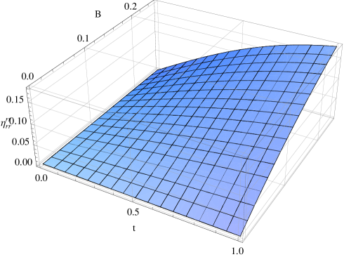
Figure 1: The $\eta^{rr}_{rr}$ viscosity coefficient as function of $B$ and $t$.

Plots of the $\eta^{r\theta}_{\theta\theta}$ viscosity coefficient are presented in Fig. (2)-Fig. (4) at different values of $B$ and $\Lambda_{0}$ as functions of $A$ and $t$ as well.

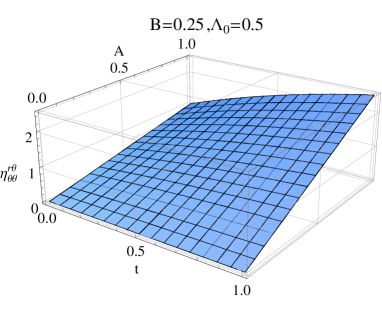
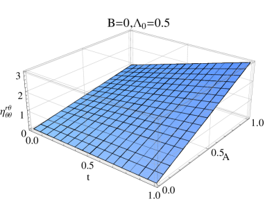
Fig. (2)-a	Fig. (2)-b

Figure 2: The $\eta^{r\theta}_{\theta\theta}$ viscosity coefficient as function of $A$ and $t$ at $\Lambda_{0}=0.5$ and different values of $B$.

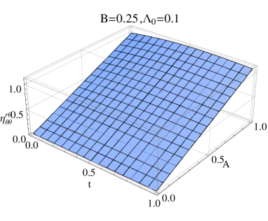
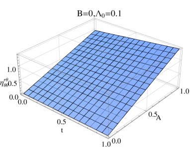
Fig. (3)-a	Fig. (3)-b

Figure 3: The $\eta^{r\theta}_{\theta\theta}$ viscosity coefficient as function of $A$ and $t$ at $\Lambda_{0}=0.1$ and different values of $B$.

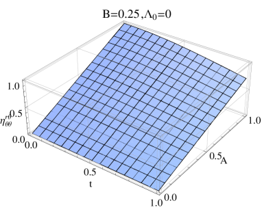
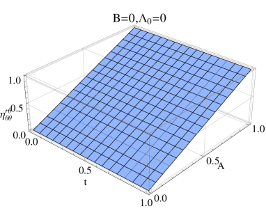
Fig. (4)-a	Fig. (4)-b

Figure 4: The $\eta^{r\theta}_{\theta\theta}$ viscosity coefficient as function of $A$ and $t$ at $\Lambda_{0}=0$ and different values of $B$.

The viscosity coefficient $\eta^{r\theta}_{r\theta}$ does not depend on $A$ and plots of this coefficient are presented as functions of $B$ at different values of $\Lambda_{0}$ in Fig. (5). For the $\Lambda_{0}\,=\,0$ case the positive value of the coefficient is taken. Parameters $\Lambda_{0}$ and $B$ are combined it such way that in the given order of the approximation the expression in the brackets in Eq. (165)-Eq. (166) remains positive for any $t$. Values of the last viscosity coefficient $\eta_{r\theta}^{rr}$ are presented in Fig. (6)-Fig. (8) as functions of $A$ and $t$ at different values of $B$ and $\Lambda_{0}$.

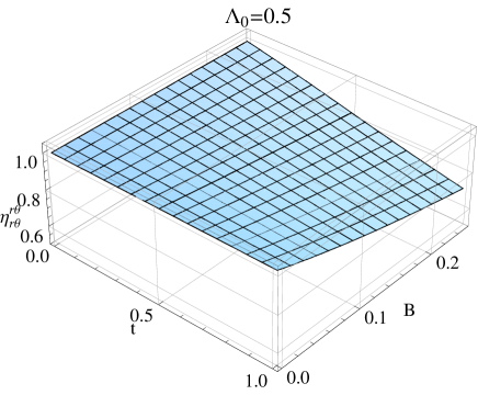
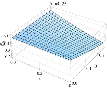
Fig. (5)-a	Fig. (5)-b
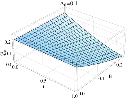
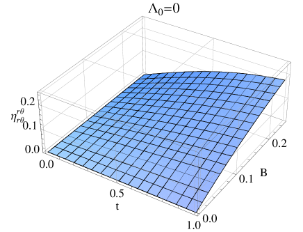
Fig. (5)-c	Fig. (5)-d

Figure 5: The $\eta^{r\theta}_{r\theta}$ viscosity coefficient as function of $B$ and $t$ at different values of $\Lambda_{0}$.

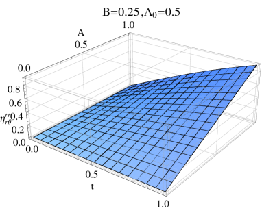
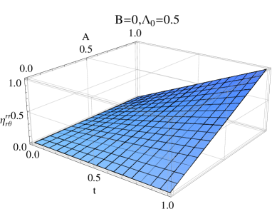
Fig. (6)-a	Fig. (6)-b

Figure 6: The $\eta^{rr}_{r\theta}$ viscosity coefficient as function of $A$ and $t$ at $\Lambda_{0}=0.5$ and different values of $B$.

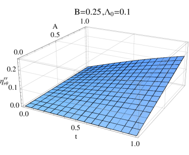
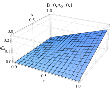
Fig. (7)-a	Fig. (7)-b

Figure 7: The $\eta^{rr}_{r\theta}$ viscosity coefficient as function of $A$ and $t$ at $\Lambda_{0}=0.1$ and different values of $B$.

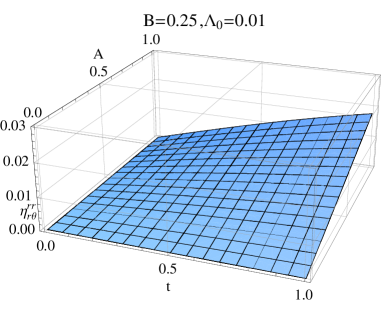
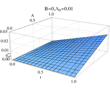
Fig. (8)-a	Fig. (8)-b

Figure 8: The $\eta^{rr}_{r\theta}$ viscosity coefficient as function of $A$ and $t$ at $\Lambda_{0}=0$ and different values of $B$.

5.2 $\Lambda_{0}\,<\,0\,$ case

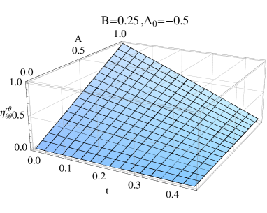
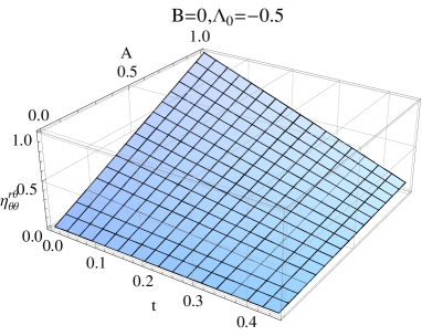
Fig. (9)-a	Fig. (9)-b

Figure 9: The $\eta^{r\theta}_{\theta\theta}$ viscosity coefficient as function of $A$ and $t$ at $\Lambda_{0}=-0.5$ and different values of $B$.

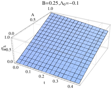
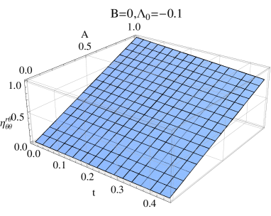
Fig. (10)-a	Fig. (10)-b

Figure 10: The $\eta^{r\theta}_{\theta\theta}$ viscosity coefficient as function of $A$ and $t$ at $\Lambda_{0}=-0.1$ and different values of $B$.

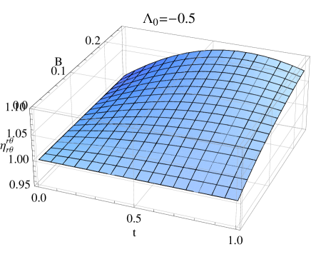
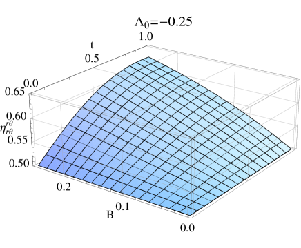
Fig. (5)-a	Fig. (5)-b
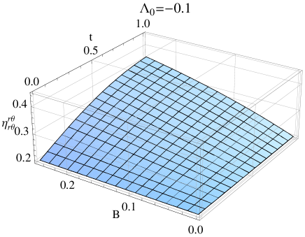
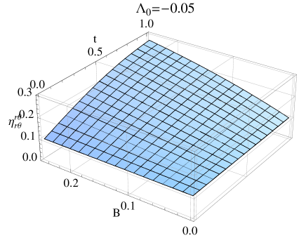
Fig. (11)-c	Fig. (11)-d

Figure 11: The $\eta^{r\theta}_{r\theta}$ viscosity coefficient as function of $B$ and $t$ at different negative values of $\Lambda_{0}$.

At the case of $\Lambda_{0}\,<\,0\,$ the only coefficients Eq. (164)-Eq. (165) are changed. Due the negative sign of $\Lambda_{0}$ in Eq. (164), time evolution of this coefficient is limited by smaller value of $t$, namely for this coefficient we have $0\,<\,t\,<\,0.45$ approximately. The plots which represent values of $\eta_{r\theta}^{\theta\theta}$ are given by Fig. (9)-Fig. (10). Finally, plots of the $\eta_{r\theta}^{r\theta}$ viscosity coefficient are presented in Fig. (11) .

6 Temperature dependence of the viscosity coefficients and quark-gluon plasma phenomenology

In order to rewrite transport coefficients Eq. (155)-Eq. (158) as functions of temperature, we introduce an effective temperature of the expanding fluid element as

$$\langle\,k\,T(t)\,\rangle_{s}^{0}\,=\,\frac{\int\,d^{3}p\,\left(H_{\bot}+H_{\|}\right)\,f_{s0}(\vec{r},\vec{v},t)}{\int\,d^{3}p\,f_{s0}(\vec{r},\vec{v},t)}\,=\,\langle\,k\,T_{\bot}(t)\,\rangle_{s}^{0}+\langle\,k\,T_{\|}(t)\,\rangle_{s}^{0}$$ (167)

with $H$ from Eq. (46):

$$H_{\bot}\,+\,H_{\|}\,=\,m\,c^{2}\,\frac{\gamma}{\beta}\,\frac{1}{2}\,\left(\,p_{r}^{2}\,+\,p_{\theta}^{2}\,\right)\,+\,\,m\,c^{2}\,p_{z}.$$ (168)

First of all, consider the $\langle\,k\,T_{\bot}(t)\,\rangle_{s}^{0}$ value. We interesting in calculation of the temperature change, i.e. we will calculate

$$\Delta\,\langle\,k\,T_{\bot}(t)\,\rangle\,=\,k\,\Delta\,\langle\,T_{\bot}(t)\,\rangle\,=\,\langle\,k\,T_{\bot}(0)\,\rangle_{s}^{0}\,-\,\langle\,k\,T_{\bot}(t)\,\rangle_{s}^{0}\,,$$ (169)

therefore we will calculate Eq. (167) taking $t\,=\,0$ limit in the end of the calculations. We have for the Eq. (167) integral:

$$\frac{\langle\,k\,T_{\bot}(t)\,\rangle_{s}^{0}\,}{m\,c^{2}}\,=\,N^{-1}\,\frac{\gamma}{2\,\beta}\,\int\,d^{3}p\,\left(\,p_{r}^{2}\,+\,p_{\theta}^{2}\,\right)\,f_{s0}(\vec{r},\,\vec{v},t)\,.$$ (170)

Using results of Eq. (96) and Eq. (109) we obtain:

$$\frac{\langle\,k\,T_{\bot}(t)\,\rangle_{s}^{0}\,}{m\,c^{2}}\, = \,\frac{1}{2}\,\left(\frac{kT_{\bot}}{mc^{2}}-\frac{\psi(r)}{mc^{2}}\right)\left(1+\frac{1+l_{0}^{2}\omega_{r}^{2}t^{2}/c^{2}}{1+t^{2}\alpha/\rho}\right)\,+\,\frac{\gamma}{2\beta}\,\left(\langle\,v_{r}\,\rangle_{s}^{0}\right)^{2}\left(1+t^{2}\frac{l_{0}^{2}\omega_{r}^{2}}{c^{2}}\right)\,-\,$$ (171)

$$- 2\,r\,t\,\frac{\gamma}{2\beta}\,\frac{l_{0}^{2}\omega_{r}^{2}}{c^{2}}\,\langle\,v_{r}\,\rangle_{s}^{0}\,+\,r^{2}\,\frac{\gamma}{2\beta}\,\frac{l_{0}^{2}\omega_{r}^{2}}{c^{2}}\,.$$

In terms of Eq. (159)-Eq. (160) definitions we rewrite Eq. (171) as :

$$\frac{\langle\,k\,T_{\bot}(t)\,\rangle_{s}^{0}\,}{m\,c^{2}}\, = \,\frac{1}{2}\,\left(\frac{kT_{\bot}}{mc^{2}}-\frac{\gamma r^{2}}{2\beta}\,B\,\left(1-\frac{t^{2}B}{1+t^{2}B}\right)\right)\left(1+\frac{1+t^{2}A^{2}}{1+t^{2}B}\right)\,+\,\frac{\gamma}{2\beta}\,\left(\langle\,v_{r}\,\rangle_{s}^{0}\right)^{2}\left(1+t^{2}A^{2}\right)\,-\,$$ (172)

$$- 2\,r\,t\,\frac{\gamma}{2\beta}\,A^{2}\,\langle\,v_{r}\,\rangle_{s}^{0}\,+\,r^{2}\,\frac{\gamma}{2\beta}\,A^{2}\,.$$

Therefore we obtain:

$$\frac{\langle\,k\,T_{\bot}(0)\,\rangle_{s}^{0}\,}{m\,c^{2}}\,=\,\left(\frac{kT_{\bot}}{mc^{2}}-\frac{\gamma r^{2}}{2\beta}\,B\,\right)\,+r^{2}\,\frac{\gamma}{2\beta}\,A^{2}\,,$$ (173)

where only linear on $\Lambda_{0}$ terms were preserved in the answer. Inserting obtained expressions in Eq. (169) we obtain:

$$\frac{\Delta\,\langle\,k\,T_{\bot}(t)\,\rangle}{mc^{2}}\, = \,\frac{1}{2}\frac{kT_{\bot}}{mc^{2}}\frac{t^{2}\left(B-A^{2}\right)}{1+t^{2}B}\,-\,\frac{\gamma r^{2}}{4\beta}\,B\,t^{2}\,\left(\frac{2B}{1+t^{2}B}\,+\,\frac{B-A^{2}}{\left(1+t^{2}B\right)^{2}}\right)\,-\,$$ (174)

$$- \frac{\gamma}{2\beta}\,\left(\left(\langle\,v_{r}\,\rangle_{s}^{01}\right)^{2}\,+\,2\,\langle\,v_{r}\,\rangle_{s}^{01}\,\langle\,v_{r}\,\rangle_{s}^{02}\,\right)\,\left(1+t^{2}A^{2}\right)\,+\,2\,r\,t\,\frac{\gamma}{2\beta}\,A^{2}\,\langle\,v_{r}\,\rangle_{s}^{01}\,.$$

We can simplify expression Eq. (174) considering only leading on $\gamma$ parameter terms:

$$\frac{\Delta\,\langle\,k\,T_{\bot}(t)\,\rangle}{mc^{2}}\,\approx\,\frac{1}{2}\frac{kT_{\bot}}{mc^{2}}\frac{t^{2}\left(B-A^{2}\right)}{1+t^{2}B}\,$$ (175)

or

$$\Delta_{\bot}\,=\,\frac{\Delta\,\langle\,T_{\bot}(t)\,\rangle}{T_{\bot}}\,\approx\,\frac{1}{2}\frac{t^{2}\left(B-A^{2}\right)}{1+t^{2}B}\,,$$ (176)

which is valid in the case of ultra-relativistic expansion of the hot spot of interest.

Second contribution into Eq. (167) integral is given by the following expression:

$$\frac{\langle\,k\,T_{\|}(t)\,\rangle_{s}^{0}\,}{m\,c^{2}}\,=\,N^{-1}\,\frac{\gamma}{2\,\beta}\,\int\,d^{3}p\,p_{z}^{2}\,f_{s0}(\vec{r},\,\vec{v},t)\,.$$ (177)

Using Eq. (88) result we obtain:

$$\frac{\langle\,k\,T_{\|}(t)\,\rangle_{s}^{0}\,}{m\,c^{2}}\,=\,\frac{\beta}{\gamma}\,+\,\Lambda_{0}\,\frac{\alpha}{\rho}\frac{r\,t\,}{\left(1\,+\,t^{2}\,\alpha/\rho\right)}\,$$ (178)

and similarly to Eq. (175) we can define:

$$\frac{\Delta\,\langle\,k\,T_{\|}(t)\,\rangle}{mc^{2}}\,=\,-\,\Lambda_{0}\,\frac{\alpha}{\rho}\frac{t\,r}{\left(1\,+\,t^{2}\,\alpha/\rho\right)}\,=\,-\,\Lambda_{0}\,\frac{t\,B}{1\,+\,t^{2}\,B}\,,$$ (179)

where we take $r\,=\,1$ as in the previous calculations. Rewriting Eq. (179) as

$$\Delta_{\|}\,=\,\frac{\Delta\,\langle\,T_{\|}(t)\,\rangle}{T_{\bot}}\,=\,-\,\Lambda_{0}\,\frac{mc^{2}}{k\,T_{\bot}}\,\frac{\alpha}{\rho}\frac{t\,r}{\left(1\,+\,t^{2}\,\alpha/\rho\right)}\,=\,-\,\Lambda_{0}\,\frac{mc^{2}}{k\,T_{\bot}}\,\frac{t\,B}{1\,+\,t^{2}\,B}\,,$$ (180)

we obtain finally

$$\Delta\,=\,\Delta_{\bot}\,+\,\Delta_{\|}\,=\,\frac{1}{2}\frac{t^{2}\left(B\,-\,A^{2}\right)}{1+\,t^{2}\,B}\,-\,\Lambda_{0}\,\frac{t\,B\,D\,}{1\,+\,t^{2}\,B}\,,$$ (181)

where

$$D\,=\,mc^{2}\,/\,k\,T_{\bot}\,>\,1\,.$$ (182)

Further we will consider only the case of an adiabatic expansion of the fluid volume when $\Lambda_{0}$ is negative.

Now, designating $\langle\,T(t\,=\,1)\,\rangle_{s}^{0}\,=\,T_{c}$ and $\langle\,T(t\,=\,0)\,\rangle_{s}^{0}\,=\,T_{0}\,=\,T_{\bot}$ we get from Eq. (181) following expression:

$$\frac{T(t\,=\,0)\,-\,T_{c}}{T(t=0)}\,=\,\frac{T_{0}\,-\,T_{c}}{T_{0}}\,=\,1\,-\,\frac{T_{c}}{T_{0}}\,=\,\frac{1}{2}\frac{B\,-\,A^{2}}{1\,+\,B}\,+\,|\Lambda_{0}|\,\frac{\,B\,D\,}{1\,+\,B}\,,$$ (183)

which allows calculate $D$ parameter on the base of known $\Lambda_{0},\,A,\,B$ parameters and $T_{c}\,/\,T_{0}$ ratio, which we also define as

$$\Delta_{1}\,=\,\,1\,-\,\frac{T_{c}}{T_{0}}\,.$$ (184)

Fixing value of $T_{0}$ we fix the value of $\Delta_{1}$. Further, basing on results of [17], we determine the maximum upper limit of initial temperature as $T_{0}^{Max}\approx\,25\,T_{c}$ that gives $\Delta_{1}^{Max}\,=\,0.96$ and determines maximum temperature range of interest as $T_{c}\,<\,T(t)\,<\,25\,T_{c}\,.$

The requested $t\,=\,t(T/T_{c})$ dependence we will obtain solving Eq. (181) together with Eq. (183):

$$1\,-\,\frac{T}{T_{0}}\,=\,1\,-\,\frac{T}{T_{c}}\,\frac{T_{c}}{T_{0}}\,=\,\frac{1}{2}\frac{t^{2}\left(B\,-\,A^{2}\right)}{1+\,t^{2}\,B}\,+\,|\Lambda_{0}|\,\frac{t\,B\,D\,}{1\,+\,t^{2}\,B}\,.$$ (185)

Inserting solution of this quadratic equation into Eq. (163)-Eq. (166) for the transport coefficients we will obtain these coefficient as function of $T\,/\,T_{c}$ ratio. Therefore, it is interesting to apply obtained formulas to the quark-gluon plasma $\eta\,/\,s$ ratio calculated in [17, 18]. In order to perform these calculations, we note that in our approach entropy is constant. Therefore, taking $s\,=\,1$, we have for the ratio of interest $\eta\,/\,s\,=\,\eta$ in dimensionless variables of the problem.

The behavior of the viscosity coefficients Eq. (163)-Eq. (166) as functions of time (temperature) is different for the each coefficient and depends on a few parameters. We assume, that among coefficients Eq. (163)-Eq. (166) the only one is not equal zero or not very small at $t\,=\,0$, whereas all other coefficients are small. In our framework, only Eq. (164) and Eq. (165) coefficients can be large enough at $t\,=\,0$ decreasing or increasing during the evolution toward some values till $t\,=\,1$. The largeness of one of them at $t\,=\,0$ requires a smallness of another and vise versa. Also, we will consider a different temperature ranges in the calculations. We will perform the calculations for $T_{0}\,=\,5\,T_{c},\,\Delta_{1}\,=\,0.8$ and for $T_{0}\,=\,25\,T_{c},\,\Delta_{1}\,=\,0.96$ temperature ranges, both of them correspond to the $t\,=\,0\,-\,1\,$ time range.

There are following different possibilities for the temperature dependence of the viscosity coefficients which we discussed above. The first one is when $\eta_{r\theta}^{\theta\theta}$ viscosity coefficient large and all other are small:

$$A\,\sim\,10^{-1}\,;\,\,A\,\gg\,B,\,\Lambda_{0}\,;\,\,B\,\simeq\,\Lambda_{0}\,.$$ (186)

Taking into account Eq. (49), Eq. (160) and assuming that

$$\omega_{r}\,\ll\,c\,/\,l_{0}\,,$$ (187)

we obtain for this combination of parameters

$$\frac{|q|\,B_{z0}}{l_{0}}\,\ll\,m\,c^{2}\,.$$ (188)

This scenario one can call a variant with small $B_{z0}$ field. The results of the calculations are presented in Fig. (12)-Fig. (13) for $\Delta_{1}\,=\,0.8\,,T_{0}\,=\,5\,T_{c}$ and $\Delta_{1}\,=\,0.96\,,T_{0}\,=\,25\,T_{c}$ values correspondingly. Due the uncertainties presented in the model we did not fit the lattice $\eta\,/\,s\,$ data in respect to our parameters obtaining instead different values of the parameters for different values of $\Delta_{1}$. The problem of more precise fixing of the parameters we discuss in the conclusion of the paper.

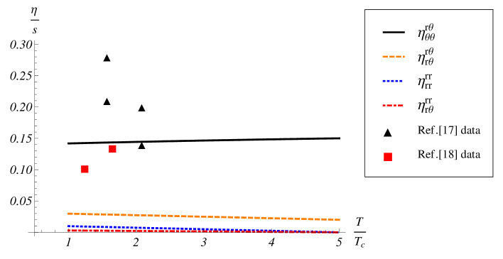
Figure 12: The $\eta\,/\,s$ ratio for the different viscosity coefficients Eq. (166)-Eq. (163) at $\Delta_{1}\,=\,0.8$, $A\,=\,0.12$, $B\,=\,0.03$ and $\Lambda_{0}\,=\,0.01$. Results of the lattice calculations for this ratio are taken from [17, 18].

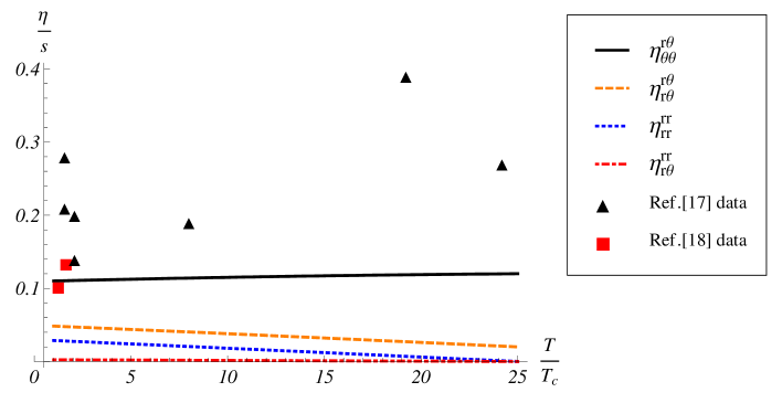
Figure 13: The $\eta\,/\,s$ ratio for the different viscosity coefficients Eq. (166)-Eq. (163) at $\Delta_{1}\,=\,0.96$, $A\,=\,0.12$, $B\,=\,0.03$ and $\Lambda_{0}\,=\,0.01$. Results of the lattice calculations for this ratio are taken from [17, 18].

We note, that in both cases of Fig. (12)-Fig. (13), parameter Eq. (182) is $\,D\,\sim\,10^{3}\,$, that is in accordance with our assumption.

Another possible restrictions on the problem’s parameters which satisfy our requests are the following:

$$\,A\,\sim\,B\,\sim\,\Lambda_{0}\,\sim\,10^{-2}\,.$$ (189)

It gives

$$\frac{|q|\,B_{z0}}{l_{0}}\,\sim\,m\,c^{2}\,$$ (190)

and therefore it can be named as variant with large $B_{z0}$ field. In this case the viscosity coefficient Eq. (165) is large at $t\,=\,0$ whereas all other coefficients remains small during the evolution. The results of the calculations with these parameter’s restrictions are presented in Fig. (14)-Fig. (15) for $\Delta_{1}\,=\,0.8\,,T_{0}^{Mac}\,=\,5\,T_{c}$ and $\Delta_{1}\,=\,0.96\,,T_{0}^{Mac}\,=\,25\,T_{c}$ values correspondingly. For these values of parameters we obtain $D\sim\,10^{2}$.

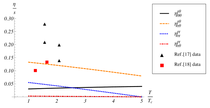
Figure 14: The $\eta\,/\,s$ ratio for the different viscosity coefficients Eq. (166)-Eq. (163) at $\Delta_{1}\,=\,0.8$, $A\,=\,0.04$, $B\,=\,0.06$ and $\Lambda_{0}\,=\,0.04$. Results of the lattice calculations for this ratio are taken from [17, 18].

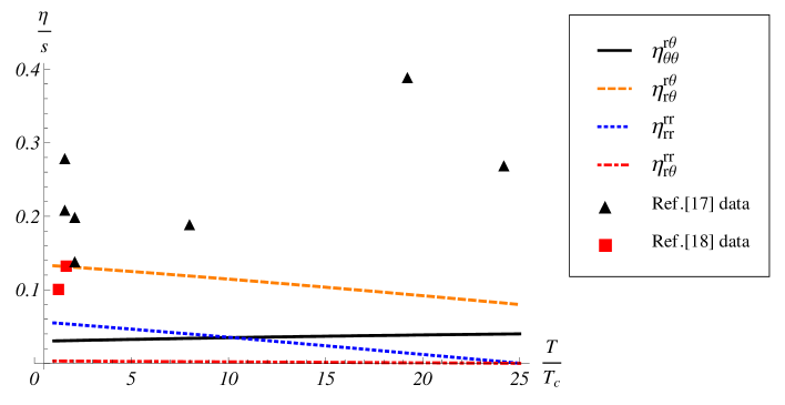
Figure 15: The $\eta\,/\,s$ ratio for the different viscosity coefficients Eq. (166)-Eq. (163) at $\Delta_{1}\,=\,0.96$, $A\,=\,0.04$, $B\,=\,0.06$ and $\Lambda_{0}\,=\,0.04$. Results of the lattice calculations for this ratio are taken from [17, 18].

The case when $\Lambda_{0}\,=\,0$, i.e. when the hot spot is neutral, we have again two different scenarios. the first one is similar to Eq. (186), whereas the second oen is given by

$$B\,\sim\,10^{-1}\,;\,\,B\,\gg\,A\,.$$ (191)

The plots for these cases are presented in Fig. (16)-Fig. (17) and Fig. (18)-Fig. (19) correspondingly for $\Delta_{1}\,=\,0.8\,,T_{0}^{Mac}\,=\,5\,T_{c}$ and $\Delta_{1}\,=\,0.96\,,T_{0}^{Mac}\,=\,25\,T_{c}$. Parameter Eq. (182) in this case does not affect on the plots, also we note that at $\,\Lambda_{0}\,=\,0$ we have $\eta^{rr}_{rr}\,=\,\eta^{r\theta}_{r\theta}$ at $\Lambda_{0}\,=\,0$.

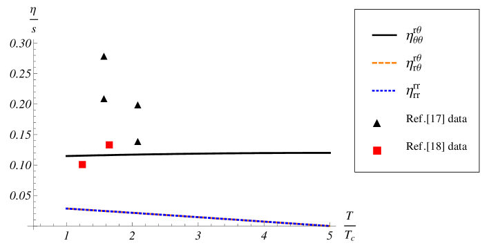
Figure 16: The $\eta\,/\,s$ ratio for the different viscosity coefficients Eq. (166)-Eq. (163) at $\Delta_{1}\,=\,0.8$, $A\,=\,0.12$, $B\,=\,0.03$ and $\Lambda_{0}\,=\,0$. Results of the lattice calculations for this ratio are taken from [17, 18].

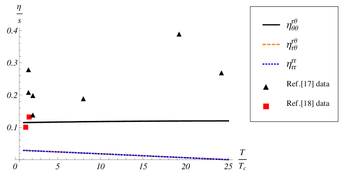
Figure 17: The $\eta\,/\,s$ ratio for the different viscosity coefficients Eq. (166)-Eq. (163) at $\Delta_{1}\,=\,0.96$, $A\,=\,0.12$, $B\,=\,0.03$ and $\Lambda_{0}\,=\,0$. Results of the lattice calculations for this ratio are taken from [17, 18].

Figure 18: The $\eta\,/\,s$ ratio for the different viscosity coefficients Eq. (166)-Eq. (163) at $\Delta_{1}\,=\,0.8$, $A\,=\,0.07$, $B\,=\,0.4$ and $\Lambda_{0}\,=\,0$. Results of the lattice calculations for this ratio are taken from [17, 18].

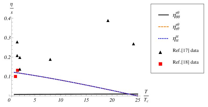
Figure 19: The $\eta\,/\,s$ ratio for the different viscosity coefficients Eq. (166)-Eq. (163) at $\Delta_{1}\,=\,0.96$, $A\,=\,0.07$, $B\,=\,0.4$ and $\Lambda_{0}\,=\,0$. Results of the lattice calculations for this ratio are taken from [17, 18].

It is worth emphasizing, that we compared results of our calculations with the [17, 18] data in order to show the importance of new degrees of freedom introduced into the model. We did not try fix the parameters precisely by the data fitting, therefore, obtained numerical values of the parameters serve as approximate restrictions which we will use in the future investigations of quark-gluon plasma phenomenological models.

7 Conclusion

In this paper we considered a model for adiabatic expansion of a small, dense, charged and rotating hot spot which was perturbed by an external electromagnetic field at the moment of time prior to the subsequent hydrodynamical evolution. The main motivation for the model’s construction was an investigation of a possibility for the small shear viscosity to entropy ratio in the system described by Vlasov’s equation. We demonstrated, that an introduction of the additional degrees of freedom in the system allows to obtain requested ratio for the expanding small volume of an ideal fluid element.

Solving perturbatively Vlasov’s equation Eq. (38) we obtained the non-equilibrium distribution function with dependence on the particular, inhomogeneous initial conditions Eq. (39) and Eq. (47). Using this function for the calculation of the momentum flux tensor we also obtained a family of the viscosity coefficients Eq. (155) - Eq. (158) whose values depend on the model’s parameters, that we consider as a main result of the manuscript. There are two such new parameters introduced in the model, initial angular velocity of the hot spot and ratio of it’s interaction with the external field to the kinetic energy at the initial moment of time. Taking these parameters to zero, we see from Eq. (155) - Eq. (158) that at the leading order the viscosity coefficients are equal to zero. Therefore, we obtained that the value of viscosity to entropy ratio is controlled by these parameters, which allow to vary this ratio correspondingly to the initial conditions of the problem, see results of Section 5, where different scenarios for the value of viscosity coefficients are described. We underline, that the shear viscosity of the bulk of QGP is result of the averaging of the independent processes of expansion of the different fluctuations immersed in some smooth and less dense surround, see [23, 24, 25, 26, 27]. The calculation of that averaged shear viscosity coefficients is a separate task, which we will consider in the subsequent publications.

In our calculations we consider the electromagnetic interactions between the particles, which are similar in the first approximation to the weakly interacting (asymptotically free) quarks and gluons inside a very small and dense initial fluctuation of the matter in the high energy scattering. Despite the fact that at high energy the interaction between relativistic particles may be very complicated, see for example [47, 48], our calculations can serve as a simple model for studying properties of the Quark-Gluon Plasma (QGP). We see from the Fig.12 - Fig.19, that in our framework, the smallness of the $\eta\,/\,s$ ratio for QGP means some restrictions on the properties of this initial fluctuation and it’s interaction with the surround. Additional restrictions in the problem are arising due the fact that we demand the smallness of all but one shear viscosity coefficients. This condition gives some additional information about microscopic structure of the system of interest. It is important to note, that even in the case of the neutral fluid element, when $\Lambda_{0}\,=\,0$, the approach allows to describe possible ranges of the $\eta\,/\,s$ ratio from [17, 18], see Fig.16 - Fig.19.

For the case of QGP, adopting the $\eta\,/\,s$ ratio from [17, 18], we obtained that the possible ranges of the values of the parameters are $A\,=\,l_{0}\,\omega_{r}\,/\,c\,\sim\,0.01\,-\,0.2$, $B\,=\,l_{0}^{2}\,\omega_{r}\,\omega_{c}\,/\,c^{2}\,-\,l_{0}^{2}\,\omega_{c}^{2}\,/\,c^{2}\,\sim\,0.01\,-\,0.4$, $\Lambda_{0}\,\sim\,0\,-\,0.04$. We see, that the value of $\Lambda_{0}$ is small in any combination, whereas the value of $\omega_{r}$ can vary rather widely. In order to fix the $\omega_{r}$ value some additional data is required therefore. Perhaps, an application of the model to the calculations of the multiplicities of the particles produced at high-energy scattering , see for example [50], can resolve this problem.

Additional perturbative corrections to our results are provided by the contributions in the next order at $\Lambda$ parameter, see Eq. (57), the present calculations were obtained in the first order to $\Lambda_{0}$ and zeroth order to $\Lambda$ perturbative parameters. Therefore, obtained results must be supplemented by the contributions to the next order in $\Lambda$ in the r.h.s. of Eq. (38). This, in turn, requires to solve Eq. (18) - Eq. (19) with the currents determined by mean velocities of Eq. (79) and Eq. (84). We will present these calculations in the subsequent publication.

Finally we conclude, that our model can be useful for the clarification of the microscopic dynamics of the interactions of asymptotically free quarks and gluons inside a QCD hot spot as well as in explaining mechanism of the shear viscosity smallness in the processes of the ideal fluid element expansion. We believe also, that the microscopic theory of the hydrodynamical expansion of the charged hot spot will provide connection between the data, obtained in high-energy collisions of protons and nuclei in the LHC and RHIC experiments [10, 11, 12, 50], and microscopic fields inside the collision region as well.

References

- [1] E.Shuryak, Nucl. Phys. B 195 111 (2009); E. Shuryak, Prog. Part. Nucl. Phys. 62, 48 (2009).
- [2] E. V. Shuryak and I. Zahed, Phys. Rev. D 70, 054507 (2004).
- [3] B. Berdnikov and K. Rajagopal, Phys. Rev. D 61, 105017 (2000).
- [4] V. Koch, A. Majumder and J. Randrup, Phys. Rev. Lett. 95, 182301 (2005).
- [5] J. Liao and E. V. Shuryak, Phys. Rev. D 73, 014509 (2006).
- [6] M. Nahrgang, C. Herold and M. Bleicher, Nucl. Phys. A904-905 2013, 899c (2013).
- [7] J. Steinheimer and J. Randrup, Phys. Rev. Lett. 109, 212301 (2012).
- [8] V. V. Skokov and D. N. Voskresensky, Nucl. Phys. A 828, 401 (2009); V. V. Skokov and D. N. Voskresensky, JETP Lett. 90, 223 (2009).
- [9] J. Randrup, Phys. Rev. C 79, 054911 (2009).
- [10] I. Arsene et al. [BRAHMS Collaboration], Nucl. Phys. A 757, 1 (2005); B. B. Back, M. D. Baker, M. Ballintijn, D. S. Barton, B. Becker, R. R. Betts, A. A. Bickley and R. Bindel et al., Nucl. Phys. A 757, 28 (2005);J. Adams et al. [STAR Collaboration], Nucl. Phys. A 757, 102 (2005); K. Adcox et al. [PHENIX Collaboration], Nucl. Phys. A 757, 184 (2005); G. Aad et al. [ATLAS Collaboration], Phys. Rev. Lett. 105, 252303 (2010); CMS Collaboration [CMS Collaboration], CMS-PAS-HIN-12-013.
- [11] P. F. Kolb, P. Huovinen, U. W. Heinz and H. Heiselberg, Phys. Lett. B 500, 232 (2001); D. Teaney, J. Lauret and E. V. Shuryak, Phys. Rev. Lett. 86, 4783 (2001).
- [12] U. W. Heinz and P. F. Kolb, Nucl. Phys. A 702, 269 (2002); A. Peshier and W. Cassing, Phys. Rev. Lett. 94, 172301 (2005).
- [13] P. Romatschke and U. Romatschke, Phys. Rev. Lett. 99, 172301 (2007); B. Schenke, S. Jeon and C. Gale, Phys. Rev. C 85, 024901 (2012).
- [14] D. Teaney, Phys. Rev. C 68, 034913 (2003).
- [15] W. Cassing and E. L. Bratkovskaya, Nucl. Phys. A 831, 215 (2009).
- [16] J. Dias de Deus, A. S. Hirsch, C. Pajares, R. P. Scharenberg and B. K. Srivastava, Eur. Phys. J. C 72, 2123 (2012); M. A. Braun, J. D. de Deus, A. S. Hirsch, C. Pajares, R. P. Scharenberg and B. K. Srivastava, arXiv:1501.01524; L. G. Gutay, A. S. Hirsch, C. Pajares, R. P. Scharenberg and B. K. Srivastava, arXiv:1504.08270.
- [17] A. Nakamura and S. Sakai, Phys. Rev. Lett. 94, 072305 (2005); S. Sakai and A. Nakamura, Lattice calculation of QGP viscosities: Present results and next project Proc. Sci. LAT2007(2007)221.
- [18] H. B. Meyer, Phys. Rev. D 76, 101701 (2007).
- [19] M. Gyulassy, D. H. Rischke and B. Zhang, Nucl. Phys. A 613, 397 (1997)
- [20] G. Torrieri, arXiv:0911.5479.
- [21] M. A. Stephanov, K. Rajagopal and E. V. Shuryak, Phys. Rev. D 60, 114028 (1999).
- [22] S. Bondarenko and K. Komoshvili, Eur. Phys. J. C 73, 2624 (2013).
- [23] R. P. G. Andrade, F. Grassi, Y. Hama, T. Kodama and W. L. Qian, Phys. Rev. Lett. 101, 112301 (2008).
- [24] G. L. Ma and X. N. Wang, Phys. Rev. Lett. 106, 162301 (2011).
- [25] R. S. Bhalerao, M. Luzum and J. Y. Ollitrault, Phys. Rev. C 84, 054901 (2011).
- [26] G. Y. Qin and B. Muller, Phys. Rev. C 85, 061901 (2012).
- [27] M. Luzum and H. Petersen, J. Phys. G 41, 063102 (2014).
- [28] L. V. Gribov, E. M. Levin and M. G. Ryskin, Phys. Rep. 100 1 (1983).
- [29] A. H. Mueller and J. Qiu, Nucl. Phys. B 268 427 (1986).
- [30] S. Bondarenko, M. Kozlov and E. Levin, Nucl. Phys. A 727, 139 (2003).
- [31] S. Bondarenko, M. Kozlov and E. Levin, Acta Phys. Polon. B 34, 3081 (2003).
- [32] S. Bondarenko, Phys. Lett. B 665, 72 (2008).
- [33] L.D.Landau, Izv. Akad. Nauk: Ser.Fiz.17, 51, (1953).
- [34] T.Epelbaum and F.Gelis, Phys. Rev. D 88, 085015 (2013).
- [35] P. B. Arnold, G. D. Moore and L. G. Yaffe, JHEP 0011, 001 (2000); P. B. Arnold, G. DMoore and L. G. Yaffe, JHEP 0305, 051 (2003).
- [36] K. Tuchin, J. Phys. G 39 025010 (2012); K. Tuchin, Adv. High Energy Phys. 2013 490495 (2013).
- [37] M. Asakawa, S. A. Bass and B. Muller, J. Phys. G 34, S839 (2007).
- [38] M. Asakawa, S. A. Bass and B. Muller, J. Phys. G 34, S839 (2007)
- [39] M. Asakawa, S. A. Bass and B. Muller, Phys. Rev. Lett. 110, no. 20, 202301 (2013).
- [40] P. Arnold, W. Florkowski, Z. Fodor, P. Foka, J. Harris, M. Lisa, H. Meyer and A. Milov et al., PoS ConfinementX , 030 (2012).
- [41] E.L.Feinberg, UFN 26, 1-30 (1983).
- [42] S. Bondarenko and K. Komoshvili, Int. J. Mod. Phys. E 24, no. 05, 1550034 (2015).
- [43] W. Cassing, V. V. Goloviznin, S. V. Molodtsov, A. M. Snigirev, V. D. Toneev, V. Voronyuk and G. M. Zinovjev, Phys. Rev. C 88, no. 6, 064909 (2013).
- [44] K. A. Lyakhov, H. J. Lee and I. N. Mishustin, Phys. Rev. C 84, 055202 (2011).
- [45] Yu.L.Klimontovich, Sov. Phys. Usp. 167, 23 (1997).
- [46] G.Kelbg, Annalen der Physik, 7 , 12 (1963); V. V. Dixit, Mod. Phys. Lett. A 5, 227 (1990); K. Dusling and C. Young, arXiv:0707.2068 [nucl-th].
- [47] L. N. Lipatov, Sov. J. Nucl. Phys. 23, 338 (1976) [Yad. Fiz. 23 (1976) 642]; E. A. Kuraev, L. N. Lipatov and V. S. Fadin, Sov. Phys. JETP 45, 199 (1977) [Zh. Eksp. Teor. Fiz. 72, 377 (1977)]; I. I. Balitsky and L. N. Lipatov, Sov. J. Nucl. Phys. 28, 822 (1978) [Yad. Fiz. 28, 1597 (1978)].
- [48] S. Bondarenko, E. Levin and J. Nyiri, Eur. Phys. J. C 25, 277 (2002).
- [49] L.Pitaevsii and E.Lifshitz, ”Physical kinetics”, Course of theoretical physics, vol.10, Butterworth-Heinemann, 2012.
- [50] D. Kharzeev, E. Levin and K. Tuchin, Phys. Rev. C 75 044903 (2007).
- [51] E. K. G. Sarkisyan and A. S. Sakharov, Eur. Phys. J. C 70 533 (2010).
- [52] V.C. Vladimirov, ”Equations of Mathematical Physics”, M.Dekker, 1971.
- [53] R.C. Davidson, ”Physics of non-neutral plasma”, WS, 2000.