Variational Limits for Phase Precision in Linear Quantum Optical Metrology

Abstract

We apply the variational method to obtain the universal and analytical lower bounds for parameter precision in some noisy systems. We first derive a lower bound for phase precision in lossy optical interferometry at non-zero temperature. Then we consider the effect of both amplitude damping and phase diffusion on phase-shift precision. At last, we extend the constant phase estimation to the case of continuous fluctuating phase estimation, and find that due to photon losses the corresponding mean square error transits from the stochastic Heisenberg limit to the stochastic standard quantum limit as the total photon flux increases.

I Introduction

A main task of quantum metrology is to find the limit of precision in the estimation of parameter $x$ qq ; uncert ; HL . According to the general quantum estimation theory, a typical parameter estimation consists in sending a probe in a suitable initial state through some phase-sensitive physical device and measuring the final state of the probe. Let $\xi$ be the outcome of the measurement, and $X(\xi)$ be the estimator of $\xi$ constructed from the outcome $x$. A local parameter precision of the estimation is quantified by the uncertainty $\delta x^{2}=\int(X(\xi)-x)^{2}p(\xi|x)d\xi$, where $p(\xi|x)$ is the conditional probability distribution of obtaining a certain outcome $\xi$ given $x$. Better precision is obtained upon decreasing $\delta x$. The minimization of $\delta x$ over all possible measurement procedures leads to the quantum Cramer-Rao inequality $\delta x\geq 1/\sqrt{\nu\mathcal{F}_{Q}}$ qq ; uncert . Here $\nu$ is the number of repeated measurements and $\mathcal{F}_{Q}$ is called the quantum Fisher information (QFI).

For quantum optical metrology with separable input states, the QFI for estimating phase $\varphi$ gives the standard quantum limit (SQL) $\delta\varphi\sim 1/\sqrt{N}$, where $N$ is the number of resources utilized in optical interferometer. In the absence of noise, employing quantum resources such as coherence and entanglement in the input state, it is possible to hit the Heisenberg limit (HL) $\delta\varphi\sim 1/N$, namely the ultimate phase estimation limit HL . In the presence of noises, it has been shown that the transition of phase precision from the HL to the SQL can occur with an increasing $N$ numer . However, for noisy systems, most of known expressions for QFI involve quite cumbersome optimization procedures when the number of resources increases. In Refs. var1 ; var2 , a general variational method is proposed to obtain a useful and analytical bound for QFI.

This variational method has been applied to phase estimation with lossy optical interferometry at zero temperature $T=0$, frequency estimation with atomic spectroscopy in the presence dephasing var1 , phase-shift estimation under phase diffusion var2 , and weak classical force estimation pure . Such obtained lower bounds could capture the main features of the corresponding numerically rigorous results, and thus provide much useful information for the ultimate limit for parameter precision.

In this paper, we apply the variational method to more noisy systems and obtain some lower bounds for parameter precision. In Section II, we first review the variational method proposed in Ref. var1 ; var2 . Then in Section III, a lower bound for phase precision in lossy optical interferometry at non-zero temperature is derived through the variational method. Next, in Section IV we consider the effect of both amplitude damping and phase diffusion on phase-shift precision. In Section V, the constant phase estimation is extended to the case of continuous fluctuating phase estimation shl , and find that the mean square error (MSE) that quantifies the estimation precision transits from the stochastic HL to the stochastic SQL as the total photon flux increases. Finally, we end with a short conclusion.

II variational method for QFI

The QFI plays a key role in quantum metrology, but the analytical expression or numerical calculation of the QFI usually pose formidable challenges, except for very specific examples when the density state can be simply put in the diagonal form exact . Recently, an alternative to find an upper bound for QFI was presented via a variational method in Refs. var1 ; var2 . This method is based on purification technique to optimize the QFI over all possible purifications of the original input state inf .

For a closed system with a pure input state $\rho_{0}=|\psi\rangle\langle\psi|$ and a unitary evolution operator $U(x)$ depending on the unknown parameter $x$, the corresponding QFI can be expressed as $\mathcal{F}_{Q}=4\Delta H^{2}$, where $\Delta H^{2}=\langle\psi|H^{2}(x)|\psi\rangle-\langle\psi|H(x)|\psi\rangle^{2}$ with $H(x)=iU^{\dagger}(x)dU(x)/dx$.

For more general situations where the input is a mixture or the evolution is not governed by a unitary operator, an analytical expression for $\mathcal{F}_{Q}$ remains an open problem. Therefore, an universal upper bound to $\mathcal{F}_{Q}$ based on the convexity of $\mathcal{F}_{Q}$ becomes necessary and can always be established for general quantum channels. If the output state $\rho_{S}(x)$ of the system is mixed, it is always possible to enlarge the size of the original Hilbert space $S$ with an auxiliary environment space $E$ and build a pure state $|\Phi_{SE}(x)\rangle$ in the enlarged space $S+E$ that satisfies $\mathrm{Tr}_{E}\rho_{SE}(x)=\rho_{S}(x)$, where $\rho_{SE}(x)=|\Phi_{SE}(x)\rangle\langle\Phi_{SE}(x)|$. The state $|\Phi_{SE}(x)\rangle$ is called a purification of $\rho_{S}(x)$.

An upper bound $C_{Q}$ of $\mathcal{F}_{Q}[\rho_{S}(x)]$ can be obtained:

$$C_{Q}=\mathcal{F}_{Q}[\rho_{SE}(x)]\geq\mathcal{F}_{Q}[\rho_{S}(x)].$$ (1)

The physical reason is that when a system plus an environment are monitored together, the acquired information on the unknown parameter can not be smaller than the information obtained when only the system is measured. It was shown in Ref. var1 that the QFI can be attainable:

$$\mathcal{F}_{Q}[\rho_{S}(x)]=\mathop{\mathrm{missing}}{min}_{|\Phi_{SE}(x)\rangle}C_{Q}[\rho_{SE}(x)].$$ (2)

Because there is always a unitary operator $u_{E}(x)$, acting only on the $E$ space, that connects two purifications $|\Psi_{SE}(x)\rangle$ and $|\Phi_{SE}(x)\rangle$ of the same state $\rho_{S}(x)$, the QFI can be found by minimizing $C_{Q}[u_{E}(x)\rho_{SE}(x)u^{\dagger}_{E}(x)]$ over all unitary operators $u_{E}(x)$ on $E$ space. The effect of $u_{E}(x)$ is to erase all non-redundant information on $x$ that has been leaked from space $S$ into the enlarged space $S+E$.

The equation for $u_{E}(x)$ optimizing $C_{Q}$ can be found by variational method,

$$h_{E}^{\mathrm{opt}}\rho_{E}+\rho_{E}h_{E}^{\mathrm{opt}}=\mathrm{Tr}_{S}\left[H_{SE}\rho_{SE}+\rho_{SE}H_{SE}\right],$$ (3)

where $\rho_{E}(x)=\mathrm{Tr}_{S}[\rho_{SE}(x)]$ is the reduced density matrix in the space $E$. Here two Hermitian operators $h_{E}$ and $H_{SE}$ are defined by

$$h_{E}=i{du^{\dagger}_{E}(x)\over dx}u_{E}(x),$$

$$i{d|\Phi_{SE}(x)\rangle\over dx}=H_{SE}(x)|\Phi_{SE}(x)\rangle.$$ (4)

After determining $u_{E}^{\mathrm{opt}}$ from Eq. (3), the QFI can be expressed as

$$\mathcal{F}_{Q}[\rho_{S}(x)]=C_{Q}[\rho_{SE}(x)]-4[\Delta h_{E}^{\mathrm{opt}}(x)]_{\Phi}^{2}.$$ (5)

Since this method is variational, whenever it is too difficult to solve Eq. (3), we can still get some non-trivial and analytical upper bounds to the QFI. The utility of this type of bounds has been exemplified with optical interferometry at $T=0$ under photon losses or phase diffusion, and atomic spectroscopy under dephasing in Refs. var1 ; var2 .

III precision limit for lossy interferometry at $T>0$

The effect of photon losses in optical interferometry at zero temperature has been thoroughly investigated in literature, but the study of the influence of temperature on phase precision is still rare. Now we apply the variational method to find an analytical lower bound for phase precision in the presence of photon losses at $T>0$.

Let the pure input state of mode $a$ be $|\psi\rangle$, and let $\rho_{S}(\varphi)$ be the mixed output state after the $\varphi$-dependent dynamical evolution. Under the photon losses and in contact with a thermal bath $E_{1}$ of mode $b$ at $T>0$, the dynamical map can described by the transformation:

$$a\to e^{-i\varphi}(a\sqrt{\eta}+b\sqrt{1-\eta}),$$ (6)

where $\eta$ quantifies the photon losses from the lossless case ($\eta=1$) to the complete absorption ($\eta=0$), and the average excitation number of the thermal bath is assumed as $\langle b^{\dagger}b\rangle=n_{T}$. To get an overall purified state, we introduce a second bath $E_{2}$ of mode $c$ and take $E_{1}$ as reduced from $E_{1}+E_{2}$ by the map: $b\to b\sqrt{n_{T}+1}+c^{\dagger}\sqrt{n_{T}}$, where both modes $b$ and $c$ are initially in the ground state. A possible purification of $\rho_{S}(\varphi)$ can thus be built with an environment with two baths $E_{1}$ and $E_{2}$. This particular purification consists of three unitary operations on the input state of $S+E_{1}+E_{2}$,

$$|\Phi_{SE}(\varphi)\rangle=U(\varphi)U_{1}U_{2}|\Phi_{0}\rangle,$$ (7)

where $U(\varphi)=e^{-i\varphi a^{\dagger}a}$, $U_{1}=e^{\theta_{1}(ab^{\dagger}-a^{\dagger}b)}$, $U_{2}=e^{\theta_{2}(b^{\dagger}c^{\dagger}-bc)}$, and $|\Phi_{0}\rangle=|\psi\rangle_{S}|0\rangle_{E_{1}}|0\rangle_{E_{2}}$ associated with $\cos\theta_{1}=\sqrt{\eta}$ and $\cosh\theta_{2}=\sqrt{n_{T}+1}$.

Any two purifications of a density matrix can be related by a unitary operator $u_{E}(\varphi)$ acting only on the environment, so we will adopt this purification as $|\Phi_{SE}(\varphi)\rangle$. The most general purification then takes the form:

$$|\Psi_{SE}(\varphi)\rangle=u_{E}(\varphi)|\Phi_{SE}(\varphi)\rangle.$$ (8)

To make the upper bound $C_{Q}$ for the QFI of the system $S$ as lower as possible, we should choose an proper $u_{E}(\varphi)$ in order to minimize the QFI of $S+E_{1}+E_{2}$. Here $u_{E}(x)$ is used to erase all non-redundant information on phase $\varphi$ that has been leaked into the environment. Noting the symmetry between $b$ and $c$, we take a trial form of $u_{E}$ to counteract the phase shift on the environment modes,

$$u_{E}(\varphi)=e^{-i\varphi[\alpha b^{\dagger}b+\beta c^{\dagger}c+\gamma(bc+b^{\dagger}c^{\dagger})]},$$ (9)

where $\alpha$, $\beta$ and $\gamma$ are adjustable variables to minimize $C_{Q}$. So this class of purifications of $\rho_{S}(\varphi)$ is given by

$$|\Psi_{SE}(\varphi)\rangle=\mathcal{U}_{SE}(\varphi)|\Phi_{0}\rangle,$$ (10)

where $\mathcal{U}_{SE}(\varphi)=u_{E}(\varphi)U(\varphi)U_{1}U_{2}$.

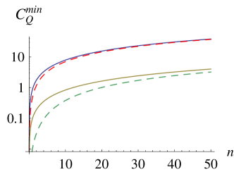
Figure 1: Comparison between the upper bound $C_{Q}^{\mathrm{min}}$ (solid lines) and the exact QFI (dashed lines) as a function of the mean energy $\langle n\rangle$ for a squeezed vacuum. Here the loss parameter is $\eta=0.8$. From bottom to top, $n_{T}=100$ and $n_{T}=10$.

The expression for $C_{Q}$ can be calculated from

$$C_{Q}=\mathcal{F}_{Q}[|\Psi_{SE}(\varphi)\rangle]=4\left[\Delta\mathcal{H}_{SE}^{2}\right]_{\Phi_{0}},$$ (11)

where

$$\mathcal{H}_{SE}(\varphi)=i\mathcal{U}_{SE}^{\dagger}(\varphi)\frac{d\mathcal{U}_{SE}(\varphi)}{d\varphi}$$ (12)

is the effective Hamiltonian in the enlarged space $S+E_{1}+E_{2}$. Using the definition of $\mathcal{U}_{SE}(\varphi)$, the explicit form of $\mathcal{H}_{SE}$ is found as

$$\mathcal{H}_{SE}=U_{2}^{\dagger}U_{1}^{\dagger}[a^{\dagger}a+\alpha b^{\dagger}b+\beta c^{\dagger}c$$

$$+\gamma(bc+b^{\dagger}c^{\dagger})]U_{1}U_{2},$$ (13)

which can be further simplified by the relations

$$U_{1}^{\dagger}\left(\begin{matrix}a\\ b\end{matrix}\right)U_{1} = \left(\begin{matrix}\cos\theta_{1}&\sin\theta_{1}\\ -\sin\theta_{1}&\cos\theta_{1}\end{matrix}\right)\left(\begin{matrix}a\\ b\end{matrix}\right),$$

$$U_{2}^{\dagger}\left(\begin{matrix}b\\ c^{\dagger}\end{matrix}\right)U_{2} = \left(\begin{matrix}\cosh\theta_{2}&\sinh\theta_{2}\\ \sinh\theta_{2}&\cosh\theta_{2}\end{matrix}\right)\left(\begin{matrix}b\\ c^{\dagger}\end{matrix}\right).$$ (14)

The final result of $C_{Q}$ is given by

$$C_{Q}=\Delta n^{2}\left(c_{1}^{2}+\alpha s_{1}^{2}\right)^{2}+{\langle n\rangle}s_{1}^{2}[c_{1}c_{2}(1-\alpha)-\gamma s_{2}]^{2}$$

$$+(\langle n\rangle+1)s_{1}^{2}[c_{1}s_{2}(1-\alpha)-\gamma c_{2}]^{2}$$

$$+[(s_{1}^{2}+\alpha c_{1}^{2}+\beta)c_{2}s_{2}+\gamma c_{1}(c_{2}^{2}+s_{2}^{2})]^{2},$$ (15)

where $\Delta n^{2}=\langle\psi|n^{2}|\psi\rangle-\langle n\rangle^{2}$, $\langle n\rangle=\langle\psi|n|\psi\rangle$ for the number operator $n=a^{\dagger}a$, and the conventions $c_{1}=\cos\theta_{1}$, $s_{1}=\sin\theta_{1}$, $c_{2}=\cosh\theta_{2}$, and $s_{2}=\sinh\theta_{2}$ are used. The minimization of $C_{Q}$ over $\alpha$, $\beta$ and $\gamma$ leads to

$$C_{Q}^{\mathrm{min}}=\frac{4}{{1\over\Delta n^{2}}+{1-\eta\over\eta}\left({n_{T}+1\over\langle n\rangle}+{n_{T}\over\langle n\rangle+1}\right)}.$$ (16)

This universal analytical upper bound to the QFI of the system allows us to evaluate the effect of temperature in the lossy interferometry irrespective of the input state. At zero temperature ($n_{T}=0$), it becomes

$$C_{Q}^{\mathrm{min}}=\frac{4}{{1\over\Delta n^{2}}+{(1-\eta)\over\eta\langle n\rangle}},$$ (17)

which is the same as the result in Ref. var1 . When the temperature goes to infinity ($n_{T}\to\infty$), Eq. (16) implies $\delta\varphi\to\infty$, i.e., no phase information can be obtained.

For the input squeezed vacuum book , $|\psi\rangle=e^{r(a^{\dagger 2}-a^{2})/2}$ with $\langle n\rangle=\sinh^{2}r$ and $\Delta n^{2}=2\langle n\rangle(\langle n\rangle+1)$, the exact QFI can be obtained by me

$$\mathcal{F}_{Q}[\rho_{S}(\varphi)]=\frac{4u^{2}}{1+v^{2}-u^{2}},$$ (18)

where $u=\eta\sinh 2r$ and $v=\eta\cosh 2r+(1-\eta)(2n_{T}+1)$. The comparison of $C_{Q}^{\mathrm{min}}$ with this exact QFI is shown in Fig. 1. It can be seen that the higher the temperature is, the worse the phase precision is. We can also see that the variational bound saturates the exact QFI as $\langle n\rangle\to\infty$.

IV precision limit under damping and diffusion

Besides photon losses, phase diffusion is another important source of noise in optical phase estimation and should be taken into account. A numerical study of the influence of phase diffusion on the optimal phase precision was presented in Ref. dephase . Then an analytical lower bound was found by the above variational method in Ref. var2 . However, the effect of photon losses is not considered at the same time. In this section, we will discuss the effect of both photon losses and phase diffusion on the limit of phase precision.

For simplicity, suppose a pure input state $|\psi\rangle$ of mode $a$, which undergoes a phase shift $\varphi$ due to some physical process. In the presence of photon losses and phase diffusion, a specific purification of the output state $\rho_{S}(\varphi)$ is

$$|\Phi_{SE}(\varphi)\rangle=U(\varphi)U_{\theta}U_{\lambda}|\Phi_{0}\rangle,$$ (19)

where $U_{\theta}=e^{\theta(ab^{\dagger}-a^{\dagger}b)}$ and $U_{\lambda}=e^{i(2\lambda)a^{\dagger}ax_{2}}$ with $\cos\theta=\sqrt{\eta}$, $x_{2}=(c+c^{\dagger})/\sqrt{2}$, and $\lambda$ characterizes the strength of phase diffusion in the process

$$\rho_{S}\to\frac{1}{\sqrt{4\pi\lambda^{2}}}\int e^{-{\phi^{2}\over 4\lambda^{2}}}U^{\dagger}(\phi)\rho_{S}U(\phi)d\phi.$$ (20)

In terms of the Fock basis of the system, the action of phase diffusion takes

$$|l\rangle\langle k|\to e^{-\lambda^{2}(k-l)^{2}}|l\rangle\langle k|.$$ (21)

In order to get a tighter upper bound to $\mathcal{F}_{Q}[\rho_{S}(\varphi)]$, we take a trial form of $u_{E}(\varphi)$ inspired by Ref. var2 ,

$$u_{E}(\varphi)=e^{-i\alpha\varphi b^{\dagger}b+i\beta\varphi p_{2}/(2\lambda)}.$$ (22)

This choice of $u_{E}(\varphi)$ leads to $C_{Q}=4[\Delta\mathcal{H}_{SE}^{2}]_{\Phi_{0}}$, where $\mathcal{H}_{SE}=U^{\dagger}_{\lambda}U^{\dagger}_{\theta}[a^{\dagger}a+\alpha b^{\dagger}b-\beta p_{2}/(2\lambda)]U_{\theta}U_{\lambda}$ with $p_{2}=(c-c^{\dagger})/(i\sqrt{2})$. Using the identity (14) and $U^{\dagger}_{\lambda}p_{2}U_{\lambda}=p_{2}+2\lambda a^{\dagger}a$, we have

$$C_{Q}=4\Delta n^{2}[\eta+\alpha(1-\eta)-\beta]^{2}$$

$$+4\langle n\rangle(1-\alpha)^{2}\eta(1-\eta)+\frac{\beta^{2}}{2\lambda^{2}}.$$ (23)

The minimization of $C_{Q}$ over the variables $\alpha$ and $\beta$ gives

$$C_{Q}^{\mathrm{min}}=\frac{4}{\frac{1}{\Delta n^{2}}+{(1-\eta)\over\eta\langle n\rangle}+8\lambda^{2}}.$$ (24)

For $\eta=1$, it gives $\delta\varphi^{2}\geq 1/(4\Delta n^{2})+2\lambda^{2}$, which is the same as the result in Ref. var2 .

Following the steps in Section III, we can also include the effect of temperature during the process of photon losses. Through some calculations, we obtain the phase precision

$$\delta\varphi^{2}\geq{1\over 4\Delta n^{2}}+{1-\eta\over 4\eta}\left({n_{T}+1\over\langle n\rangle}+{n_{T}\over\langle n\rangle+1}\right)+2\lambda^{2}.$$ (25)

The presence of a constant term in this equation means that phase diffusion is usually more harmful to phase precision than photon losses.

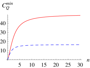
Figure 2: Comparison between the upper bound $C_{Q}^{\mathrm{min}}$ (solid lines) and the lower bound $\mathcal{I}_{Q}^{\mathrm{opt}}$ (dashed lines) as a function of the mean energy $\langle n\rangle$ for a squeezed vacuum. Here the loss parameter and diffusion strength are $\eta=0.95$ and $\lambda=0.1$, respectively. The temperature is set to zero.

For the input squeezed vacuum, the exact QFI is not known analytically. Instead, a lower bound $\mathcal{I}_{M}$ of the QFI can be deduced from the measurement $M=i(a^{2}-a^{\dagger 2})$ me . It gives

$$\mathcal{I}_{M}=\frac{|\partial_{\varphi}\langle M\rangle_{\rho_{S}}|^{2}}{[\Delta M^{2}]_{\rho_{S}}},$$ (26)

where $\langle M\rangle_{\rho_{S}}=ue^{-4\lambda^{2}}\sin(2\varphi)$ and

$${[\Delta M^{2}]_{\rho_{S}}} = 1+v^{2}+{u^{2}\over 2}[1+e^{-8\lambda^{2}}$$ (27)

$$-e^{-8\lambda^{2}}(1+3e^{-8\lambda^{2}})\cos(4\varphi)].$$

The optimization of $\mathcal{I}_{M}$ over $\varphi$ corresponds to $\varphi=0$, and

$$\mathcal{I}_{M}^{\mathrm{opt}}=\frac{4u^{2}e^{-8\lambda^{2}}}{1+v^{2}+{u^{2}}(1-3e^{-8\lambda^{2}})/2}.$$ (28)

The comparison of $C_{Q}^{\mathrm{min}}$ in Eq. (25) with $\mathcal{I}_{M}^{\mathrm{opt}}$ is plotted in Fig. 2. We see that the upper bound $C_{Q}^{\mathrm{min}}$ to the QFI is always larger than its lower bound $\mathcal{I}_{M}^{\mathrm{opt}}$ and the exact QFI should lay between them. It also displays that both of bounds approaches to some constant value as the total available energy go to infinity.

V point estimation precision limit for a continuous fluctuating phase

In the case of estimating a constant phase, the fundamental bound to phase precision is the HL, which is a quadratic improvement over the SQL. Contrary to this constant situation, the fundamental bound to estimating Wiener phase fluctuations $\varphi(t)$ with a beam $a(t)$ (obeying $[a(t),a^{\dagger}(t^{\prime})]=\delta(t-t^{\prime})$) is the stochastic HL, which shows a MSE scaling as $\mathcal{N}^{-2/3}$, while the stochastic SQL scales as $\mathcal{N}^{-1/2}$ shl . Here the beam is assumed as Gaussian stationary statistics, and $\mathcal{N}=\langle a^{\dagger}(t)a(t)\rangle$ is the mean flux (photons per second) in the beam. In this section, we will show a transitive behavior of MSE scaling from the stochastic HL to the stochastic SQL as the beam undergoing some photon losses.

In Ref. defer , a continuous form of the quantum Cramer-Rao inequality was derived, giving a lower bound on the MSE of any unbiased estimator $\hat{\varphi}(t)$, of a time-varying phase $\hat{\varphi}(t)$,

$$\langle[\hat{\varphi}(t)-\varphi(t)]^{2}\rangle\geq\mathcal{F}^{-1}(t,t).$$ (29)

Here $\mathcal{F}(t,t^{\prime})$ is the Fisher information matrix (with continuous indices $t$ and $t^{\prime}$) of the phase of the beam. It includes the sum of quantum and classical parts $\mathcal{F}(t,t^{\prime})=\mathcal{F}_{Q}(t,t^{\prime})+\mathcal{F}_{C}(t,t^{\prime})$. The (matrix) inverse in Eq. (29) is defined by $\int\mathcal{F}^{-1}(t,s)\mathcal{F}(s,t^{\prime})ds=\delta(t-t^{\prime})$. Because the beam is stationary, all quantities dependent on two times $t$ and $t^{\prime}$ are only functions of $t-t^{\prime}$.

In order to determine $\mathcal{F}^{-1}(0)$, put Eq. (3) into Eq. (4) and take the Fourier transform, to give be

$$\tilde{\mathcal{F}}^{-1}(\omega)={1\over\tilde{\mathcal{F}}_{Q}(\omega)+\tilde{\mathcal{F}}_{C}(\omega)}$$ (30)

for the Fourier transform of $\mathcal{F}^{-1}(t-t^{\prime})$. The value of $\mathcal{F}^{-1}(0)$ is then given by

$$\mathcal{F}^{-1}(0)=\frac{1}{2\pi}\int{1\over\tilde{\mathcal{F}}_{Q}(\omega)+\tilde{\mathcal{F}}_{C}(\omega)}d\omega.$$ (31)

In Refs. shl , an upper bound to $\mathcal{F}_{Q}(t,t^{\prime})$ is taken as $4\langle\Delta n(t)\Delta n(t^{\prime})\rangle$, corresponding to the lossless case, and the Wiener phase spectrum $\tilde{\mathcal{F}}_{C}(\omega)=\kappa^{p-1}/|\omega|^{p}$ ($p>1$) is assumed. Considering the analytical properties of $\tilde{\mathcal{F}}_{Q}(\omega)$ for the stationary Gaussian beam, it was shown that the MSE scales as $\mathcal{N}^{2(p-1)/(p+1)}$.

However, when the beam suffers some photon losses, the above lower bound to the MSE is not tight. Similar to the case of constant phase, we introduce an vacuum environment $b(t)$ (obeying $[b(t),b^{\dagger}(t^{\prime})]=\delta(t-t^{\prime})$ and $\langle b^{\dagger}(t)b(t)\rangle=0$) to purify the mixed output state. This vacuum is coupled with the beam through the unitary operator $U_{\theta}=\exp\left[\theta\int[a(t)b^{\dagger}(t)-a^{\dagger}(t)b(t)]dt\right]$ with $\cos\theta=\sqrt{\eta}$. To find a upper bound $C_{Q}(t,t^{\prime})$ of $\mathcal{F}_{Q}(t,t^{\prime})$, we apply a variational unitary operator $\exp[-i\beta\int\varphi(t)b^{\dagger}(t)b(t)dt]$ on the purified state with $\beta$ as a variational parameter. The total transformation is thus given by

$$\mathcal{U}_{SE}=\exp\left[-i\int\varphi(t)[a^{\dagger}(t)a(t)+\beta b^{\dagger}(t)b(t)]dt\right]U_{\theta},$$ (32)

and the upper bound to $\mathcal{F}_{Q}(t,t^{\prime})$ follows

$$C_{Q}(t,t^{\prime})=4\langle\Delta n(t)\Delta n(t^{\prime})\rangle[\eta+\beta(1-\eta)]^{2}$$

$$+4\mathcal{N}\delta(t-t^{\prime})(1-\beta)^{2}\eta(1-\eta).$$ (33)

Since $\beta$ is arbitrary, we set $\beta=\eta/(\eta-1)$ and $C_{Q}$ becomes

$$C_{Q}={4\eta\mathcal{N}\over(1-\eta)}\delta(t-t^{\prime}).$$ (34)

This implies that

$$\mathcal{F}^{-1}(0) \geq {1\over 2\pi}\int_{-\infty}^{\infty}\frac{\kappa^{p-1}}{|\omega|^{p}+\kappa^{p-1}{4\eta\mathcal{N}\over(1-\eta)}}d\omega$$ (35)

$$= \mathcal{O}\left((\mathcal{N}/\kappa)^{1-p\over p}\right),$$

which is just the stochastic SQL. In other words, in presence of photon losses, the special quantum strategy to estimate a fluctuating phase does not provide an order of magnitude improvement with respect to the standard light beams.

To illustrate the transitive behavior of the MSE scaling, we use the analytical property of the Fourier transform of $\langle\Delta n(t)\Delta n(t^{\prime})\rangle$ under the same conditions as in Refs. shl , and find that

$$\mathcal{F}^{-1}(0) \geq \mathop{\max_{\left\{\beta\right\}}}{1\over 2\pi}\int_{-\infty}^{\infty}\frac{\kappa^{p-1}}{|\omega|^{p}+\kappa^{p-1}\tilde{C}_{Q}(\omega)}d\omega$$

$$\geq {1\over\pi}\int_{L}^{\infty}\frac{\kappa^{p-1}}{\omega^{p}+D}d\omega$$

$$\geq {1\over\pi}\int_{0}^{\infty}\frac{\kappa^{p-1}}{\omega^{p}+D}d\omega-{1\over\pi}\int_{0}^{L}\frac{\kappa^{p-1}}{D}d\omega$$

$$\geq \mathcal{O}(D^{{1-p\over p}}),$$ (37)

where the inequality in the last line holds for $L\leq\mathcal{O}(D^{1/p})$. Here $\mu$ is an arbitrary positive constant, $L=8\pi\mathcal{N}^{2}/\mu$, and

$$D={4\kappa^{p-1}\eta\mathcal{N}(17\mathcal{N}+4\mu)\over\mathcal{N}(17-\eta)+4\mu(1-\eta)}$$ (38)

is obtained by minimizing the denominator over $\beta$.

To get a tighter bound on $\mathcal{F}^{-1}(0)$ we should take $\mu$ as small as possible under the condition $L\leq\mathcal{O}(D^{1/p})$. For the lossless case $\eta=1$, $\mu=\Theta(\mathcal{N}^{\frac{2p}{p+1}})$. For the lossy case $\eta<1$, $\mu=\Theta(\mathcal{N}^{2-\frac{1}{p}})$. These values of $\mu$ lead to

$$\mathcal{F}^{-1}(0)\geq{\bigg{\{}}\begin{matrix}\mathcal{O}\left((\mathcal{N}/\kappa)^{2(1-p)\over p+1}\right),\quad\ \rm{for}\quad\ \eta=1,\\ \mathcal{O}\left((\mathcal{N}/\kappa)^{1-p\over p}\right),\quad\ \rm{for}\quad\ \eta<1\end{matrix}$$ (39)

in the large $\mathcal{N}$ limit.

Next we use a particular example to demonstrate the above results in details. In the squeezing vacuum model in Ref. scien , a phase fluctuation is modeled by the spectrum $\tilde{\mathcal{F}}_{C}(\omega)=\kappa/(\lambda^{2}+\omega^{2})$, which is asymptotically identical to the Wiener phase spectrum ($p=2$). For this beam, the Fourier transform of $\Sigma(t-t^{\prime})=4\langle\Delta n(t)\Delta n(t^{\prime})\rangle$ yields

$$\tilde{\Sigma}(\omega) = 4\mathcal{N}+\frac{\gamma^{3}}{16}\bigg{[}\frac{(R_{+}-1)^{2}(1-x)^{3}}{(1-x)^{2}\gamma^{2}+\omega^{2}}$$ (40)

$$+\frac{(R_{-}-1)^{2}(1+x)^{3}}{(1+x)^{2}\gamma^{2}+\omega^{2}}\bigg{]},$$

where the total photon flux is given by

$$\mathcal{N}=\frac{\gamma}{16}\left[(R_{+}-1)(1-x)+(R_{-}-1)(1+x)\right].$$ (41)

For an optical parameter oscillator, $R_{\pm}$ (for a squeezed vacuum $R_{+}R_{-}=1$) are the anti-squeezing and squeezing levels at the center frequency, respectively. Here $\gamma$ is the cavity’s decay rate and $x=(\sqrt{R_{+}}-1)/(\sqrt{R_{+}}+1)$ is the normalized pump amplitude.

To fulfil the numerical calculation, we take $\kappa=\lambda=1$ and $R_{+}=1/R_{-}=16\mathcal{N}^{1/3}$. The value of $\gamma$ is solved by Eq. (41). Putting all equations together and performing the integral, the final results after optimizing over $\beta$ are shown in Fig. 3. It can be seen that the presence of photon losses always blur the MSE and make a transitive behavior of the MSE from the stochastic HL scaling $\mathcal{N}^{-2/3}$ to the stochastic SQL scaling $\mathcal{N}^{-1/2}$ as the total photon flux increases.

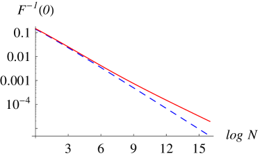
Figure 3: The plot of the upper bound to $\mathcal{F}^{-1}(0)$ with respect to the total photon flux $\mathcal{N}$ for the squeezed vacuum model in Ref. scien . The solid (dashed) line denotes the result for the lossy (lossless) case. Here $\eta=0.95$.

VI Conclusion

In summary, we have applied the variational method to obtain the universal and analytical lower bounds for phase precision in some noisy systems. We have derived a lower bound for phase precision in lossy optical interferometry at non-zero temperature that allows us to evaluate the effect of temperature on phase estimation. We have also discussed the effect of both amplitude damping and phase diffusion on phase-shift precision, which approaches to a constant term even when the total available energy goes to infinity. At last, we have extended the constant phase estimation to the case of continuous fluctuating phase estimation, and have found that due to photon losses the corresponding MSE transits from the stochastic HL to the stochastic SQL as the total photon flux increases.

References

• (1) C.Β W. Helstrom, Quantum Detection and Estimation Theory (Academic Press, New York, 1976).
• (2) S.Β L. Braunstein and C.Β M. Caves, Phys. Rev. Lett. 72, 3439 (1994).
• (3) V.Β Giovannetti, S.Β Lloyd, and L.Β Maccone, Phys. Rev. Lett. 96, 010401 (2006).
• (4) U. Dorner, et al., Phys. Rev. Lett. 102, 040403 (2009).
• (5) B. M. Escher, R. L. de Matos Filho, and L. Davidovich, Nature Physics 7, 406 (2011).
• (6) B. M. Escher, L. Davidovich, N. Zagury, and R. L. de Matos Filho, Phys. Rev. Lett. 109, 190404 (2012).
• (7) C. L. Latune, B. M. Escher, R. L. de Matos Filho, and L. Davidovich, Phys. Rev. A 88, 042112 (2013).
• (8) D. W. Berry, M. J. W. Hall, and H. M. Wiseman Phys. Rev. Lett. 111, 113601 (2013); D. W. Berry, M. Tsang, M. J. W. Hall, and H. M. Wiseman, Phys. Rev. X 5, 031018 (2015)
• (9) A. Monras and M.G.A. Paris, Phys. Rev. Lett. 98, 160401 (2007); M. Aspachs, G. Adesso, and I. Fuentes, Phys. Rev. Lett. 105, 151301 (2010); Y.M. Zhang, X.W. Li, W. Yang, and G.R. Jin, Phys. Rev. A 88, 043832. (2013).
• (10) M.Β A. Nielson and I.Β L. Chuang, Quantum Information and Computation (Cambridge University Press, Cambridge, 2000).
• (11) D.Β F. Walls and G.Β J. Milburn, Quantum Optics (Springer-Verlag, 1994).
• (12) Y. Gao and H. Lee, Euro. Phys. J. D 68, 347 (2014).
• (13) Marco G. Genoni, Stefano Olivares, and Matteo G. A. Paris, Phys. Rev. Lett 106, 153603 (2011)
• (14) M. Tsang, H.Β M. Wiseman, and C.Β M. Caves, Phys. Rev. Lett. 100, 073601 (2011).
• (15) H. Yonezawa et al., Science 337, 1514 (1994).