Phase diagram of a bidispersed hard rod lattice gas in two dimensions

Abstract

We obtain, using extensive Monte Carlo simulations, virial expansion and a high-density perturbation expansion about the fully packed monodispersed phase, the phase diagram of a system of bidispersed hard rods on a square lattice. We show numerically that when the length of the longer rods is $7$, two continuous transitions may exist as the density of the longer rods in increased, keeping the density of shorter rods fixed: first from a low-density isotropic phase to a nematic phase, and second from the nematic to a high-density isotropic phase. The difference between the critical densities of the two transitions decreases to zero at a critical density of the shorter rods such that the fully packed phase is disordered for any composition. When both the rod lengths are larger than $6$, we observe the existence of two transitions along the fully packed line as the composition is varied. Low-density virial expansion, truncated at second virial coefficient, reproduces features of the first transition. By developing a high-density perturbation expansion, we show that when one of the rods is long enough, there will be at least two isotropic-nematic transitions along the fully packed line as the composition is varied.

Statistical mechanics of model systems (Ising model, Potts model, field-theory models, Monte Carlo techniques, etc.) Lattice theory and statistics (Ising, Potts, etc.) Theory and modeling of specific liquid crystal transitions, including computer simulation

1 Introduction

Entropy-driven transitions in systems of rod-like particles have long been an active area of theoretical and experimental research. Experimental realizations of such systems include tobacco mosaic virus [1], $fd$ virus [2, 3, 4], silica colloids [5, 6], boehmite particles [7, 8], DNA origami nanoneedles [9], liquid crystals [10] and adsorbed gas molecules on metal surfaces [11, 12, 13, 14, 15]. A system of hard sphero-cylinders in three-dimensional continuum undergoes a transition from an isotropic phase to an orientationally ordered nematic phase as density is increased. Further increase in density leads to a smectic phase with partial translational order and a solid phase [16, 18, 19, 17, 20, 10]. In two-dimensional continuum, a Kosterlitz-Thouless transition to a high-density phase with power law correlations may be observed [21, 22, 23, 24]. Lattice models of hard rods, of interest to this paper, also have a rich phase diagram in two dimensions, while not much is known in three dimensions.

Consider monodispersed hard rods on a two-dimensional lattice, where each rod occupies $k$ consecutive lattice sites along any of the lattice directions and no two rods may overlap. When $k=2$ (dimers), the system is known to be disordered at all densities [28, 27, 26, 25]. When $k\geq 7$, there are, interestingly, two transitions: first, from a low-density disordered to an intermediate density nematic phase and second, from the nematic to a high-density disordered phase [29, 30]. While the first transition belongs to the Ising (three state Potts) universality class for the square (triangular) lattice [31], the universality class of the second transition remains unclear with the numerically obtained critical exponents differing from those of the first transition, though a crossover to the Ising exponents at larger length scales could not be ruled out [30, 32]. Exact analysis, restricted to a rigorous proof for existence of the first transition when $k\gg 1$ [33] and exact solution on a Bethe-like lattice [34] does not shed any light on the second transition. The fully packed limit of monodispersed rods is disordered and may be mapped onto a height model with a $k-1$ dimensional height field, showing that orientation-orientation correlations decay as a power law [25, 35, 36].

Polydispersity in length of the particles is hardly avoidable in experiments and results in features such as strong fractionation, two distinct nematic phases and nematic-nematic or isotropic-nematic-nematic phase coexistence [7, 8]. Some of these features may be obtained using density functional theory, virial expansion or Monte Carlo simulations in the continuum [40, 41, 42, 37, 38, 39, 43, 44, 45, 46]. The lattice counterpart is less studied and the phase diagram is mostly unexplored. A particular model of polydispersed rods with a rod of length $k$ having a weight $z_{e}^{2}z_{i}^{k-2}$, where $z_{i}$ ($z_{e}$) is the fugacity of an internal (endpoint) monomer was shown to undergo an isotropic-nematic transition using transfer matrix methods [47]. When $z_{e}=\sqrt{z_{i}/2}$, the model may solved exactly by mapping it to the two-dimensional Ising model [48]. A second transition to the high-density disordered phase is absent [47]. However, in this model, densities of different species cannot be changed independently.

What is the phase diagram for lattice models of polydispersed rods? Does polydispersity preserve the second phase transition into a high-density disordered phase? Is the fully packed line still disordered or could there be regions with nematic order? In this letter, we address these questions by determining the phase diagram of bidispersed 2-7, 6-7, and 7-8 mixtures using extensive Monte Carlo simulations and studying generic bidispersed mixtures using low-density virial expansions and high-density perturbation expansions close to full packing. In particular, we show that the second transition at high densities persists, and if one of the rod lengths is large enough, the system at full packing will exhibit at least two isotropic-nematic transitions as the ratio of densities of the two species is varied.

2 Model and the Monte Carlo algorithm

Consider a bidispersed system of rods of length $k_{1}$ and $k_{2}$ on a square lattice of size $V=L\times L$ with periodic boundary conditions, where each rod is either horizontal or vertical. A horizontal (vertical) rod of length $k_{i}$ (where $i=1,2$) occupies $k_{i}$ consecutive lattice sites along the $x$ ($y$)-axis. No two rods are allowed to intersect or equivalently, each site may be occupied by utmost one rod. A fugacity $z_{k_{i}}=e^{\mu_{k_{i}}}$ is associated with each rod of length $k_{i}$, $i=1,2$, where $\mu_{k_{i}}$ is the corresponding reduced chemical potential.

We simulate this model using a constant fugacity grand canonical Monte Carlo algorithm involving cluster moves. For fixed fugacities $z_{k_{1}}$ and $z_{k_{2}}$, the system reaches an equilibrium density $\rho(z_{k_{1}},z_{k_{2}})$, defined as the fraction of sites occupied by the rods. This algorithm is an adaptation of the scheme that was quite efficient in equilibrating systems of monodispersed long rods [49, 30]. Variants of this algorithm have been used to study systems of hard rectangles [50, 51, 52], disks on square lattice [53] and mixtures of squares and dimers [55]. We briefly discuss the algorithm here.

Choose at random a row or column of the lattice. If a row is chosen, all the horizontal rods on that row are removed, while the rest of the configuration is kept unchanged. The row now consists of intervals of empty sites separated by the sites occupied by vertical rods. These empty intervals are re-occupied with a new configuration of horizontal rods consistent with equilibrium probabilities. If, instead of a row, a column is chosen, a similar evaporation-deposition operation is done with vertical rods. The calculation of these equilibrium probabilities reduces to a one-dimensional problem.

Let $\Omega_{o}(z_{k_{1}},z_{k_{2}};\ell)$ be the grand canonical partition function of a one-dimensional chain of length $\ell$ with open boundary conditions. The probability that the first site of the one-dimensional chain is occupied by the left-most site of a rod of length $k_{i}$ is $p^{\ell}_{i}=z_{i}\Omega_{o}(z_{k_{1}},z_{k_{2}};\ell-k_{i})/\Omega_{o}(z_{k_{1}},z_{k_{2}};\ell)$, where $i=1,2$. The partition functions $\Omega_{o}(z_{k_{1}},z_{k_{2}};\ell)$ obeys the recursion relation $\Omega_{o}(z_{k_{1}},z_{k_{2}};\ell)=\sum_{i=1}^{2}z_{k_{i}}\Omega_{o}(z_{k_{1}},z_{k_{2}};\ell-k_{i})+\Omega_{o}(z_{k_{1}},z_{k_{2}};\ell-1)$ for $\ell\geq\min(k_{1},k_{2})$, with the boundary conditions $\Omega_{o}(z_{k_{1}},z_{k_{2}};\ell)=1$ for $\ell=0,1,\dots,\min(k_{1},k_{2})-1$ and $\Omega_{o}(z_{k_{1}},z_{k_{2}};\ell)=0$ for $\ell<0$. The partition function of a one-dimensional chain of length $\ell$ with periodic boundary condition, $\Omega_{p}(z_{k_{1}},z_{k_{2}};\ell)$, is easy to determine once $\Omega_{o}(z_{k_{1}},z_{k_{2}};\ell)$ is known. It obeys the recursion relation $\Omega_{p}(z_{k_{1}},z_{k_{2}};\ell)=\sum_{i=1}^{2}z_{k_{i}}k_{i}\Omega_{o}(z_{k_{1}},z_{k_{2}};\ell-k_{i})+\Omega_{o}(\ell-1)$. The recursion relations may be solved exactly for $\Omega_{o}(z_{k_{1}},z_{k_{2}};\ell)$ and $\Omega_{p}(z_{k_{1}},z_{k_{2}};\ell)$. The list of relevant probabilities ${p^{\ell}_{i}}$ for all $\ell\leq L$ are stored in order to reduce computational time.

In addition to the evaporation-deposition moves, we also implement a flip move [50]. We choose a site at random. Only if it is the bottom-left corner of a block of size $(k_{i}\times k_{i})$ containing $k_{i}$ aligned parallel horizontal (vertical) rods, it is replaced by a similar block of $k_{i}$ vertical (horizontal) rods. One Monte Carlo (MC) move contains $2L$ evaporation-deposition moves and $L^{2}$ flip moves. All the numerical results presented in this paper are obtained using a parallelized version of the algorithm.

The largest system size that we simulate is $L=560$. A single data point in the phase diagrams (total of 47 data points), has been obtained using (on an average) 30 runs of Monte Carlo simulation.

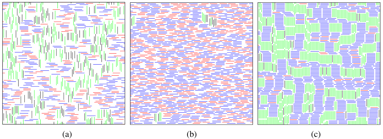
Figure 1: Snapshots of the system when $k_{1}=7$ and $k_{2}=8$ at (a) low-density isotropic (I) phase where $\rho_{7}\approx 0.187$ and $\rho_{8}\approx 0.311$ ($\mu_{7}=-2.0$, $\mu_{8}=-1.4$), (b) intermediate density nematic (N) phase where $\rho_{7}\approx 0.372$ and $\rho_{8}\approx 0.441$ ($\mu_{7}=1.5$, $\mu_{8}=2.0$) and (c) high-density isotropic (I) phase where $\rho_{7}\approx 0.055$ and $\rho_{8}\approx 0.922$ ($\mu_{7}=7.2$, $\mu_{8}=11.0$). The horizontal and vertical rods of length $7$ are colored red and black, and the same of length $8$ are colored blue and green respectively.

3 Results

We study three different mixtures: 2-7, 6-7, and 7-8. These choices were made for the following reasons. A monodispersed system of hard rods shows phase transition only when the rod length $k\geq 7$. Rods of length $2$ and $6$ being the smallest and largest lengths that do not show a nematic phase, studying 2-7 and 6-7 allows us to obtain the trend for intermediate lengths. To study the effect of mixing rods of different lengths, both of which show nematic phase, we study the 7-8 mixture. We observe three phases: a low-density isotropic (I) phase, a nematic (N) phase and a high-density isotropic (I) phase. Typical snapshots of these phases for the 7-8 mixture are shown in Fig. 1, where $\rho_{k_{1}}$ and $\rho_{k_{2}}$ denote the densities (fraction of occupied sites) of the two species.

3.1 Phase diagrams

For a particular bidispersed mixture, we obtain the complete phase diagram by simulating the system at different values of $\mu_{k_{1}}$ and $\mu_{k_{2}}$. The critical chemical potentials and densities are determined from the crossing of the curves of the Binder cumulant as a function of the chemical potential or density for different system sizes. The phase diagrams for 2-7, 6-7, and 7-8 mixtures are shown in Fig. 2. The shaded regions in the phase diagrams correspond to ordered N phases, while the empty regions correspond to I phases with no orientational order.

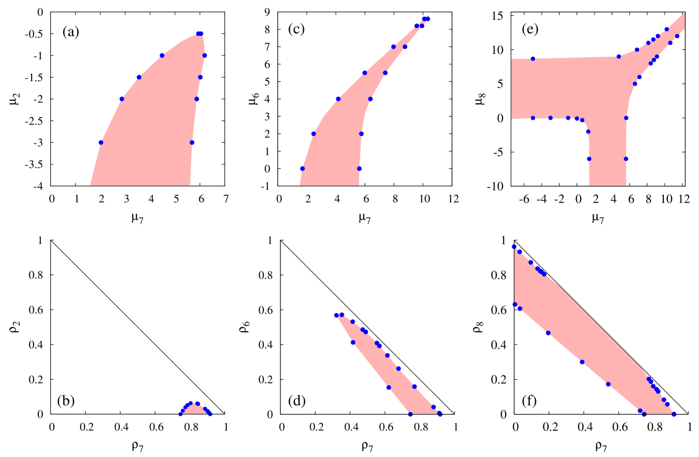
Figure 2: Phase diagram in the $\mu$-plane for mixtures of (a) $2$ and $7$, (c) $6$ and $7$, and (e) $7$ and $8$, and in the $\rho$-plane for (b) $2$ and $7$, (d) $6$ and $7$, and (f) $7$ and $8$. The data points (solid circles) are obtained from Monte Carlo simulations. The shaded regions are guides to the eye and correspond to regions with nonzero nematic order.

A system of monodispersed dimers ($k=2$) does not show any phase transition. Thus, when $\rho_{2}\gg\rho_{7}$ (for 2-7 mixture), we do not expect any phase transition. When $\mu_{2}$ or $\rho_{2}$ is small enough, we observe two transitions as $\mu_{7}$ or $\rho_{7}$ is increased: first from a low-density I phase to an intermediate density N phase and second from the N phase to a high-density I phase [see Fig 2(a) and (b)], as seen for the system of monodispersed rods of length $\geq 7$. The difference between the two critical densities decreases as $\rho_{2}$ is increased and beyond a critical $\rho_{2}$, no transitions are observed. On the other hand, when $\rho_{7}$ is kept fixed and $\rho_{2}$ is increased, utmost one transition is present. One may go from the low-density I phase to the high-density I phase continuously without crossing any phase boundary, suggesting that the high-density I phase is a re-entrant low-density I phase [32].

The phase diagram for 6-7 mixture [see Fig. 2(c) and (d)] is quite similar to that of the 2-7 mixture. The area of the nematic region is larger for the 6-7 mixture, showing that longer rods favor orientational ordering. Unlike the 2-7 mixture, now there are regions where the system undergoes two transitions when $\rho_{7}$ is kept fixed and $\rho_{6}$ is varied. The fully packed line remains disordered for all compositions of 2-7 and 6-7 mixtures. We expect a qualitatively similar phase diagram for mixtures with $k_{1}<7$ and $k_{2}=7$.

Now, consider the 7-8 mixture. This case is different from the above two, as there are two critical points on each of the two axes $\rho_{7}=0$ and $\rho_{8}=0$ [see Fig. 2(e) and (f)]. For small values of $\rho_{7}$ or $\rho_{8}$, two transitions are observed, The high-density I phase is separated from the low-density I phase by a region of N phase. It raises the question whether the system is disordered at full packing as seen for 2-7 and 6-7 mixtures. The algorithm that we use does not equilibrate the system at full packing. Instead, by simulating the system close to full packing, we find that the phase boundaries, separating the N phase from the high-density I phase approach the $\rho=1$ line, and appear to terminate at two separate points [see Fig. 2(f)], suggesting that there are two transitions along the $\rho=1$ line.

All the transitions that we observe are continuous as we do not observe any jump in the density or in the nematic order parameter near the transitions. Also, the nematic order of both the species increases from zero simultaneously with density, and thus we do not observe any fractionation effect.

3.2 Virial Expansion

We now determine the phase diagram of the system from a standard low-density virial expansion for multiple species truncated at the second virial coefficient [19].

Let $N_{k_{i}}^{j}$, where $i=1,2$ and $j=h$ (horizontal), $v$ (vertical), denote the number of rods of length $k_{i}$ with orientation $j$. The partition function of a system of $N$ rods in a volume $V$ is then given by

$$Q_{N}=\frac{V^{N}}{N!4^{N}}\sum_{\{N_{k_{i}^{j}}\}}^{\prime}\frac{N!}{\prod_{i,j}N_{k_{i}}^{j}!}\exp[-\phi(\{N_{k_{i}}^{j}\})],$$ (1)

where the prime denotes the constraint $\sum_{i,j}N_{k_{i}}^{j}=N$, and $\phi_{N}$ is the reduced excess free energy for a given distribution of lengths and orientations:

$$\exp[-\phi_{N}(\{N_{k_{i}}^{j}\})]=\frac{1}{V^{N}}\sum_{\textbf{R}}\exp(-\beta U_{N}),$$ (2)

where $U_{N}$ is the total interaction energy, and R denotes all possible positions.

Let $x_{i}^{j}=N_{k_{i}}^{j}/N$ denote the fraction of rods of length $k_{i}$ with orientation $j$. For large $N$, $V$, (1) may be written as

$$Q_{N}=\int_{0}^{1}\prod_{i,j}dx_{i}^{j}e^{-NF(\{x_{i}^{j}\})}\delta\left(\sum_{i,j}x_{i}^{j}-1\right),$$ (3)

where $F$ is the free energy per particle:

$$F(\{x_{i}^{j}\})=\ln\frac{4\theta}{e}+\sum_{i,j}x_{i}^{j}\ln x_{i}^{j}+\frac{1}{N}\phi_{N}(\{x_{i}^{j}\}),$$ (4)

and $\theta$ is the total number density of rods. For large $N$, the integrals in (3) may be replaced by the largest value of the integrand with negligible error. Thus, the values of $x_{i}^{j}$ are determined by minimizing the free energy in (4).

We compute the reduced excess free energy $\phi_{N}$ as a virial expansion. For a composition $\textbf{x}=(x_{1}^{h},x_{1}^{v},x_{2}^{h},x_{2}^{v})$, the expansion is

$$-\frac{1}{N}\phi_{N}(\theta,\textbf{x})=\sum_{n=2}B_{n}(\textbf{x})\theta^{n-1},$$ (5)

where $B_{n}$ is the $n$-th virial coefficient:

$$B_{n}(\textbf{x})=\frac{1}{Vn!}\sum^{\prime}_{\{n_{k_{i}}^{j}\}}\frac{n!}{\prod_{ij}n_{k_{i}}^{j}}\prod_{ij}(x_{i}^{j})^{n_{k_{i}}^{j}}B(\{n_{k_{i}}^{j}\}).$$ (6)

Here, $n_{k_{i}}^{j}$ is the number of rods of length $k_{i}$ and orientation $j$ in a irreducible graph of size $n$, the prime denotes the constraint $\sum_{i,j}n_{k_{i}}^{j}=n$, and $B(\{n_{k_{i}}^{j}\})=\int\sum\prod f$ is the standard abbreviation for the cluster integrals having Mayer functions $f$ over the irreducible graphs consisting of $n_{k_{i}}^{j}$ rods of length $k_{i}$ and orientation $j$.

We truncate the expansion in (5) at the second virial coefficient. On a lattice, the evaluation of the virial coefficients reduces to the problem of counting the number of disallowed configurations. We thus obtain $B(2,0,0,0)=B(0,2,0,0)=-V(2k_{1}-1)$, $B(0,0,2,0)=B(0,0,0,2)=-V(2k_{2}-1)$, $B(1,0,0,1)=B(0,1,1,0)=-Vk_{1}k_{2}$, $B(1,0,1,0)=B(0,1,0,1)=-V(k_{1}+k_{2}-1)$, $B(1,1,0,0)=-Vk_{1}^{2}$, $B(0,0,1,1)=-Vk_{2}^{2}$. On substituting the virial coefficients into (6), (4) reduces to

$$F(\textbf{x}) = \ln\frac{4\theta}{e}+\sum_{ij}x_{i}^{j}\ln x_{i}^{j}+\frac{\theta}{2}\sum_{ij}(x_{i}^{j})^{2}(2k_{i}-1)$$ (7)

$$+ \theta\sum_{i}k_{i}^{2}\prod_{j}x_{i}^{j}+\theta(k_{1}+k_{2}-1)\sum_{j}\prod_{i}x_{i}^{j}$$

$$+ \theta(x_{1}^{h}x_{2}^{v}+x_{2}^{h}x_{1}^{v})k_{1}k_{2}+O(\theta^{2}).$$

For given densities of the two species, the free energy $F$ in (7) may be expressed in terms of the nematic order parameters of the two species denoted by $\psi_{k_{1}}=(x_{1}^{h}-x_{1}^{v})/(x_{1}^{h}+x_{1}^{v})$ and $\psi_{k_{2}}=(x_{2}^{h}-x_{2}^{v})/(x_{2}^{h}+x_{2}^{v})$. The phase for a given number density is obtained by minimizing $F$ with respect to $\psi_{k_{1}}$ and $\psi_{k_{2}}$. We find existence of only the low-density isotropic-nematic (I-N) transition, similar to the solution of the monodispersed system on a Bethe-like lattice [34]. The I-N phase boundary may be obtained by solving the equation $\frac{\partial^{2}F}{\partial^{2}\psi_{k_{1}}}\frac{\partial^{2}F}{\partial^{2}\psi_{k_{2}}}-\left(\frac{\partial^{2}F}{\partial\psi_{k_{1}}\partial\psi_{k_{2}}}\right)^{2}=0$, and we obtain

$$\frac{(k_{1}-1)^{2}}{k_{1}}\rho_{k_{1}}^{c}+\frac{(k_{2}-1)^{2}}{k_{2}}\rho_{k_{2}}^{c}=2.$$ (8)

By setting $\rho_{k_{2}}^{c}=0$, we obtain the critical density $\rho_{k_{1}}^{c}=2k_{1}/(k_{1}-1)^{2}$, as found earlier for the monodispersed system [52]. For the monodispersed system, the I-N transition exists for lengths larger than $3$.

The phase diagrams for two different mixtures (2-6 and 4-6), obtained from virial expansion are shown in Fig. 3. The shaded (empty) regions correspond to N (I) phases. While the theory predicts the existence of an I-N transition at full packing ($\rho=1$) for 2-4 mixture as the ratio of the densities of the two species are varied [see Fig. 3(a)], for the 4-6 mixture, the fully packed line is always nematic [see Fig. 3(b)]. Within the virial theory, we do not observe any fractionation effect or equivalently, the nematic order for both the rods increases from zero simultaneously as the total density is varied.

The phase diagram obtained from virial expansion differ from those obtained by simulations. It was shown in Ref. [52] that in two dimensions, the higher order virial coefficients do contribute and can not be neglected even in the limit $k_{i}\to\infty$. Thus, truncating the expansion of the reduced excess free energy at the second virial coefficient is only a reasonable approximation at very low densities.

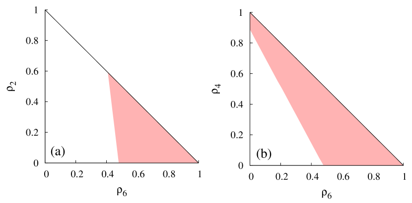
Figure 3: Phase diagram in the $\rho$-plane for mixtures of (a) $2$ and $6$, and (b) $4$ and $6$, obtained from virial expansion. The shaded regions correspond to N phase and the empty regions correspond to I phase.

3.3 Expansion about the pure state along the fully packed line

The fully packed line can neither be numerically studied with the algorithm used in this paper nor with the low-density virial expansion. Instead, we calculate the entropies of the I and N phases as a perturbation expansion about the fully packed monodispersed state. For simplicity, let $k_{1}$ and $k_{2}$ be mutually prime. We approximate the N phase as one where all the rods point in one direction. The arrangement of these rods is a simple combinatorial problem and the entropy per unit site $s_{nem}$, in terms of the number densities of the two species $\theta_{k_{1}}$ and $\theta_{k_{2}}$, is

$$s_{nem}\approx(\theta_{k_{1}}+\theta_{k_{2}})\ln(\theta_{k_{1}}+\theta_{k_{2}})-\theta_{k_{1}}\ln\theta_{k_{1}}-\theta_{k_{2}}\ln\theta_{k_{2}},$$ (9)

where $k_{1}\theta_{k_{1}}+k_{2}\theta_{k_{2}}=1$. Expanding (9) for small $\theta_{k_{2}}$, we obtain

$$s_{nem}\approx-\theta_{k_{2}}\ln\theta_{k_{2}}+O(\theta_{k_{2}}),~{}\theta_{k_{2}}\to 0.$$ (10)

To estimate the entropy of the I phase, we break the lattice into $L/k_{1}$ horizontal strips of width $k_{1}$. The partition function ${\mathcal{L}}_{0}$, when only rods of length $k_{1}$ are present is then,

$${\mathcal{L}}_{0}=2k_{1}\omega_{p}(L)^{L/k_{1}},$$ (11)

where $\omega_{p}(L)$ [$\omega_{o}(L)$] is the partition function for a strip of length $L$ with periodic [open] boundary conditions, and the factor $2k_{1}$ accounts for the two orientations and translational invariance. Clearly, $\omega_{o}(L)=\omega_{o}(L-1)+\omega_{o}(L-k_{1})$ with solution $\omega_{o}(L)=a_{o}\lambda^{L}$, where $\lambda^{k_{1}}-\lambda^{k_{1}-1}-1=0$. Likewise, $\omega_{p}(L)=a_{p}\lambda^{L}$.

Consider defects consisting of rods of length $k_{2}$. To make the system fully packed, a minimum of $k_{1}$ such rods are required. If $k_{1}$ and $k_{2}$ were not mutually prime, this number would change. The smallest contribution to the partition function is when these rods are arranged in a plaquette of size $k_{1}\times k_{2}$ as in Fig. 4(a) or in a vertical line as in Fig. 4(b). Denoting the contribution from these defects as ${\mathcal{L}}_{1}$, we obtain

$${\mathcal{L}}_{1}=2L^{2}z_{k_{2}}^{k_{1}}\omega_{p}(L)^{L/k_{1}}\left[\frac{\omega_{o}(L-k_{2})}{\omega_{p}(L)}+\frac{\omega_{o}(L-1)^{k_{2}}}{\omega_{p}(L)^{k_{2}}}\right].$$ (12)

Figure 4: Defects, made up of rods of length $k_{2}$, that contribute at the lowest order in the perturbation expansion about the fully packed case with only rods of length $k_{1}$.

Substituting for $\omega_{p}$ and $\omega_{o}$ in terms of $\lambda$, we obtain the partition function ${\mathcal{L}}$ to be

$${\mathcal{L}} = 2k_{1}\left[a_{p}\lambda^{L}\right]^{L/k_{1}}\times$$ (13)

$$\left[1+\frac{L^{2}z_{k_{2}}^{k_{1}}}{k_{1}\lambda^{k_{2}}}\left[\frac{a}{a_{p}}+\left(\frac{a}{a_{p}}\right)^{k_{2}}\right]+O\left(z_{k_{2}}^{2k_{1}}.\right)\right]$$

The free energy, $-\ln{\mathcal{L}}$, is in terms of the fugacity. Performing a Legendre transform to obtain entropy in terms of density, we find

$$s_{iso}\approx\frac{\ln\lambda+n_{k_{2}}}{k_{1}}-\frac{n_{k_{2}}}{k_{1}}\ln\left[\frac{n_{k_{2}}\lambda^{k_{2}}}{\frac{a}{a_{p}}+\left(\frac{a}{a_{p}}\right)^{k_{2}}}\right]+\ldots.$$ (14)

For large $k_{1}$, the calculation based on strips gives a good estimation of the entropy. In this limit, $\ln\lambda\approx k_{1}^{-1}\ln k_{1}$ [29]. Equating the entropies for N and I phases [see (10) and (14)], we obtain that along the fully packed line, the system undergoes a isotropic-nematic transition at $\theta_{k_{2}}^{c}\sim k_{1}^{-2}$. Given that the fully packed phase of monodispersed system is isotropic, we expect that there are at least two I-N transitions along the fully packed line, when $k_{1}$ is very large.

4 Discussions

In this letter, we determined the phase diagram of a system of bidispersed hard rods on a square lattice using Monte Carlo simulations, virial expansion and high-density perturbation expansion. Numerically, the phase diagrams of three different mixtures (2–7, 6–7 and 7–8) were determined. For any $2\leq k_{1}\leq 6$ and $k_{2}=7$, the system at full packing is always disordered and the phase diagram is expected to be qualitatively similar to that of 6–7 or 2–7 mixture. When $k_{1},k_{2}\geq 7$, we expect the phase behavior to be qualitatively similar to that of 7–8 mixture, and predict the existence of two transitions at full packing. The low-density virial expansion is able to reproduce the low-density I-N transition but does not work well at high densities. When one of the rod lengths is high enough, the high-density perturbation expansion predicts the existence of two I-N phase transitions along the fully packed line. This prediction could not be verified numerically as the algorithm used in the paper is unsuitable for studying the fully packed line.

Monodispersed hard rectangles have a richer phase diagram than rods, with up to three density driven transitions: from isotropic to nematic to columnar to a solid-like phase [50, 51, 52, 54]. A simple mixture of dimers and squares shows a line of critical points with continuously varying exponents [55]. Polydispersed rectangles are thus expected to have a complicated phase diagram and in three dimensions may show features like fractionation, and therefore is a promising area for future study.

- [1] \NameWen X., Meyer R. B. Caspar D. L. D. \REVIEWPhys. Rev. Lett.6319892760.
- [2] \NameGrelet E. \REVIEWPhys. Rev. Lett.1002008168301.
- [3] \NameDogic Z. Fraden S. \REVIEWPhys. Rev. Lett.7819972417.
- [4] \NameDogic Z. Fraden S. \REVIEWLangmuir1620007820.
- [5] \NameKuijk A., Blaaderen A. v. Imhof A. \REVIEWJ. Am. Chem. Soc.13320112346.
- [6] \NameKuijk A., Byelov D. V., Petukhov A. V., Blaaderen A. v. Imhof A.\REVIEWFaraday Discuss.1592012181.
- [7] \NameBuining P. A. Lekkerkerker H. N. W. \REVIEWJ. Phys. Chem.97199311510.
- [8] \Namevan Bruggen M. P. B., van der Kooij F. M. Lekkerkerker H. N. W.\REVIEWJ. Phys. Condens. Matter819969451.
- [9] \NameCzogalla A., Kauert D. J., Seidel R., Schwille P. Petrov E. P.\REVIEWNano Lett.152015649.
- [10] \Namede Gennes P. G. Prost J. \BookThe Physics of Liquid Crystals(Oxford University Press, Oxford) 1995.
- [11] \NameTaylor D. E., Williams E. D., Park R. L., Bartelt N. C. Einstein T. L. \REVIEWPhys. Rev. B3219854653.
- [12] \NameBak P., Kleban P., Unertl W. N., Ochab J., Akinci G., Bartelt N. C. Einstein T. L. \REVIEWPhys. Rev. Lett.5419851539.
- [13] \NameDünweg B., Milchev A. Rikvold P. A. \REVIEWJ. Chem. Phys.9419913958.
- [14] \NamePatrykiejew A., Sokolowski S. Binder K. \REVIEWSurf. Sci. Rep.372000207.
- [15] \NameLiu D.-J. Evans J. W. \REVIEWPhys. Rev. B6220002134.
- [16] \NameOnsager L. \REVIEWAnn. N.Y. Acad. Sci.511949627.
- [17] \NameBolhuis P. Frenkel D. \REVIEWJ. Chem. Phys1061997666.
- [18] \NameFlory P. J. \REVIEWProc. R. Soc.234195673.
- [19] \NameZwanzig R. \REVIEWJ. Chem. Phys.3919631714.
- [20] \NameVroege G. J. Lekkerkerker H. N. W.\REVIEWRep. Prog. Phys.5519921241.
- [21] \NameStraley J. P. \REVIEWPhys. Rev. A41971675.
- [22] \NameFrenkel D. Eppenga R. \REVIEWPhys. Rev. A3119851776.
- [23] \NameKhandkar M. D. Barma M.Phys. Rev. E722005051717.
- [24] \NameVink R. L. C. \REVIEWEuro. Phys. J. B722009225.
- [25] \NameHeilmann O. J. Lieb E. \REVIEWCommun. Math. Phys.251972190.
- [26] \NameGruber C. Kunz H. \REVIEWCommun. Math. Phys.221971133.
- [27] \NameKunz H. \REVIEWPhys. Lett. A321970311.
- [28] \NameHeilmann O. J. Lieb E. H. \REVIEWPhys. Rev. Lett.2419701412.
- [29] \NameGhosh A. Dhar D. \REVIEWEuro. Phys. Lett.78200720003.
- [30] \NameKundu J., Rajesh R., Dhar D. Stilck J. F. \REVIEWPhys. Rev. E872013032103.
- [31] \NameMatoz-Fernandez D. A., Linares D. H. Ramirez-Pastor A. J.\REVIEWEuro. Phys. Lett82200850007.
- [32] \NameKundu J. Rajesh R. \REVIEWPhys. Rev. E882013012134.
- [33] \NameDisertori M. Giuliani A. \REVIEWCommun. Math. Phys.3232013143.
- [34] \NameDhar D., Rajesh R. Stilck J. F. \REVIEWPhys. Rev. E842011011140.
- [35] \NameHenley C. L.\REVIEWJ. Stat. Phys.891997483
- [36] \NameGhosh A., Dhar D. Jacobsen J. L.\REVIEWPhys. Rev. E752007011115.
- [37] \NameVarga S. Szalai I.\REVIEWPhys. Chem. Chem. Phys.220001955
- [38] \NameSperanza A. Sollich. P.\REVIEWJ. Chem. Phys.11820035213.
- [39] \NameSperanza A. Sollich. P.\REVIEWPhys. Rev. E672003061702.
- [40] \NameLekkerkerker H. N. W, Coulon P. Van Der Haegen R. Deblieck R.\REVIEWJ. Chem. Phys.8019843427.
- [41] \NameBirshtein T. M., Kolegov B. I. PRYAMITSYN V. A.\REVIEWPoly. Sci. U.S.S.R301988316.
- [42] \NameVroege G. J. Lekkerkerker H. N. W.\REVIEWJ. Phys. Chem.9719933601.
- [43] \NameBohle A. M., Holyst R. Vilgis T. \REVIEWPhys. Rev. Lett.7619961396.
- [44] \NameFrenkel D. Bates M. A\REVIEWJ. Chem. Phys.10919986193.
- [45] \NameClarke N., Cuesta J. A., Sear R., Sollich P. Speranza A.\REVIEWJ. Chem. Phys.11320005817.
- [46] \NameMartínez-Ratón Y. Cuesta J. A.\REVIEWJ. Chem. Phys.118200010164.
- [47] \NameStilck J. F. Rajesh R.\REVIEWPhys. Rev. E912015012106.
- [48] \NameIoffe D., Velenik Y. Zahradnik M. \REVIEWJ. Stat. Phys.1222006761.
- [49] \NameKundu J., Rajesh R., Dhar D. Stilck J. F. \REVIEWAIP Conf. Proc.14472012113.
- [50] \NameKundu J. Rajesh R. \REVIEWPhys. Rev. E892014052124.
- [51] \NameKundu J. Rajesh R. \REVIEWEuro. Phys. J. B882014133.
- [52] \NameKundu J. Rajesh R. \REVIEWPhys. Rev. E912015012105.
- [53] \NameNath T. Rajesh R. \REVIEWPhys. Rev. E 902014012120.
- [54] \NameNath T., Kundu J. Rajesh R. \REVIEWJ. Stat. Phys.16020151173.
- [55] \NameRamola K., Damle K. Dhar D. \REVIEWPhys. Rev. Lett.1142015190601.