A Hybrid Approach for Speech Enhancement Using MoG Model and Neural Network Phoneme Classifier

Abstract

In this paper we present a single-microphone speech enhancement algorithm. A hybrid approach is proposed merging the generative Mixture of Gaussians (MoG) model and the discriminative neural network (NN). The proposed algorithm is executed in two phases, the training phase, which does not recur, and the test phase. First, the noise-free speech power spectral density (PSD) is modeled as a MoG, representing the phoneme based diversity in the speech signal. An NN is then trained with phoneme labeled database for phoneme classification with mel-frequency cepstral coefficients (MFCC) as the input features. Given the phoneme classification results, an speech presence probability (SPP) is obtained using both the generative and discriminative models. Soft spectral subtraction is then executed while simultaneously, the noise estimation is updated. The discriminative NN maintain the continuity of the speech and the generative phoneme-based MoG preserves the speech spectral structure. Extensive experimental study using real speech and noise signals is provided. We also compare the proposed algorithm with alternative speech enhancement algorithms. We show that we obtain a significant improvement over previous methods in terms of both speech quality measures and speech recognition results.

I Introduction

Enhancing noisy speech received by a single microphone is a widely-explored problem. A plethora of approaches can be found in the literature [1]. Although many current devices are equipped with multiple microphones, there are still many applications for which only a single microphone is available.

One such application involves automatic speech recognition (ASR) systems. It is well-known that such systems are sensitive to mismatch between the train and test environments. Enhancing the noisy speech signal prior to the application of the ASR system, might alleviate the performance degradation caused by the environment. Nonstationary noise environments are usually more challenging, since the speech enhancement algorithm should adapt to the changing statistics of the additive noise.

The celebrated short-time spectral amplitude estimator (STSA) and log spectral amplitude estimator (LSAE) [2, 3] are widely-used model-based algorithms. The optimally modified log spectral amplitude (OMLSA) estimator and in particular the improved minima controlled recursive averaging (IMCRA) noise estimator are specifically tailored to nonstationary noise environments [4, 5]. However, fast changes in noise statistics often yields the musical noise phenomenon.

Recently, NN techniques gained a lot of popularity due to theoretical and algorithmic progress, and the availability of more data and more processing power. Unlike past learning algorithms for NN, it is now possible to infer the parameters of the NN with many layers, and hence the name deep learning. Deep learning methods were mainly applied to speech recognition and lately, for speech enhancement as well. NN and a deep auto-encoder (DAE) were used as a nonlinear filters in [6] and [7], respectively. The networks are trained on stereo (noisy and clean) audio features, to infer the complex mapping from noisy to clean speech. An experimental study with this approach is shown in [8]. The NN reduces the noise level significantly, yet, the enhanced signals still suffer from noticeable speech distortion.

Other methods attempt to train an NN to find a mask, which classifies the time-frequency bins into speech/noise classes. Given the binary mask, the noisy bins are decreased. In [9] for instance, a support vector machine (SVM) is used to estimate the ideal binary mask (IBM) for speech separation from non-speech background interference. An NN is trained to find the input features for the SVM. A simpler approach is to train the NN itself to find the IBM. Different targets for the NN are presented in  [10]. The IBM has shown advantageous in terms of intelligibility [11]. Yet, the binary mask is known to introduce artifacts such as musical noises. For intelligibility tasks, this might not be problematic, though for speech enhancement the IBM is not sufficient. To circumvent this phenomenon, in [12] the NN is trained to find the ideal ratio mask (IRM), which is a soft mask. A comparison between the IBM and the IRM is presented in [13]. The soft mask is better than the binary mask in terms of speech quality. These approaches do not use models nor assumptions for their speech enhancement. However, they are trained with specific noise types, resulting in poor enhancement in an untrained noise environment. To cope with this problem, in [14] the NN was trained with more than 100 different types of noise. Nevertheless, in real-life where the number of noise types are not limited, this approach may not be satisfactory.

Training-based algorithms, such as MixMax [15], were also developed. These algorithms are performed in two phases, the training phase and the test phase. In the training phase the parameters of the model are found, usually with an unsupervised machine learning algorithms, such as the expectation-maximization (EM) algorithm in [15]. In the test phase, the enhancement is carried out using the learned model parameters. One weakness of the algorithm is that the speech parameters are found in an unsupervised manner that ignores the phoneme-based structure of speech. Another drawback of the MixMax algorithm is that the noise parameters are estimated once at the beginning of the utterance and then are kept fixed during the entire utterance. This enhancement approach is not always sufficient for real-life noises.

In this paper, we apply a hybrid algorithm, which integrates the generative model-based approach with the discriminative NN tool. As in [15], we use a two phase algorithm. In the training phase, the clean speech is modeled with a phoneme-based MoG that is built using phoneme labeled database. A NN is then trained to classify clean time-frame features as one of the phonemes from the phoneme-based MoG. Once the training phase is over, the training does not recur. With the NN estimated phonemes, an SPP is calculated in the test phase using the generative model. Soft spectral subtraction is then carried out using the SPP, while, simultaneously, the noise estimation is updated. The continuity of the speech is maintained using the NN that uses context frames in addition to the current frame. In addition, the NN assists the calculation of the SPP. Furthermore, the phoneme-based MoG and the soft SPP preserve the spectral structure of the speech thus alleviating the musical noise phenomenon. This approach utilizes the benefits of both the generative and the discriminative methods to alleviate the drawbacks of the mentioned above algorithms.

The rest of the paper is organized as follows. In Section II, a generative model is presented. Section III presents the proposed enhancement algorithm and describes its implementation in details. A comprehensive experimental results using speech databases in various noise types are presented in Section IV. In Section V the building blocks of the algorithm are analyzed. Finally, some conclusions are drawn and the paper is summarized in Section VI.

II A Generative Noisy Speech Model

In this section, a generative model of the noisy speech signal is presented. We follow the model proposed by Nádas et al. [16] that was utilized in [15].

The following notation is used throughout the paper. Uppercase letters are used for random variables, lower case for a given value and a boldface symbols denotes vectors.

II-A Maximization approximation

Let $x(t)$ and $y(t)\quad 0<t<T$ denote the speech and noise signals, respectively. The observed noisy signal $z(t)$ is given by

$$z(t)=x(t)+y(t).$$ (1)

Applying the short-time Fourier transform (STFT) with frame length set to $L$ samples and overlap between successive frames set to $3L/4$ samples to $z(t)$ yields $Z(n,k)$ with $n$ the frame index and $k=0,1,\ldots,L-1$ the frequency index. The frame index $n$ is henceforth omitted for brevity, whenever applicable.

Let $\mathbf{Z}$ denote the $L/2+1$ dimensional log-spectral vector, defined by

$${Z}_{k}=\log|Z(k)|,\quad k=0,1,\ldots,L/2.$$

Note that the other frequency bins can be obtained by the symmetry of the discrete Fourier transform (DFT). Similarly, we define $\mathbf{X}$ and $\mathbf{Y}$ to be the log-spectral vectors of the speech and noise signals, respectively.

It is assumed that the noise is statistically independent of the speech signal. Furthermore, it is assumed that both the speech and noise are zero-mean stochastic processes. Due to these assumptions the following approximation can be justified:

$$|Z(k)|^{2}\approx|X(k))|^{2}+|Y(k)|^{2}$$

hence

$$Z_{k}\approx\log(e^{X_{k}}+e^{Y_{k}}).$$

Following Nádas et al. [16], the noisy log-spectral can be further approximated:

$$\mathbf{Z}\approx\max(\mathbf{X},\mathbf{Y})$$ (2)

where the maximization is component-wise over the elements of $\mathbf{X}$ and $\mathbf{Y}$. This approximation was found useful for speech recognition [16], speech enhancement [15, 17] and speech separation tasks [18, 19]. In a speech enhancement task, only the noisy signal $\mathbf{Z}$ is observed, and the aim is to estimate the clean speech $\mathbf{X}$.

II-B Clean speech model - Phoneme based MoG

It is well-known that a speech utterance can be described as a time-series of phonemes, i.e. speech is uttered by pronouncing a series of phonemes [20]. In our approach, we give this observation a probabilistic description, namely the log-spectral vector of the clean speech signal, $\mathbf{X}$, is modelled by a MoG distribution, where each mixture component is associated with a specific phoneme. Unlike [15], that uses unsupervised clustering of the speech frames, we use here a supervised clustering, explicitly utilizing the labels of the phonemes of the training speech signals. Based on the MoG model, the probability density function $f(\mathbf{x})$ of the clean speech $\mathbf{X}$, can be written as

$$f(\mathbf{x})=\sum_{i=1}^{m}c_{i}f_{i}(\mathbf{x})=\sum_{i=1}^{m}c_{i}\prod_{k}f_{i,k}(x_{k})$$ (3)

where $m$ is the number of mixture components and

$$f_{i,k}(x_{k})=\frac{1}{\sqrt{2\pi}\sigma_{i,k}}\exp\left\{-\frac{(x_{k}-\mu_{i,k})^{2}}{2\sigma^{2}_{i,k}}\right\}.$$ (4)

Let $I$ be the phoneme indicator random variable (r.v.) associated with the MoG r.v. $\mathbf{X}$, i.e. $p(I=i)=c_{i}$. The term $f_{i}(\mathbf{x})$ is the Gaussian probability density function (p.d.f.) of $\mathbf{X}$ given that $I=i$. The scalar $c_{i}$ is the probability of the $i$-th mixture and $\mu_{i,k}$ and $\sigma_{i,k}$ are the mean and the standard deviation of the $k$-th entry of the $i$-th mixture Gaussian, respectively. Due to the Fourier transform properties, we neglect any residual correlation between the frequency bins. Since for each class $I=i$ the r.v. $\mathbf{X}$ is Gaussian, the frequency bins are also statistically independent. Consequently, the covariance matrix of each mixture component is diagonal. To set the MoG parameters we used the phoneme-labeled TIMIT database [21, 22] as described in Sec. III-D.

II-C Noisy speech model

Let $\mathbf{Y}$ define the log-spectral vector of the noise signal, and let $g(\mathbf{y})$ denote the p.d.f. of $\mathbf{Y}$. As with the log-spectral vector of the speech signal, it is assumed that the components of $\mathbf{Y}$ are statistically independent. For simplicity, $g(\mathbf{y})$ is modeled as a single Gaussian, with diagonal covariance i.e.,

$$g(\mathbf{y})=\prod_{k}g_{k}(y_{k})$$ (5)

where

$$g_{k}({y_{k}})=\frac{1}{\sqrt{2\pi}\sigma_{Y,k}}\exp\left\{-\frac{(y_{k}-\mu_{Y,k})^{2}}{2\sigma^{2}_{Y,k}}\right\}.$$ (6)

Initial estimation and adaptation the noise parameters will be explained in Sec. III-E.

Using the maximum assumption in the log-spectral vector of the noisy speech $\mathbf{Z}=\max(\mathbf{X},\mathbf{Y})$, as explained above, it can be verified [16] that the p.d.f. of $\mathbf{Z}$ is given by the following mixture model:

$$h(\mathbf{z})=\sum_{i=1}^{m}c_{i}h_{i}(\mathbf{z})=\sum_{i=1}^{m}c_{i}\prod_{k}h_{i,k}(z_{k})$$ (7)

where

$$h_{i,k}(z_{k})=f_{i,k}(z_{k})G_{k}(z_{k})+F_{i,k}(z_{k})g_{k}(z_{k})$$ (8)

such that $F_{i,k}(x)$ and $G_{k}(y)$ are the cumulative distribution functions of the Gaussian densities $f_{i,k}(x)$ and $g_{k}(y)$, respectively. The term $h_{i}(\mathbf{z})$ is the p.d.f. of $\mathbf{Z}$ given that $I=i$.

The generative modeling described above was nicknamed MixMax [15, 16], since it is based on the maximum assumption and on the modelling of the clean speech as a (Gaussian) mixture p.d.f. and the noisy speech is modeled as the maximum of the clean speech and the noise signal. Originally, the mixture components were not associated with phonemes, but rather learned in an unsupervised manner.

III The Neural-Network MixMax Algorithm

In this section, we describe the proposed enhancement algorithm. In Sec. III-A we remind the minimum mean square error (MMSE) estimator based on the MixMax model [15, 16]. We then propose in Sec. III-B a new variant of the estimator that utilizes the same model but allows for better noise reduction. In Sec. III-C an NN approach is introduced as a tool for accurate phoneme classification. Issues regarding the training of the NN are discussed in Sec. III-D. Finally, test-phase noise adaption is discussed in Sec. III-E.

III-A The MMSE based approach

An MMSE of the clean speech $\mathbf{x}$ from measurement $\mathbf{z}$ is obtained by the conditional expectation $\hat{\mathbf{x}}=E(\mathbf{X}|\mathbf{Z}=\mathbf{z})$. Note, that since the p.d.f. of both $\mathbf{x}$ and $\mathbf{z}$ is non-Gaussian, this estimator is not expected to be linear. Utilizing the generative model described in the previous section we can obtain a closed-form solution for the MMSE estimator as follows.

$$\hat{\mathbf{x}}=\sum_{i=1}^{m}p(I=i|\mathbf{Z}=\mathbf{z})E(\mathbf{X}|\mathbf{Z}=\mathbf{z},I=i).$$ (9)

The posterior probability $p(I=i|\mathbf{Z}=\mathbf{z})$ can be easily obtained from (7) by applying the Bayes’ rule:

$$p(I=i|\mathbf{Z}=\mathbf{z})=\frac{c_{i}h_{i}(\mathbf{z})}{h(\mathbf{z})}.$$ (10)

Since the Gaussian covariance matrices of both the speech and the noise models are diagonal, we can separately compute

$$\hat{\mathbf{x}}_{i}=E(\mathbf{X}|\mathbf{Z}=\mathbf{z},I=i)$$

for each frequency bin. For the $k$-th frequency bin we obtain:

$$\hat{x}_{i,k} = E(X_{k}|Z_{k}=z_{k},I=i)$$

$$= \rho_{i,k}z_{k}+(1-\rho_{i,k})E(X_{k}|X_{k}<z_{k},I=i)$$

such that

$$\rho_{i,k}=p(Y_{k}<X_{k}|Z_{k}=z_{k},I=i)=\frac{f_{i,k}(z_{k})G_{k}(z_{k})}{h_{i,k}(z_{k})}$$ (12)

and for the second term in (III-A):

$$E(X_{k}|X_{k}<z_{k},I=i)=\mu_{i,k}-\sigma^{2}_{i,k}\frac{f_{i,k}(z_{k})}{F_{i,k}(z_{k})}.$$ (13)

The closed-form expression for the MMSE estimator of the clean speech $\hat{\mathbf{x}}=E(\mathbf{X}|\mathbf{Z}=\mathbf{z})$ [16] is obtained from (9),(III-A),(12),(13). These expressions are the core of the MixMax speech enhancement algorithm proposed by Burshtein and Gannot [15]. In their approach the MoG parameters of the clean speech are inferred from a database of speech utterances utilizing the EM in an unsupervised manner.

III-B Soft mask estimation of the clean speech

Assuming the maximization model in (2) is valid, $\rho_{i,k}$ was obtained in (12). Summing over all the possible mixture components, we obtain:

$$\rho_{k}=\sum_{i=1}^{m}p(I=i|\mathbf{Z}=\mathbf{z})\rho_{i,k}=p(X_{k}>Y_{k}|\mathbf{Z}=\mathbf{z}).$$ (14)

The term $\rho_{k}$ can be interpreted as the probability that given the noisy speech vector $\mathbf{z}$, the $k$-th frequency bin of the current log-spectral vector $\mathbf{z}$ is originated from the clean speech and not from the noise. The probability $\rho_{k}$ can thus be viewed as a training-based SPP detector, namely the probability that the designated time-frequency bin is dominated by speech. Consequently, $(1-\rho_{k})$ can be interpreted as the posterior probability that the $k$-th bin is dominated by noise.

Using $\rho_{k}$ and (9),(III-A) the $k$-th frequency bin of the MMSE estimator $\hat{\mathbf{x}}=E(\mathbf{X}|\mathbf{Z}=\mathbf{z})$ can be recast as follows:

$$\hat{x}_{k}=\rho_{k}z_{k}+(1-\rho_{k})E(X_{k}|X_{k}<z_{k},\mathbf{Z}=\mathbf{z}).$$ (15)

Hence, given the generative model, the enhancement procedure in (15), substitutes the frequency bins identified as noise with the a priori value drawn from the MoG model and using (13).

The structure of voiced speech PSD consists of dominant spectral lines which recur at multiples of the fundamental frequency (known as pitch). The PSD of different speakers pronouncing the same phoneme share similar properties, but are never identical. Hence, the MoG parameters inferred from multiple speakers, is never individualized to the current speaker and therefore cannot represent the specific periodicity. The phoneme-based MoG parameters are only capable of preserving the general structure of an averaged phoneme. This phenomenon might lead to residual noise even when the algorithm identifies the noise correctly.

To circumvent this phenomenon, we propose to substitute the optimal estimator that uses the MoG parameters with a simpler estimate based on the spectral substraction paradigm, namely:

$$E(X_{k}|X_{k}<z_{k},\mathbf{Z}=\mathbf{z})$$

is substituted by:

$$z_{k}-\beta$$

where $\beta$ is a noise reduction level. It is well-known that the basic spectral subtraction method is prone to musical noise [23][24]. In our proposed method, the estimator also incorporates the soft mask deduced from the SPP, thus potentially alleviating the musical noise phenomenon.

Substituting $(z_{k}-\beta)$ in (15) we obtain the following simplified expression for the estimated clean speech:

$$\hat{x}_{k}=\rho_{k}\cdot z_{k}+(1-\rho_{k})\cdot({z_{k}}-\beta)$$ (16)

or, equivalently

$$\hat{x}_{k}=z_{k}-(1-\rho_{k})\cdot\beta$$ (17)

which can be interpreted as SPP-driven (soft) spectral subtraction algorithm.

III-C Neural network for phoneme classification

The gist of our approach is the calculation of the SPP $\rho_{k}$ (14). This calculation necessitates two terms, $\rho_{i,k}$ which is given by (12) and the posterior phoneme probability $p_{i}\triangleq p(I=i|\mathbf{Z}=\mathbf{z})$. Utilizing the generative model defined in Section II, $p_{i}$ is obtained from (7) by applying the Bayes’ rule:

$$p_{i}=\frac{c_{i}h_{i}(\mathbf{z})}{h(\mathbf{z})}.$$ (18)

This approach exhibits some major shortcomings. Estimating the required noise statistics is a cumbersome task, especially in time-varying scenarios. Furthermore, as the calculation in (18) is carried out independently for each frame, continuous and smooth speech output cannot be guaranteed.

In our approach, (unlike [15]) we adopt a supervised learning approach in which each mixture component of the clean speech is associated with a specific phoneme. Hence the computation of the mixture index posterior probability becomes a phoneme classification task (based on the noisy speech). To implement this supervised classification task, we substitute (18) with an NN that is known to be significantly better than MoG models for phoneme classification tasks (see e.g. [25]).

The NN is trained on a phoneme-labeled clean speech. For each log-spectral vector, $\mathbf{z}$, we calculate the corresponding MFCC features (and their respective delta and delta-delta features). To preserve the continuity of the speech signal, 9 MFCC vectors are concatenated (the current feature vector, 4 past vectors and 4 future vectors) to form the feature vector, denoted $\mathbf{v}$, which is a standard feature set for phoneme classification. This feature vector is used as the input to the NN, and the phoneme label as the corresponding target. The phoneme-classification NN is trained on clean signals. However, as part of the speech enhancement procedure, we apply it to noisy signals. To alleviate the mismatch problem between train and test conditions, we use a standard preprocessing stage for robust phoneme classification, namely cepstral mean and variance normalization (CMVN) [26].

The SPP $\rho_{k}$ is calculated using (14), which requires both $\rho_{i,k}$ and $p_{i}$. While $\rho_{i,k}$ is calculated from the generative model using (12), we propose to replace (18) for calculating $p_{i}$ by a better phoneme-classification method.

It is therefore proposed, to infer the posterior phoneme probability by utilizing the discriminative NN, rather than resorting to the generative MoG model:

$$p_{i}^{\textrm{NN}}=p(I=i|\mathbf{v};\textrm{NN}).$$ (19)

Note, that the compound feature vector $\mathbf{v}$ is used instead of the original log-spectrum $\mathbf{z}$. Finally, the SPP $\rho_{k}$ is obtained using (12) and (19):

$$\rho_{k}=\sum_{i=1}^{m}p_{i}^{\textrm{NN}}\rho_{i,k}.$$ (20)

The proposed SPP calculation is based on a hybrid method, utilizing both the generative MoG model and a discriminative approach to infer the posterior probability. For the latter we harness the known capabilities of the NN.

III-D Training the MoG model and the NN classifier

We used the phoneme-labeled clean speech TIMIT database [21, 22] to train the NN phoneme classifier and the MoG phoneme-based generative model. We next describe the training procedure. We used the 462 speaker from the training set of the database excluding all SA sentences, since they consist of identical sentences to all speakers in the database, and hence can bias the results.

In training the phoneme-based MoG we set the number of Gaussians to $m=39$ (see [27]), where each Gaussian corresponds to one phoneme. All frames labeled by the $i$-th phoneme were grouped, and for each frequency bin the mean and variance were computed using (21) and (22), respectively. First, the log-spectrum of the segments of clean speech utterances is calculated. Since the database is labeled each segment is associated with a phoneme $i$. We can then calculate the following first- and second-moment with phone label $i$:

$$\mu_{i,k} =\frac{1}{N_{i}}\sum_{n=1}^{N_{i}}x_{i,k}(n)$$ (21)

$$\sigma_{i,k}^{2} =\frac{1}{N_{i}-1}\sum_{n=1}^{N_{i}}\left(x_{i,k}(n)-\mu_{i,k}\right)^{2}$$

where $x_{i,k}(n)$ is $k$-th bin of the $n$-th log-spectra vector with phoneme label $i$. The term, $N_{i}$ is the total number of vectors associated with phoneme labeled $i$. The mixture coefficients $c_{i}$ are set to be the relative frequency of each phoneme in the training dataset:

$$c_{i}=\frac{N_{i}}{\sum_{n=1}^{m}N_{n}}.$$ (22)

Note that since the data is already labeled, no iterative clustering procedure, such as the EM algorithm, is required.

For training the NN as a discriminative phoneme classifier, we used the MFCC feature vectors $\mathbf{v}$ powered by the delta and delta-delta coefficients. In total, $39$ coefficients per time frame were used. Context frames (4 from the future and 4 from the past) were added to the current frame as proposed in [28]. Hence, each time frame was represented by 351 MFCC features. We used a single hidden layer NN comprising of 500 neurons. (Although adding more hidden layers slightly improves phoneme classification rate, we didn’t gain any significant improvement in the overall enhancement procedure.) The network is constructed of sigmoid units as the transfer function for the hidden layer:

$$h_{i}=\frac{1}{1+\exp(-\mathbf{w}_{1,i}^{{\scriptscriptstyle\top}}\mathbf{v})},\quad i=1,\ldots,500$$

and a softmax output layer to obtain a vector $m$ probabilities associated with the various phonemes:

$$p(I=i|\mathbf{v})=\frac{\exp(\mathbf{w}_{2,i}^{{\scriptscriptstyle\top}}\mathbf{h})}{\sum_{k=1}^{m}\exp(\mathbf{w}_{2,k}^{{\scriptscriptstyle\top}}\mathbf{h})},\quad i=1,\ldots,m$$

where $\mathbf{w}_{1}$ and $\mathbf{w}_{2}$ are the weights matrices, of the hidden layer and the output layer, respectively. Given a sequence of MFCC feature vectors $\mathbf{v}_{1},..,\mathbf{v}_{N}$, where $N$ is the total number of vectors in the training set, with the corresponding phoneme labels, $I_{1},\ldots,I_{N}\in\{1,\ldots,m\}$, the NN is trained to maximize the log-likelihood function:

$$L({\mathbf{w}_{1},\mathbf{w}_{2}})=\sum_{t=1}^{N}\log p(I_{t}|\mathbf{v}_{t};{\mathbf{w}_{1},\mathbf{w}_{2}}).$$ (23)

To train the network we can start with random weights (or use pre-training methods (see [29])) and then, by applying back-propagation algorithm as part of a gradient ascent procedure, the parameter sets of the network, $\mathbf{w}_{1}$ and $\mathbf{w}_{2}$, are found. In our implementation we used MATLAB$\circledR$ R2014b pattern recognition toolbox [30] to train the NN. The default training function, namely the scaled conjugate gradient back-propagation [31] was used. To avoid mismatch between train and test conditions each utterance was normalized, such that the utterance samples mean and the variance are zero and one, respectively.

To verify the accuracy of the classifier, the trained NN was applied to a clean test set (24-speaker core test set drawn from TIMIT database), obtaining $71\%$ correct phoneme classification results, which is a reasonably high score.

During the test phase of the algorithm, the NN is applied to speech signals contaminated by additive noise. We have therefore applied the CMVN procedure before the classifier to circumvent the noisy test condition [26].

III-E Noise parameter initialization and adaptation

To estimate the noise parameters it is assumed that the first part of the utterance (usually 0.25 Sec) the speech is inactive and it consists of noise-only segments. These first segments can therefore be used for initializing the parameters of the noise Gaussian distribution as follows:

$$\mu_{Y,k} =\frac{1}{N_{Y}}\sum_{n=1}^{N_{Y}}y_{k}(n)$$ (24)

$$\sigma_{Y,k}^{2} ={\frac{1}{N_{Y}-1}\sum_{n=1}^{N_{Y}}\left(y_{k}(n)-\mu_{Y,k}\right)^{2}}$$

where $N_{Y}$ is the number of vectors constructed form the noise-only samples. The term $y_{k}(n)$ denotes the $k$-th bin of the $n$-th noise vector.

In [15], the noise parameters remain fixed for the entire utterance, rendering this estimate incapable of processing non-stationary noise scenarios. To alleviate this problem, we will apply an adaptation procedure (see [5] for alternative noise PSD adaptation techniques). Using the SPP derived in (20), the following adaptation scheme for the noise model parameters can be stated:

$$\mu_{Y,k}^{\textrm{new}}= \rho_{k}\cdot\mu_{Y,k}^{\textrm{old}}+$$ (25)

$$(1-\rho_{k})\left(\alpha\cdot{z_{k}}+(1-\alpha)\cdot\mu_{Y,k}^{\textrm{old}}\right)$$

$$\sigma_{Y,k}^{\textrm{new}}= \rho_{k}\cdot\sigma_{Y,k}^{\textrm{old}}+$$

$$(1-\rho_{k})\left(\alpha\cdot\sqrt{({z_{k}}-\mu_{Y,k}^{\textrm{new}})^{2}}+(1-\alpha)\cdot\sigma_{Y,k}^{\textrm{old}}\right)$$

where $\mu_{Y,k}^{\textrm{new}}$ and $\sigma_{Y,k}^{\textrm{new}}$ are the updated parameters and $\mu_{Y,k}^{\textrm{old}}$ and $\sigma_{Y,k}^{\textrm{old}}$ are the parameters before adaption, and $0<\alpha<1$ is a smoothing parameter. Using this scheme, the noise statistics can be adapted during speech utterances, utilizing the frequency bins that are dominated by noise. This scheme is particularly useful in non-stationary noise scenarios. As a consequence, the first few segments, assumed to be dominated by noise, are only used for initializing the noise statistics and their influence is fading out as more data is collected.

The proposed algorithm is summarized in Algorithm 1. We dub the proposed algorithm neural network mixture-maximum (NN-MM) to emphasize its hybrid nature, as a combination of the generative MixMax model and the phoneme-classification NN.

Train phase:

input: Log-spectral vectors $\mathbf{z}_{1},\ldots,\mathbf{z}_{N}$, MFCC vectors $\mathbf{v}_{1},\ldots,\mathbf{v}_{N}$, and their corresponding phoneme labels $i_{1},\ldots,i_{N}$.

MoG training:

Set the phoneme-based MoG parameters using $(\mathbf{z}_{1},i_{1}),\ldots,(\mathbf{z}_{N},i_{N})$ (21) and (22).

NN training:

Train a NN for phoneme classification using $(\mathbf{v}_{1},i_{1}),\ldots,(\mathbf{v}_{N},i_{N})$.

Test phase:

input: Log-spectral vector of the noisy speech $\mathbf{z}$ and a corresponding MFCC vector $\mathbf{v}$.

output: Estimated log-spectral vector of the clean speech $\hat{\mathbf{x}}$.

Compute the phoneme classification probabilities (19):

$$p_{i}^{\textrm{NN}}=p(I=i|\mathbf{v};\textrm{NN}),\quad i=1,\ldots,m$$

for  k=1:L/2  do

       Compute (12):

$$\rho_{i,k}^{\textrm{MM}}=p(Y_{k}<X_{k}|Z_{k}=z_{k},I=i)=\frac{f_{i,k}(z_{k})G_{k}(z_{k})}{h_{i,k}(z_{k})},\hskip 28.45274pti=1,..,m$$

Compute the speech presence probability (20):

$$\rho_{k}^{\textrm{NN-MM}}=\sum_{i=1}^{m}p_{i}^{\textrm{NN}}\rho_{i,k}^{\textrm{MM}}$$

Estimate the clean speech (17):

$$\hat{x}_{k}=z_{k}-(1-\rho_{k})\cdot\beta.$$

Adapt the noise parameters (25):

$$\mu_{Y,k}^{\textrm{new}}= \rho_{k}\cdot\mu_{Y,k}^{\textrm{old}}+(1-\rho_{k})\left(\alpha\cdot{z_{k}}+(1-\alpha)\cdot\mu_{Y,k}^{\textrm{old}}\right)$$

$$\sigma_{Y,k}^{\textrm{new}}= \rho_{k}\cdot\sigma_{Y,k}^{\textrm{old}}+(1-\rho_{k})\left(\alpha\cdot\sqrt{({z_{k}}-\mu_{Y,k}^{\textrm{new}})^{2}}+(1-\alpha)\cdot\sigma_{Y,k}^{\textrm{old}}\right)$$

end for

Algorithm 1 Summary of the proposed neural network mixture-maximum (NN-MM) algorithm.

IV Experimental study

In this section we present a comparative experimental study. We first describe the experiment setup in Sec. IV-A. Objective quality measure results are then presented in Sec. IV-B. In Sec. IV-C ASR results are compared with different approaches. Finally, the algorithm is tested with an untrained database in Sec. IV-D.

IV-A Experimental setup and quality measures

To test the proposed algorithm we have contaminated speech signal with several types of noise from NOISEX-92 database [32], namely Speech-like, Babble, Car, Room, AWGN and Factory. The noise was added to the clean signal drawn from the test set of the TIMIT database (24-speaker core test set), with 5 levels of signal to noise ratio (SNR) at $-5$ dB, $0$ dB, $5$ dB, $10$ dB and $15$ dB in order to represent various real-life scenarios. The algorithm was tested similarly, with the untrained wall street journal (WSJ) database [33]. We compared the proposed NN-MM algorithm to the OMLSA algorithm [4] with IMCRA noise estimator [5], a state-of-the-art algorithm for single channel enhancement. The default parameters of the OMLSA were set according to [34].

In order to evaluate the performance of the NN-MM speech enhancement algorithm, several objective and subjective measures were used, namely the perceptual evaluation of speech quality (PESQ) quality measure, which has a high correlation with subjective score [35], and a composite measure [36], weighting the log likelihood ratio (LLR), the PESQ and the weighted spectral slope (WSS) [37]. The composite measure outputs background distortion (Cbak), speech distortion (Csig) and overall quality (Covl) results.

As an additional measure we have examined the performance improvement of an ASR system. We used the PocketSphinx ASR system [38]. The feature set of the system is composed of 39 MFCC features powered by delta and delta-delta features. The acoustic model consists of a hidden Markov model with 5000 states. Each state is represented by a MoG with 16 mixture components. Finally, the 20,000-word vocabulary language model was trained using WSJ corpus [33]. Finally, we have carried out informal listening tests.

IV-B Objective results - TIMIT test set

We first evaluate the objective results of the proposed NN-MM algorithm and compare it with the results obtained by the OMLSA algorithm. To further examine the upper bound of the proposed method we also replaced the NN classifier with an ideal classifier that always provides the correct phoneme, denoted ideal-NN-MM. The test set was the core set of the TIMIT database.

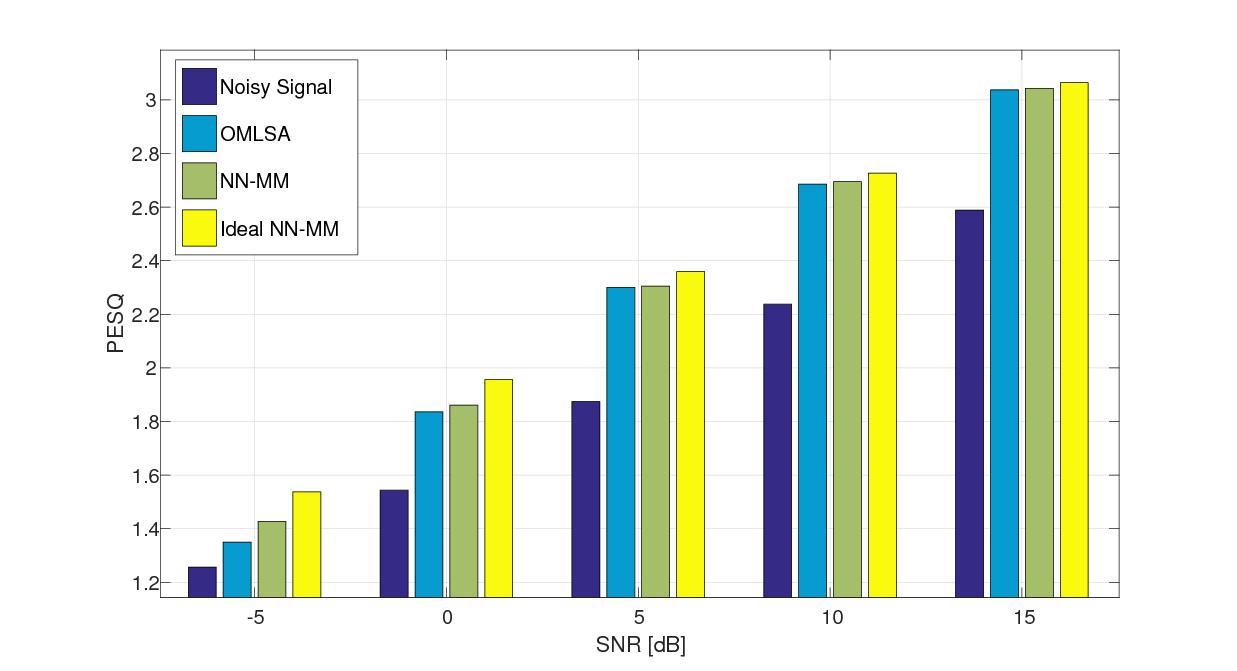
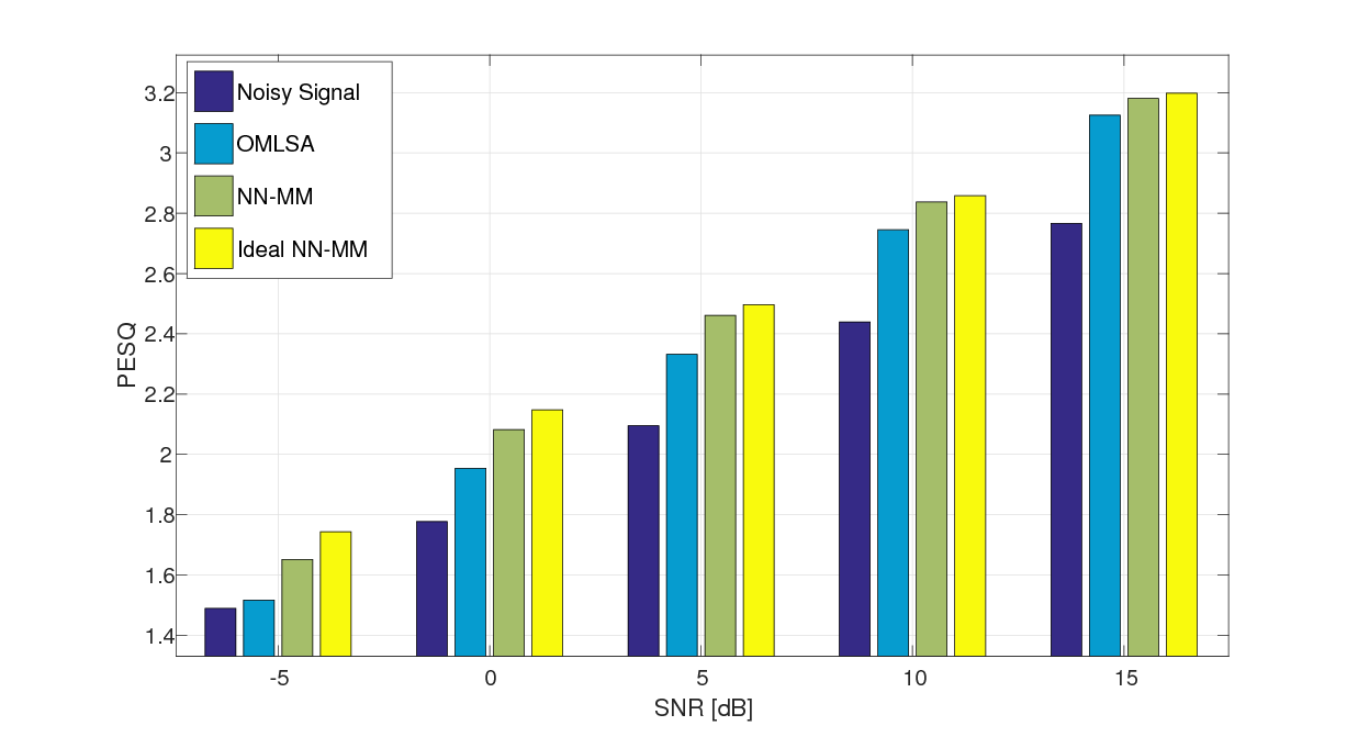
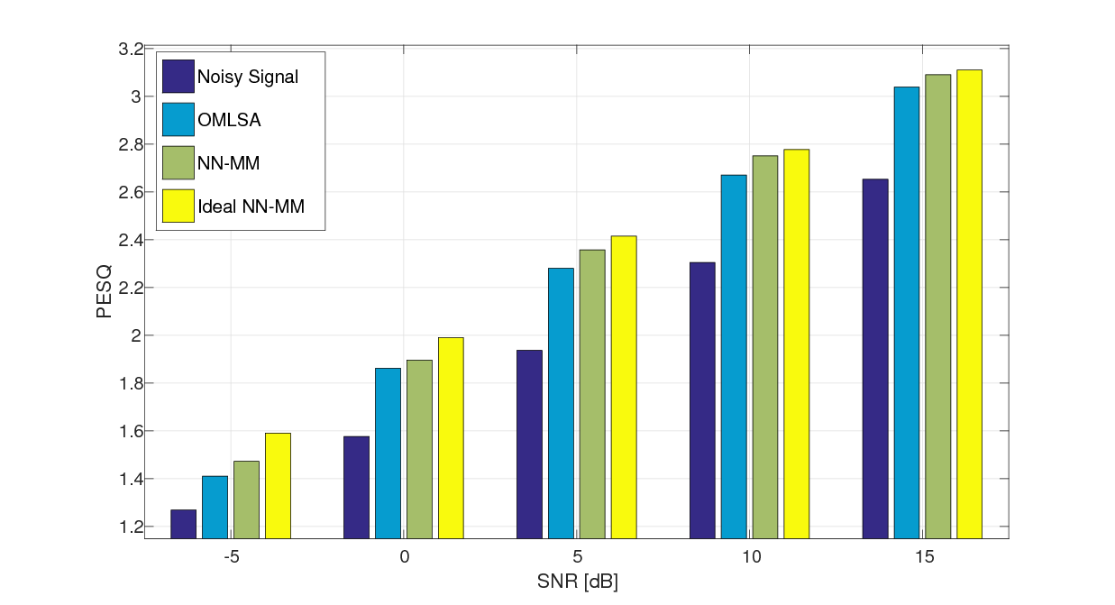
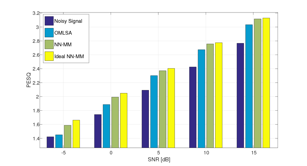
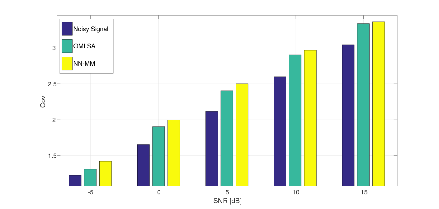
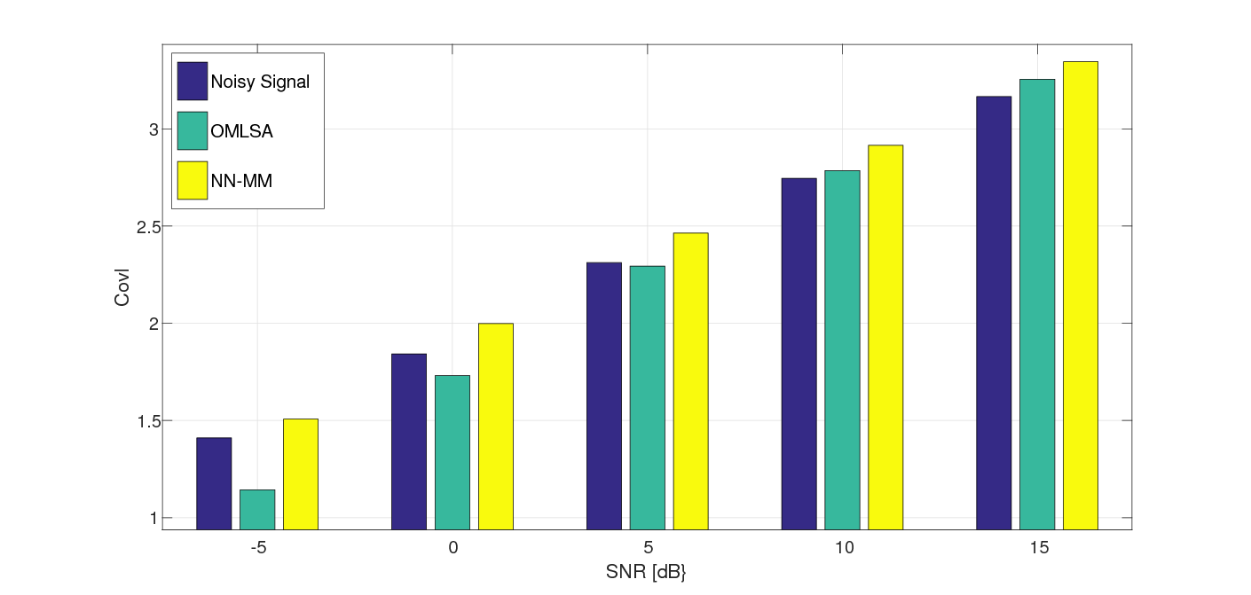
Fig. 1 depicts the PESQ results of all examined algorithm for the Speech-like, Room, Factory and Babble noise types as a function of the input SNR. In Fig. 2 we show the Covl results for factory and room noises. The results behave in a similar way, with other noise types.

It can be clearly deduced that the proposed NN-MM algorithm outperform the OMLSA algorithm in the two designated objective measures. The ideal-NN-MM outperforms the NN-MM, but the difference is rather marginal. Still, there is a room for improvement, would a better phoneme classifier be available.

(a) Speech noise.

(b) Room noise.

(c) Factory noise.

(d) Babble noise.

Figure 1: Speech quality results (PESQ) for several noise types.

(a) Factory noise.

(b) Room noise.

Figure 2: Results of Covl in different noise types.

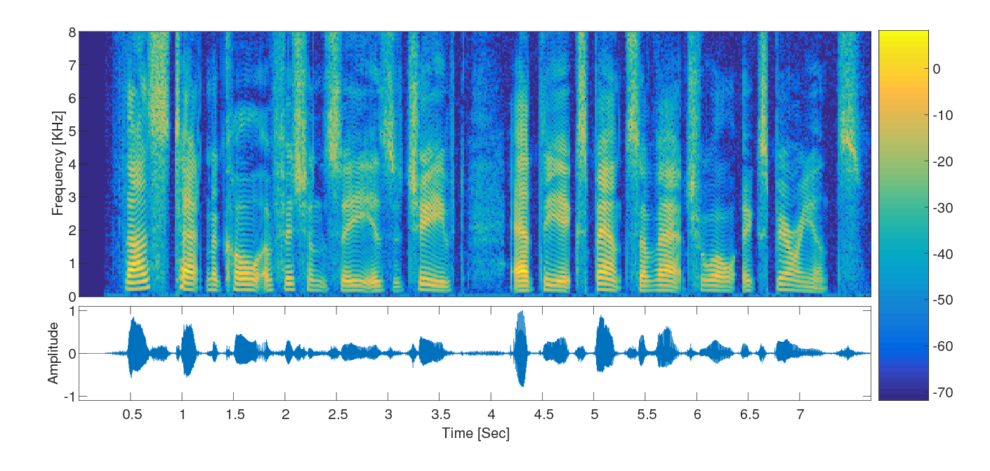
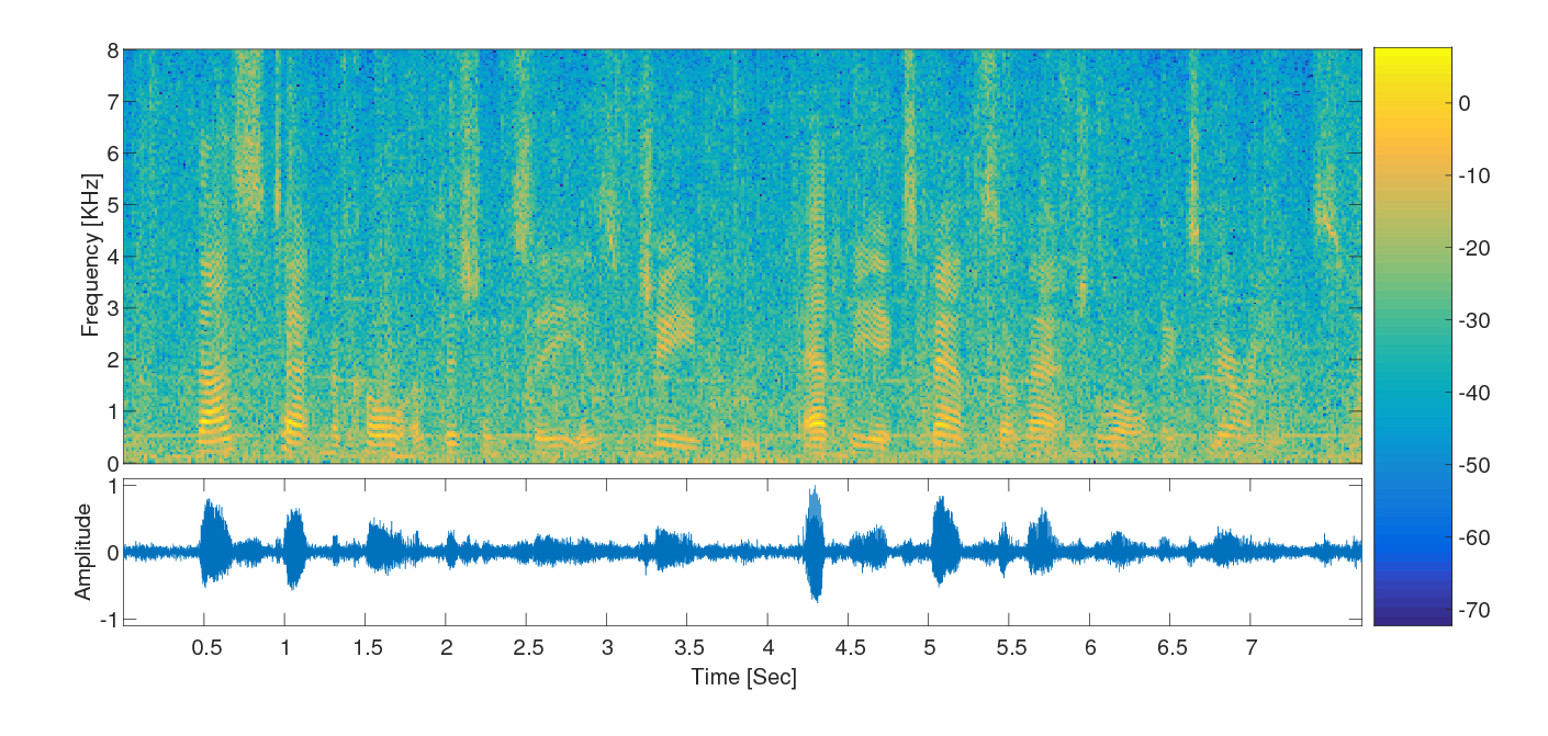
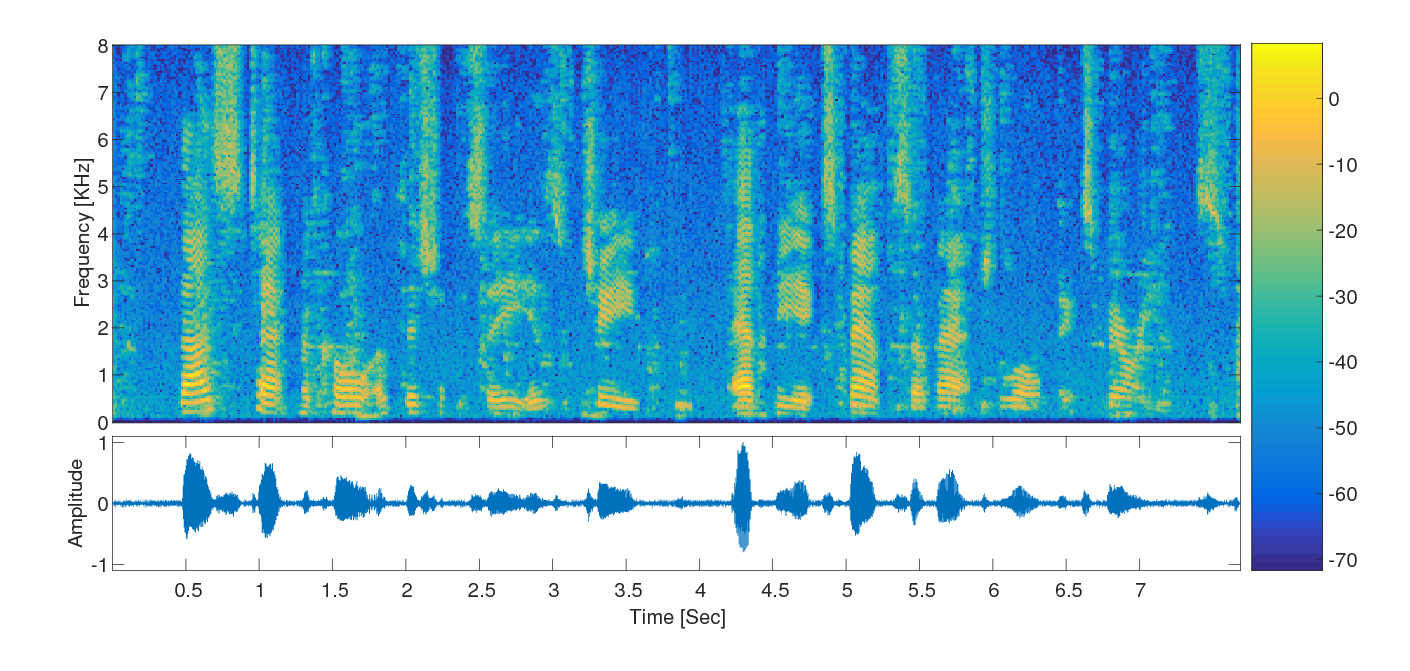
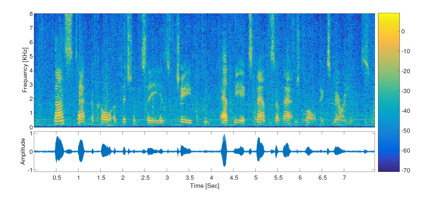
To gain further insight, we have also compared the enhancement capabilities of the proposed algorithm and the state-of-the-art OMLSA algorithm in the challenging factory noise environment. It is clearly depicted in Fig. 3 (obtained in SNR=5 dB) that the proposed NN-MM is less prone to musical noise, while maintaining comparable noise level at the output.

(a) Clean signal.

(b) Noisy signal.

(c) Signal at the output of the OMLSA algorithm.

(d) Signal at the output of the NN-MM algorithm.

Figure 3: STFT and time-domain plots of clean, noisy (factory noise, SNR=5 dB), and signals enhanced by the OMLSA and the NN-MM algorithms.

IV-C Automatic speech recognition results

Speech enhancement algorithms can also serve as a preprocessing stage on front of ASR systems. In order to test the performance of the NN-MM enhancement algorithm we added four types of noise in four different SNR levels to a database comprising five female and five male speakers, each uttering approximately 150 English sentences. The utterances were taken from different speech databases (samples from the WSJ were not included). Overall, the test database consists of 1497 sentences, 2–4 Sec long (2–8 words each).

As before, we have the proposed NN-MM algorithm with the original MixMax and the OMLSA algorithms. The results are depicted in Table I. The NN-MM algorithm significantly outperforms both competing algorithms for the factory and babble noise, and most the speech-like for most SNR values (besides 5 dB). In the white noise case, the original MixMax exhibits slightly better performance. The superior results of the proposed NN-MM algorithm can be attributed to the improved phoneme classification, which is one of the main building blocks of an ASR system.

TABLE I: ASR results for various noise types.

Babble noise
Method \SNR	5[dB]	10[dB]	15[dB]	20[dB]
Noisy signal	8.8	43.0	68.8	79.7
MixMax	18.7	53.7	72.9	81.0
OMLSA	13.7	45.0	66.0	76.2
NN-MM	28.2	60.3	76.2	81.9

Factory noise
Method \SNR	5[dB]	10[dB]	15[dB]	20[dB]
Noisy signal	1.1	32.7	62.2	76.1
MixMax	9.5	44.4	68.3	78.7
OMLSA	16.3	47.4	69.0	78.0
NN-MM	19.5	52.9	71.9	80.1

Speech-like noise
Method \SNR	5[dB]	10[dB]	15[dB]	20[dB]
Noisy signal	7.9	44.4	68.4	77.5
MixMax	38.5	64.9	77.4	81.6
OMLSA	41.3	65.4	75.8	81.3
NN-MM	40.4	66.6	78.0	82.2

White noise
Method \SNR	5[dB]	10[dB]	15[dB]	20[dB]
Noisy signal	10.4	31.8	53.6	68.9
MixMax	28.9	51.7	67.2	77.1
OMLSA	25.8	46.1	65.1	74.5
NN-MM	26.1	45.8	65.5	75.8

IV-D Performance with different database

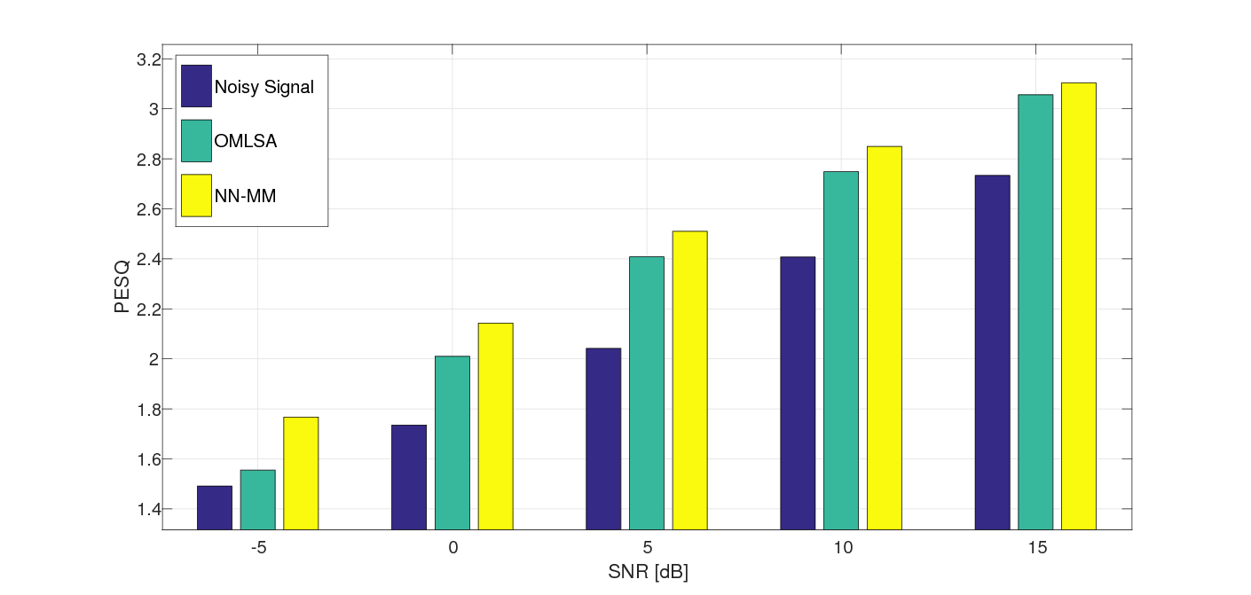
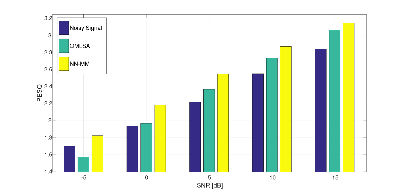
Finally, we would like to demonstrate the capabilities of the proposed NN-MM algorithm when applied to speech signals from other databases. In this work we have trained the phoneme-based MoG and the NN using the TIMIT database. In this section we apply the algorithm to $30$ clean signals drawn from the WSJ database [33]. The signals were contaminated by the challenging factory and babble noise with several SNR levels. Note, that the algorithm does not train with noisy signals. Fig. 4 depicts the PESQ measure of the NN-MM algorithm in comparison with the OMLSA algorithm. It is that the performance of proposed algorithm and its advantages are maintained even for sentences from different database than the training database. Here we show the challenging factory and Babble noise types. The results in other noise types have the same construction.

(a) Factory noise.

(b) Babble noise.

Figure 4: PESQ results with WSJ database for various SNR levels.

V Analysis of the building blocks of the algorithm

In this section, we analyze the individual contributions of each component of the proposed algorithm to the overall performance. First, in Sec. V-A the phoneme-based MoG is analyzed. In Sec. V-B example of the SPP is presented and the NN phoneme classifier is compared to the generative approach in Sec. V-C. Finally, in Sec. V-D the noise adaptation is tested in real-life scenario.

V-A The Phoneme-based MoG

One of the major differences between the original MixMax algorithm and the proposed NN-MM algorithm is the construction of the MoG model. While the former uses unsupervised clustering procedure based on the EM algorithm, the latter uses supervised clustering using the labeled phonemes. Consequently, the clusters in the proposed algorithm consists of different variants of the same phoneme, while the cluster obtained by the EM algorithm mixtures of various phonemes. We postulate that the supervised clustering is therefore advantageous over the unsupervised clustering. We will examine this claim in the current section, using clean speech signal contaminated by Room noise with SNR=5 dB.

First, define the averaged PSD of the speech utterance as the weighted sum of the Gaussian centroids, as inferred by the two clustering procedures. The weights give the respective posterior probabilities (either (10) or (19)). The averaged PSD obtained by the supervised clustering and the discriminative NN is given by:

$$\overline{\mu}_{k}^{\textrm{NN-MM}}=\sum_{i=1}^{m}p_{i}^{\textrm{NN}}\mu_{i,k}.$$ (26)

Similarly, the averaged PSD obtained by the unsupervised clustering and the generative model is given by

$$\overline{\mu}_{k}^{\textrm{EM}}=\sum_{i=1}^{m}p_{i}\mu_{i,k}^{\textrm{EM}}.$$ (27)

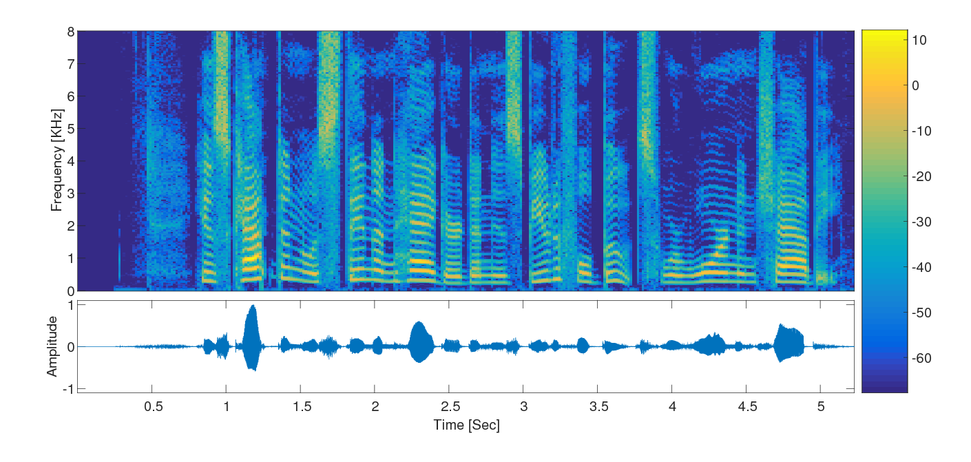
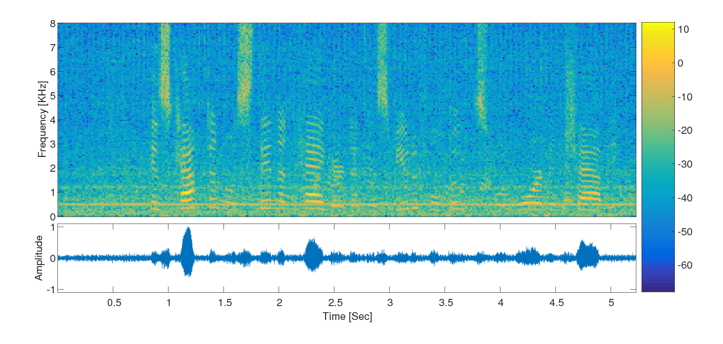
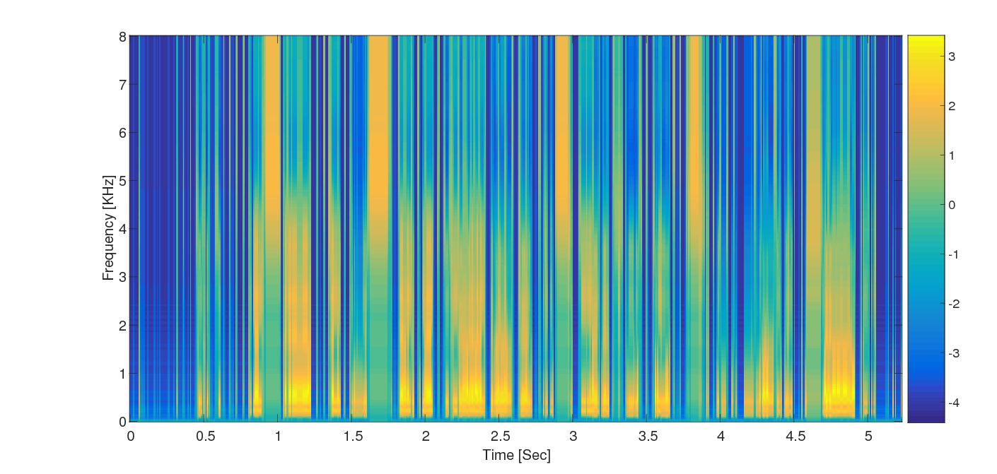
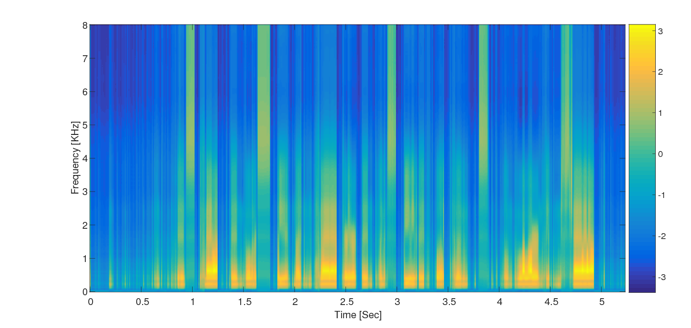
In Figs. 5(a) and 5(b) we show the clean and noisy PSD, respectively. Fig. 5(c) and Fig. 5(d) illustrates the estimated weighted Gaussians $\overline{\mu}^{\textrm{NN-MM}}$ and $\overline{\mu}^{\textrm{EM}}$. It evident that $\overline{\mu}^{\textrm{EM}}$ is not as successful as successful as $\overline{\mu}^{\textrm{NN-MM}}$ in estimating the clean speech PSD.

(a) Clean signal

(b) Noisy signal

(c) $\overline{\mu}^{\textrm{EM}}$ (Log-spectrum).

(d) $\overline{\mu}^{\textrm{NN-MM}}$ (Log-spectrum).

(e) $\rho^{\textrm{EM}}$ parameter.

(f) $\rho^{\textrm{NN-MM}}$ parameter.

(g) MixMax Enhanced.

(h) NN-MM Enhanced.

Figure 5: STFT of the clean, noisy and enhanced signals together with the averaged PSDs and the SPPs using either the NN-MM model or the original MixMax model.

V-B The speech presence probability

The SPP is the probability that the time-frequency bin is dominated by speech. In this section we examine the SPP $\rho_{k}^{\textrm{NN-MM}}$ developed in this work as given in Algorithm 1. To further validate the advantages of the hybrid scheme we compare it with the SPP used in the original MixMax, namely the posterior probabilities are inferred from the generative model and the MoG is trained in an unsupervised manner. The latter SPP is denoted $\rho^{\textrm{EM}}$

We continue the example in Sec. V-A. Both SPPs, $\rho^{\textrm{EM}}$ and $\rho^{\textrm{NN-MM}}$, are depicted in Figs. 5(e) and 5(f), respectively. It can be easily observed that $\rho^{\textrm{NN-MM}}$ has a better resemblance to the clean speech spectrogram shown in Fig. 5(a) and suffers from less artifacts. Additionally, it is smoother than the $\rho^{\textrm{EM}}$ in both time and frequency aspects. Conversely, vertical narrow spectral lines can be easily observed in $\rho^{\textrm{EM}}$. This spectral artifacts may be one of the causes for the differences in the enhancement capabilities of the two algorithms, as depicted in Figs. 5(e) and 5(f).

We postulate that the designated advantages of the proposed approach stem from the better classification capabilities as exhibited by the NN. While the original MixMax algorithm is only utilizing the current frame for inferring the posterior probabilities, the proposed algorithm takes into account the context of the phoneme by augmenting past and future frames to the current frame. This guarantees a smoother SPP and consequently less artifacts at the output of the algorithm.

This context-aware feature vector together with the phoneme-based MoG may also alleviate the musical noise phenomenon. This observation is also supported by the smoother spectral envelop of the MoG centroid as can be deduced from comparing Figs. 5(c) and 5(d).

V-C Phoneme classification task

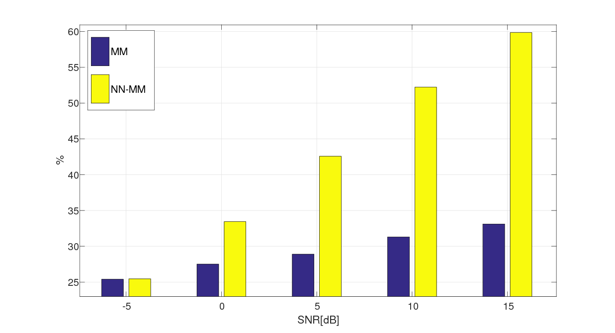
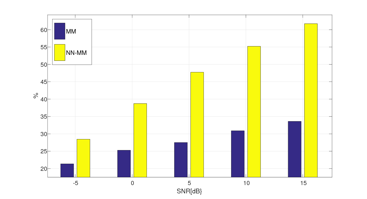
We turn now to the assessment of the proposed phoneme classifier. For that we compare the classification accuracy of the NN with that of the generative model in (10) using the phoneme-labeled MoG.

Fig. 6 depicts the percentage of correct classification results obtained on the test data. Two types of noise were added to the clean signals, namely factory and babble noise. The results clearly indicate that the NN based classifier significantly outperforms the classifier based on the generative model, and hence better suited for the task at hand.

(a) Factory noise.

(b) Babble noise.

Figure 6: Results of phoneme classification task performed on noisy data.

(a) Clean signal.

(b) Noisy signal (SNR=5 dB).

(c) Real noise (Log-spectrum).

(d) Estimated noise (Log-spectrum).

(e) OMLSA enhanced.

(f) NN-MM enhanced.

Figure 7: Noise adaptation capabilities with highly non-stationary siren noise (SNR=5 dB), and the outputs of the OMLSA and NN-MM algorithms.

V-D The Noise adaptation

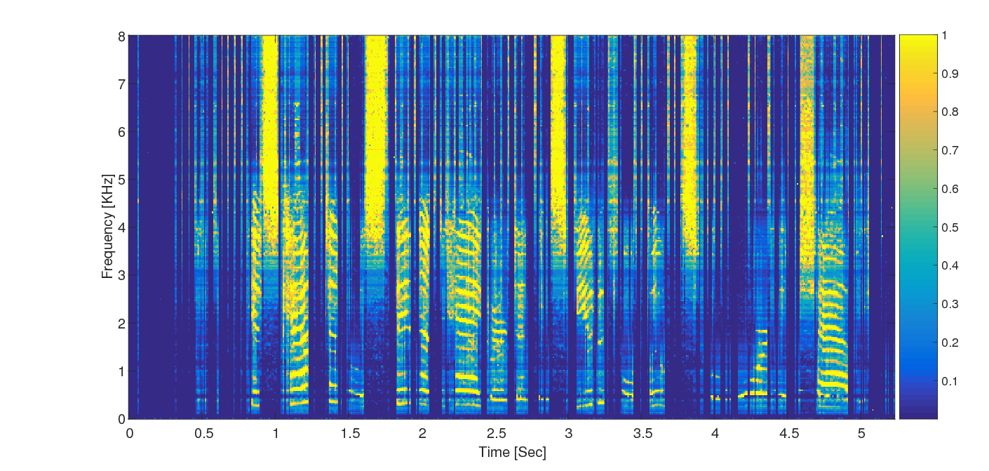
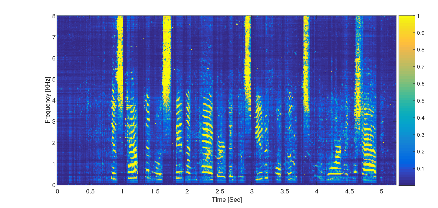
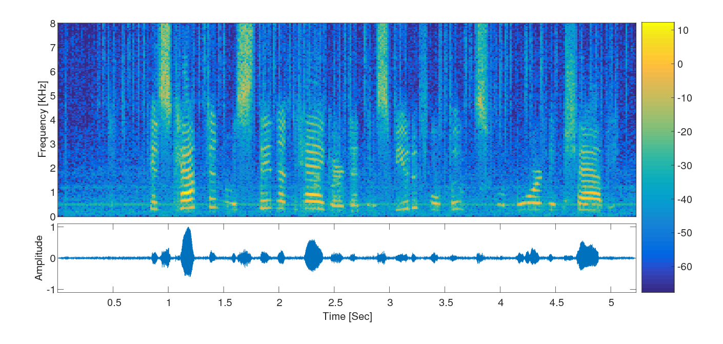
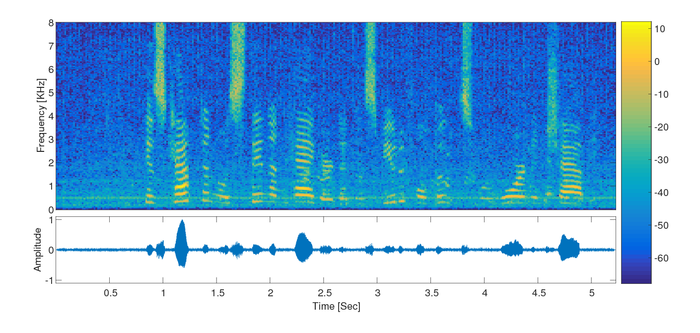
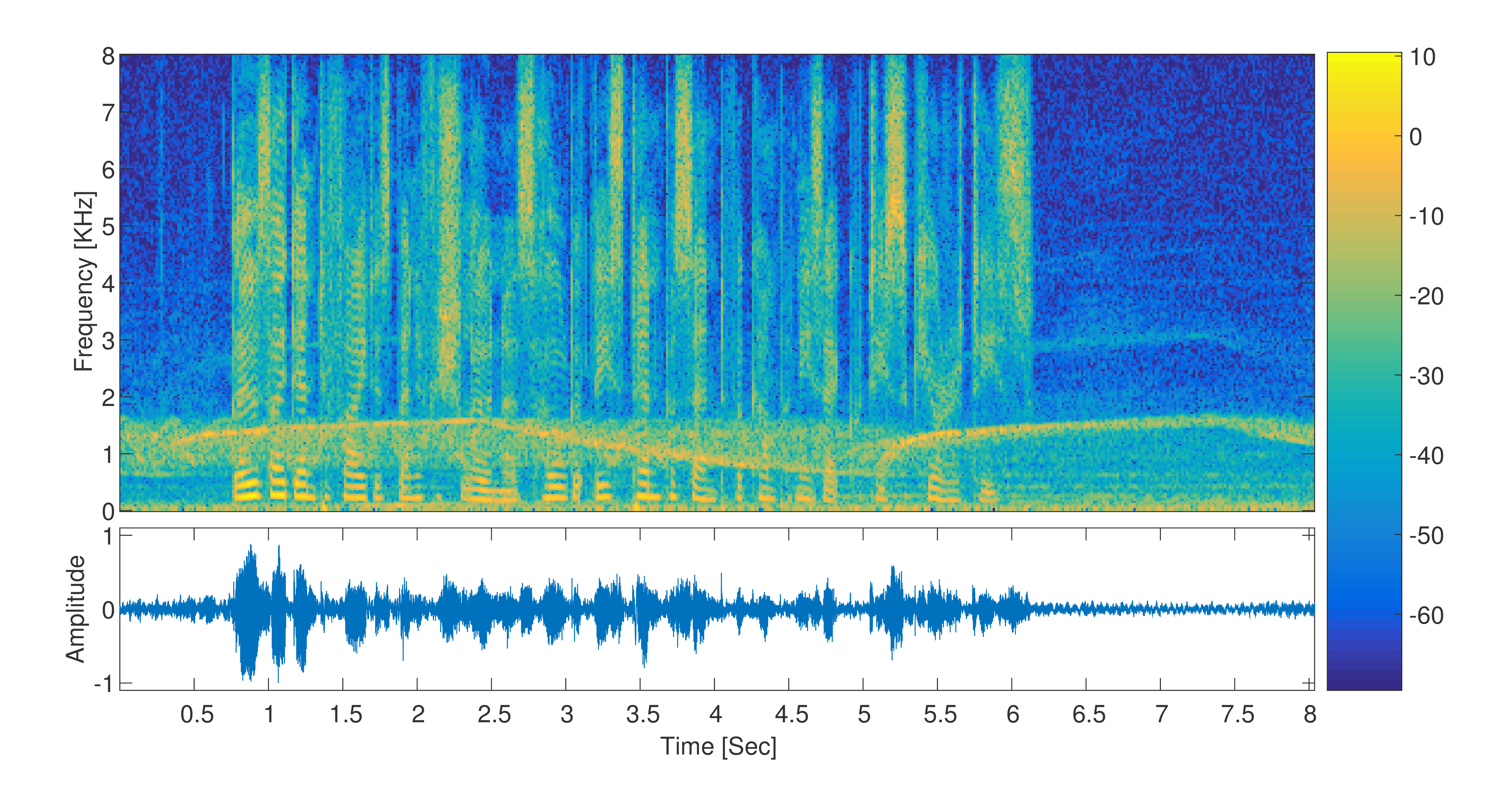
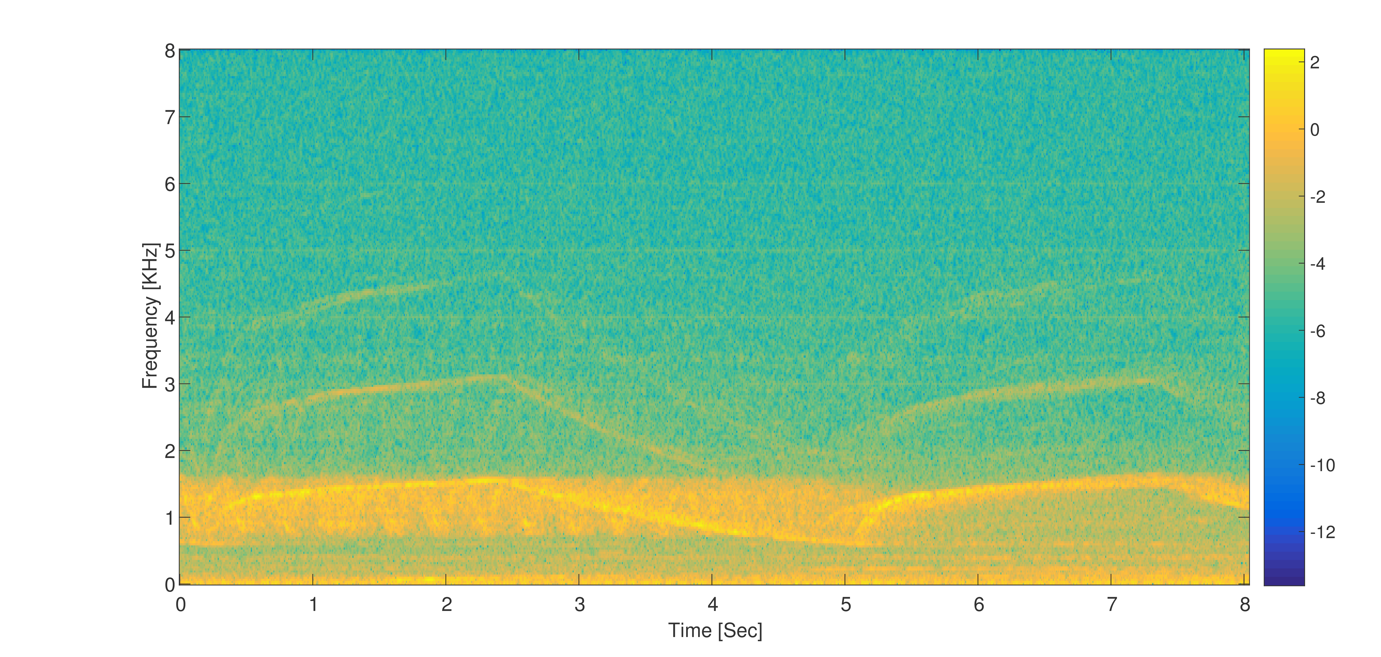
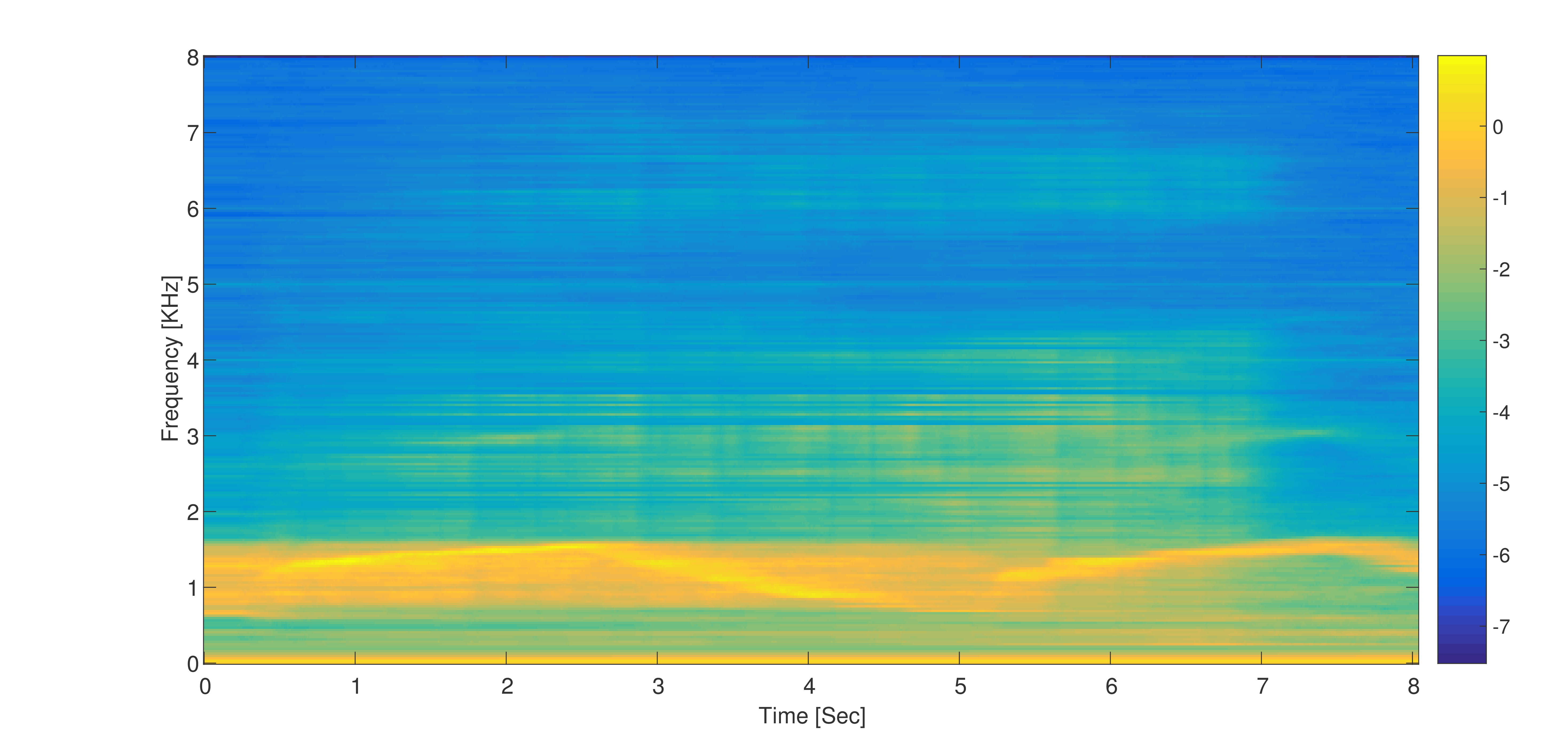
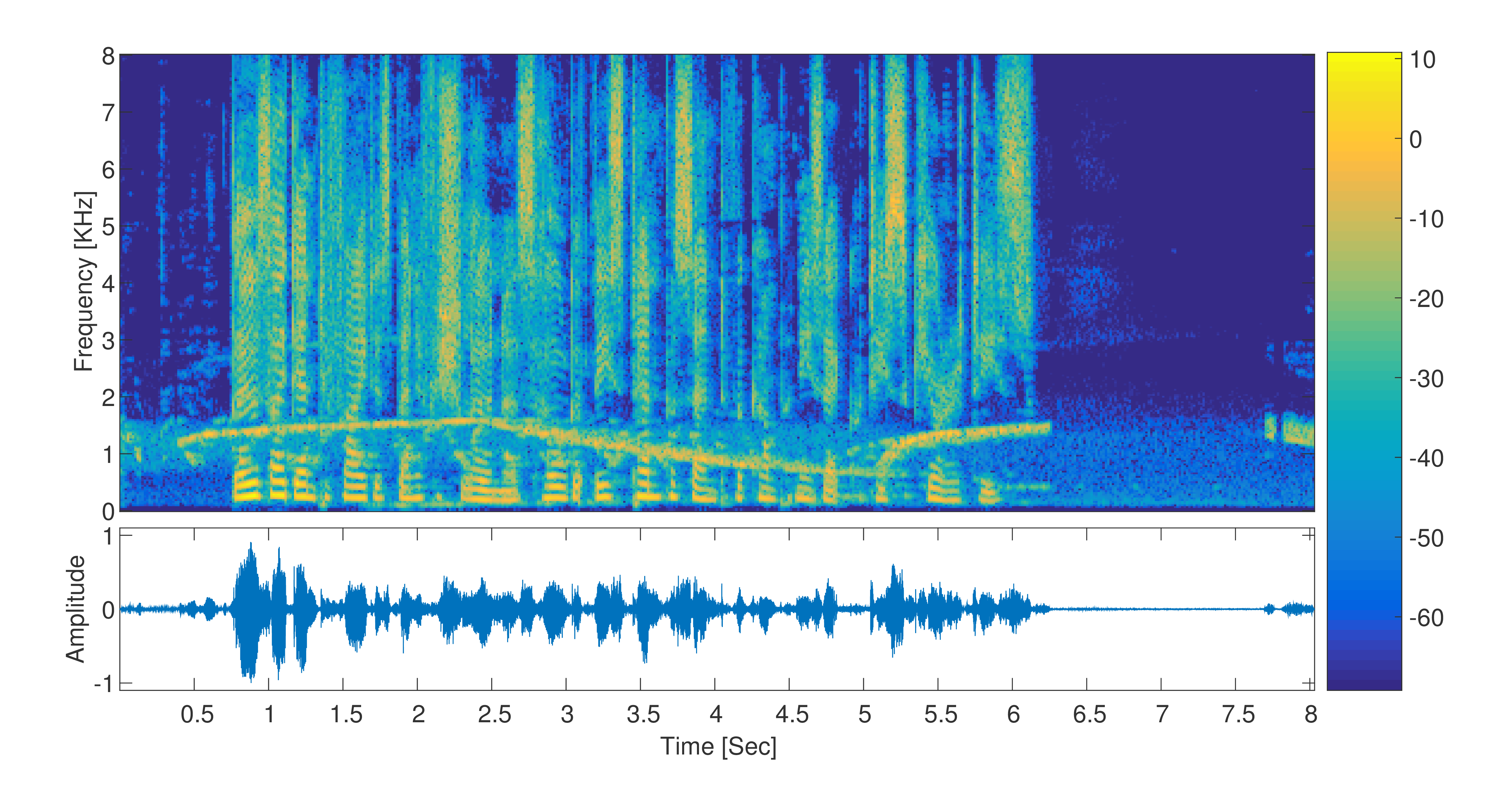
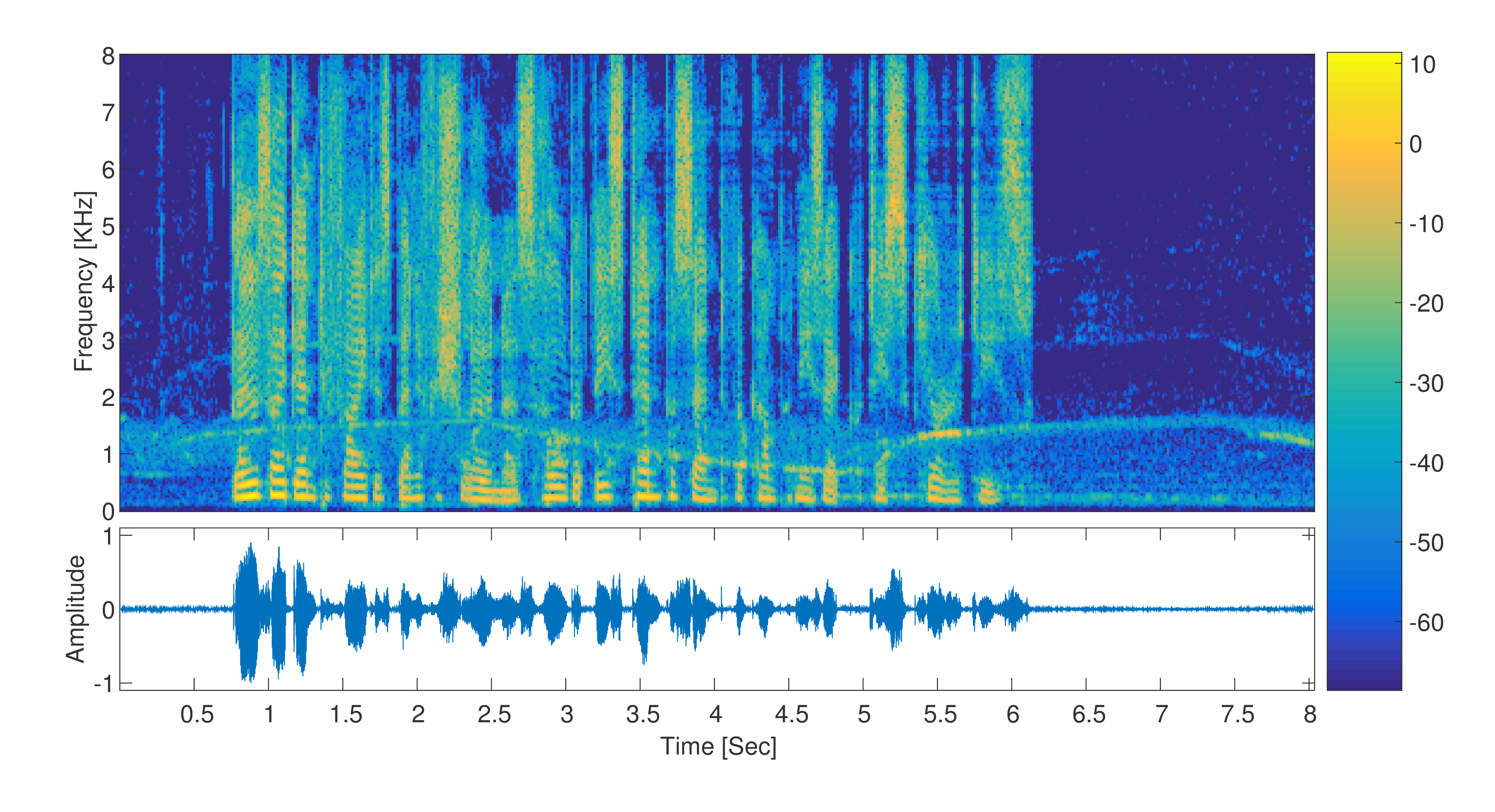
In this section we examine the noise adaptation scheme described in (25). A city ambiance noise [39] that consists of a siren and passing cars was chosen, as it is a highly non-stationary noise source with fast PSD changes during the speech utterance. The clean and noisy signals are depicted in Figs. 7(a) and 7(b). The input SNR was set to 5 dB (resulting in input PESQ=2.124.

In Fig. 7(c) the real noise STFT is depicted and in Fig. 7(d) its estimate using the proposed adaptation scheme and the SPP inferred by the NN-MM algorithm. It can be observed that the estimate is quite accurate even when the noise PSD changes very fast. Note that during speech dominant time-frequency bins, the noise estimate cannot adapt. These adaptation capabilities are also reflected at the output of the algorithms, especially in comparison with the OMLSA algorithm, as depicted in Figs. 7(e) and 7(f). We observe that the NN-MM algorithm outperforms the OMLSA in reducing this challenging noise. This is also indicated by the PESQ measure. While the OMLSA degrade the speech quality (PESQ=1.847), the proposed hybrid algorithm slightly improves it (PESQ=2.361). The reader is also referred to our website where these sound clips can be found.

VI Conclusion

In this paper a novel speech enhancement scheme, denoted NN-MM, is presented. The proposed algorithm is based on a hybrid scheme which combines phoneme-based generative model for the clean speech signal with a discriminative, NN-based SPP estimator. In the proposed algorithm we try to adopt the advantages of model-based approaches and NN approaches. While the former usually trade-off noise reduction abilities with residual musical noise, the latter often suffer from speech distortion artifacts.

In the proposed algorithm we take advantage of the discriminative nature of the NN that preserves speech smoothness by using context frames. Moreover, the phoneme-based MoG model, where each Gaussian corresponds to a specific phoneme, preserves the general phoneme structure and reduces musical noise.

The proposed algorithm requires neither noise samples nor noisy speech utterances to train. Alternatively, using the embedded NN-based SPP, allows for fast adaptation to fast-changing noise PSD.

A comprehensive set of experiments demonstrate the capabilities of the proposed algorithm in both improving ASR scores as well as objective quality measures. The NN-MM algorithm is shown to outperform state-of-the-art algorithm (OMLSA) for both stationary and non-stationary environmental noises and a variety of SNR levels.

References

- [1] P. C. Loizou, Speech enhancement: theory and practice. CRC press, 2013.
- [2] Y. Ephraim and D. Malah, “Speech enhancement using a minimum-mean square error short-time spectral amplitude estimator,” IEEE Trans. on Acoustics, Speech and Signal Processing, vol. 32, no. 6, pp. 1109–1121, Dec 1984.
- [3] ——, “Speech enhancement using a minimum mean-square error log-spectral amplitude estimator,” IEEE Trans. on Acoustics, Speech and Signal Processing, vol. 33, no. 2, pp. 443–445, Apr 1985.
- [4] I. Cohen and B. Berdugo, “Speech enhancement for non-stationary noise environments,” Signal processing, vol. 81, no. 11, pp. 2403–2418, 2001.
- [5] ——, “Noise estimation by minima controlled recursive averaging for robust speech enhancement,” IEEE Signal Processing Letters, vol. 9, no. 1, pp. 12–15, Jan 2002.
- [6] Y. Xu, J. Du, L.-R. Dai, and C.-H. Lee, “An experimental study on speech enhancement based on deep neural networks,” IEEE Signal Processing Letters, vol. 21, no. 1, pp. 65–68, Jan 2014.
- [7] X. Lu, Y. Tsao, S. Matsuda, and C. Hori, “Speech enhancement based on deep denoising autoencoder.” in Proceedings of the annual conference of the International Speech Communication Association (INTERSPEECH), 2013, pp. 436–440.
- [8] D. Liu, P. Smaragdis, and M. Kim, “Experiments on deep learning for speech denoising,” in Proceedings of the annual conference of the International Speech Communication Association (INTERSPEECH), 2014.
- [9] Y. Wang and D. Wang, “Towards scaling up classification-based speech separation,” IEEE Trans. on Audio, Speech, and Language Processing, vol. 21, no. 7, pp. 1381–1390, July 2013.
- [10] Y. Wang, A. Narayanan, and D. Wang, “On training targets for supervised speech separation,” IEEE Trans. on Audio, Speech, and Language Processing, vol. 22, no. 12, pp. 1849–1858, Dec 2014.
- [11] D. Wang, U. Kjems, M. S. Pedersen, J. B. Boldt, and T. Lunner, “Speech intelligibility in background noise with ideal binary time-frequency masking,” The Journal of the Acoustical Society of America, vol. 125, no. 4, pp. 2336–2347, 2009. [Online]. Available: http://scitation.aip.org/content/asa/journal/jasa/125/4/10.1121/1.3083233
- [12] S. Srinivasan, N. Roman, and D. Wang, “Binary and ratio time-frequency masks for robust speech recognition,” Speech Communication, vol. 48, no. 11, pp. 1486–1501, 2006, robustness Issues for Conversational Interaction. [Online]. Available: http://www.sciencedirect.com/science/article/pii/S0167639306001129
- [13] C. Hummersone, T. Stokes, and T. Brookes, “On the ideal ratio mask as the goal of computational auditory scene analysis,” in Blind Source Separation, ser. Signals and Communication Technology, G. R. Naik and W. Wang, Eds. Springer Berlin Heidelberg, 2014, pp. 349–368. [Online]. Available: http://dx.doi.org/10.1007/978-3-642-55016-4_12
- [14] Y. Xu, J. Du, L.-R. Dai, and C.-H. Lee, “A regression approach to speech enhancement based on deep neural networks,” IEEE Trans. on Audio, Speech, and Language Processing, vol. 23, no. 1, pp. 7–19, Jan 2015.
- [15] D. Burshtein and S. Gannot, “Speech enhancement using a mixture-maximum model,” IEEE Trans. on Speech and Audio Processing, vol. 10, no. 6, pp. 341–351, Sep 2002.
- [16] A. Nádas, D. Nahamoo, and M. Picheny, “Speech recognition using noise-adaptive prototypes,” IEEE Trans. on Acoustics, Speech and Signal Processing, vol. 37, no. 10, pp. 1495–1503, Oct 1989.
- [17] Y. Yeminy, S. Gannot, and Y. Keller, “Speech enhancement using a multidimensional mixture-maximum model,” in International Workshop on Acoustic Echo and Noise Control (IWAENC), 2010.
- [18] S. T. Roweis, “One microphone source separation,” in Neural Information Processing Systems (NIPS), vol. 13, 2000, pp. 793–799.
- [19] M. Radfar and R. Dansereau, “Single-channel speech separation using soft mask filtering,” IEEE Trans. on Audio, Speech, and Language Processing, vol. 15, no. 8, pp. 2299–2310, Nov 2007.
- [20] J. H. Hansen, M. Clements et al., “Constrained iterative speech enhancement with application to speech recognition,” IEEE Trans. on Signal processing, vol. 39, no. 4, pp. 795–805, 1991.
- [21] A. Mohamed, G. Dahl, and G. Hinton, “Acoustic modeling using deep belief networks,” IEEE Trans. on Audio, Speech, and Language Processing, vol. 20, no. 1, pp. 14–22, Jan. 2012.
- [22] J. S. Garofolo, L. D. Consortium et al., TIMIT: acoustic-phonetic continuous speech corpus. Linguistic Data Consortium, 1993.
- [23] S. Boll, “Suppression of acoustic noise in speech using spectral subtraction,” IEEE Trans. on Acoustics, Speech and Signal Processing, vol. 27, no. 2, pp. 113–120, Apr 1979.
- [24] O. Cappé, “Elimination of the musical noise phenomenon with the ephraim and malah noise suppressor,” IEEE Trans. on Speech and Audio Processing, vol. 2, no. 2, pp. 345–349, 1994.
- [25] A. Mohamed, G. E. Dahl, and G. E. Hinton, “Deep belief networks for phone recognition,” in NIPS Workshop on Deep Learning for Speech Recognition and Related Applications, 2009.
- [26] J. Li, L. Deng, Y. Gong, and R. Haeb-Umbach, “An overview of noise-robust automatic speech recognition,” IEEE Trans. on Audio, Speech, and Language Processing, vol. 22, no. 4, pp. 745–777, April 2014.
- [27] K.-F. Lee and H.-W. Hon, “Speaker-independent phone recognition using hidden markov models,” IEEE Trans. on Acoustics, Speech and Signal Processing, vol. 37, no. 11, pp. 1641–1648, 1989.
- [28] A.-R. Mohamed, D. Yu, and L. Deng, “Investigation of full-sequence training of deep belief networks for speech recognition.” in Proceedings of the annual conference of the International Speech Communication Association (INTERSPEECH), 2010, pp. 2846–2849.
- [29] Y. Bengio, “Learning deep architectures for AI,” Found. Trends Mach. Learn., vol. 2, no. 1, pp. 1–127, Jan. 2009.
- [30] “Classify patterns with a neural network,” http://www.mathworks.com/help/nnet/ref/patternnet.html.
- [31] M. F. Moller, “A scaled conjugate gradient algorithm for fast supervised learning,” Neural Networks, vol. 6, no. 4, pp. 525–533, 1993.
- [32] A. Varga and H. J. Steeneken, “Assessment for automatic speech recognition: Ii. noisex-92: A database and an experiment to study the effect of additive noise on speech recognition systems,” Speech communication, vol. 12, no. 3, pp. 247–251, 1993.
- [33] D. B. Paul and J. M. Baker, “The design for the wall street journal-based csr corpus,” in Proceedings of the Workshop on Speech and Natural Language, ser. HLT ’91. Stroudsburg, PA, USA: Association for Computational Linguistics, 1992, pp. 357–362. [Online]. Available: http://dx.doi.org/10.3115/1075527.1075614
- [34] “Matlab software for speech enhancement based on optimally modified lsa (om-lsa) speech estimator and improved minima controlled recursive averaging (imcra) noise estimation approach for robust speech enhancement,” http://webee.technion.ac.il/people/IsraelCohen/.
- [35] P. Recommendation, “862: Perceptual evaluation of speech quality (PESQ): An objective method for end-to-end speech quality assessment of narrow-band telephone networks and speech codecs,” Feb, vol. 14, pp. 14–0, 2001.
- [36] Y. Hu and P. Loizou, “Evaluation of objective quality measures for speech enhancement,” IEEE Trans. on Audio, Speech, and Language Processing, vol. 16, no. 1, pp. 229–238, Jan 2008.
- [37] D. Klatt, “Prediction of perceived phonetic distance from critical-band spectra: A first step,” in IEEE Int. Conf. on Acoustics, Speech, and Signal Processing, vol. 7, May 1982, pp. 1278–1281.
- [38] D. Huggins-Daines, M. Kumar, A. Chan, A. Black, M. Ravishankar, and A. Rudnicky, “Pocketsphinx: A free, real-time continuous speech recognition system for hand-held devices,” in IEEE Int. Conf. on Acoustics, Speech and Signal Processing, vol. 1, May 2006, pp. I–I.
- [39] “City sounds,” http://soundbible.com/tags-city.html.