Constraints on a possible variation of the fine structure constant
from galaxy cluster data

Abstract

We propose a new method to probe a possible time evolution of the fine structure constant $\alpha$ from X-ray and Sunyaev-Zeldovich measurements of the gas mass fraction ($f_{gas}$) in galaxy clusters. Taking into account a direct relation between variations of $\alpha$ and violations of the distance-duality relation, we discuss constraints on $\alpha$ for a class of dilaton runaway models. Although not yet competitive with bounds from high-$z$ quasar absorption systems, our constraints, considering a sample of 29 measurements of $f_{gas}$, in the redshift interval $0.14<z<0.89$, provide an independent estimate of $\alpha$ variation at low and intermediate redshifts. Furthermore, current and planned surveys will provide a larger amount of data and thus allow to improve the limits on $\alpha$ variation obtained in the present analysis.

I Introduction

Since the large number hypothesis proposed by Dirac Dirac (1937), a possible time variation of fundamental constants has motivated numerous theoretical and experimental investigations. Conversely, the most commonly accepted cosmological theories are based on the assumption that fundamental constants like the gravitational constant $G$, the fine structure constant $\alpha$, or the proton-to-electron mass ratio $\mu=\frac{m_{p}}{m_{e}}$ are indeed truly and genuinely constant. Therefore, the assumption that these constants do not vary with time or location is just a hypothesis, which needs to be corroborated with observational and experimental data. In fact, several grand-unification theories predict that these constants are slowly varying functions of low-mass dynamical scalar fields (see Uzan (2003) and references therein). In particular, the attempt to unify all fundamental interactions resulted in the development of multidimensional theories like string-motivated field theories, related brane-world theories, and ( related or not) Kaluza-Klein theories which predict not only energy dependence of the fundamental constants but also dependence of their low-energy limits on cosmological time.

Theoretical frameworks based on first principles were developed by different authors to study the variation of the fine structure constant. For example, string theory models predicts the dilaton field, denoted by $\phi$, as a scalar partner of the spin-2 graviton. The vacuum expectation value of the dilaton determines the string coupling constant $g_{s}=\exp\phi/2$. In the dilaton scenario studied by Damour et al. (2002a), the runaway of the field towards strong coupling may yield variations of the fine-structure constant.

In the last decade the issue of the variation of fundamental constants has experienced a renewed interest, and several observational analyses have been performed to study their possible variations Uzan (2011); García-Berro et al. (2007) and to establish bounds on such variations. The experimental research can be grouped into astronomical and local methods. The last ones provide the most stringent bounds in $\alpha$ variation: i) the Oklo natural nuclear reactor that operated about $1.8\times 10^{9}$ years agoDamour and Dyson (1996); Petrov et al. (2006); Gould et al. (2006); Onegin et al. (2012) yields $-0.7\times 10^{-8}<\frac{\Delta\alpha}{\alpha}<10^{-8}$ and ii) laboratory measurements of atomic clocks with different atomic numbers Fischer et al. (2004); Peik et al. (2004); Rosenband et al. (2008) which provide the most strict bound: $\frac{\Delta\alpha}{\alpha}=1.6\pm 2.3\times 10^{-17}$. On the other hand, experiments that test the Weak Equivalence Principle such as torsion balance experiments Adelberger et al. (2009); Wagner et al. (2012) and the Lunar Laser Ranging Murphy (2013) can also give indirect bounds on the present spatial variation of $\alpha$ Kraiselburd and Vucetich (2012) or on the present time variation of $\alpha$ Uzan (2011) .

The astronomical methods are based mainly on the analysis of high-redshift quasar absorption systems. In particular, the most successful method employed so far to measure possible variations of $\alpha$ (the so-called many-multiplet method) compares the characteristics of different transitions in the same absorption cloud, and results in a gain of an order of magnitude in sensibility with respect to previous methods Webb et al. (1999). Most of the reported results are consistent with a null variation of fundamental constants. Nevertheless, Murphy et al. Webb et al. (2003); King et al. (2012) have reported results which suggest a possible spatial variation in $\alpha$ using Keck/HIRES and VLT/UVES observations. However a recent analysis of the instrumental systematic errors Whitmore and Murphy (2015) of the VLT/UVES data shows that there is no evidence for a space or time variation in $\alpha$ from quasar data. On the other hand, constraints on the variation of $\alpha$ in the early universe can be investigated by using the available Cosmic Microwave Background (CMB) data O’Bryan et al. (2015); Planck Collaboration et al. (2014) and the abundances of the light elements generated during the Big Bang Nucleosynthesis Mosquera and Civitarese (2013). In Ref. Galli (2013), the linear relation between the integrated comptonization parameter, $Y_{SZ}D^{2}$, and its X-ray counterpart $Y_{X}$, was used to constrain a possible evolution of the fine structure constant. The application of this method to 61 galaxy clusters from a subsample of the Planck Early Sunyaev-Zel’dovich cluster sample placed tight bounds on $\alpha$ in the redshift interval $0.044<z<0.44$ and showed no significant time evolution.

In this paper, we propose a new method to constrain a possible variation of the fine structure constant from galaxy cluster observations. Differently from the analysis of Ref. Galli (2013), we use both X-ray and Sunyaev-Zeldovich measurements of the gas mass fraction ($f_{gas}$) of galaxy clusters and take into account a direct relation, shown in Ref. Hees and Larena (2014), between variations of $\alpha$ and violations of the so-called distance-duality relation $D_{L}(1+z)^{2}/D_{A}=1$, where $D_{L}$ and and $D_{A}$ are, respectively, the luminosity and angular diameter distance to a given source at redshift $z$. It should be noted that all the above mentioned local experiments but the Oklo mine provide bounds on the present time or space variation of $\alpha$ while the current work studies variations for $0.14<z<0.89$. In that sense, only the Oklo bound should be compared with the results obtained in this paper. In Sec. II we discuss the theoretical models used in our analysis. The method here proposed is presented in detail in Sec. III and its application, considering a sample of 29 measurements of $f_{gas}$ ($0.14<z<0.89$) analysed in Ref. La Roque (2006), is discussed in Sec. IV. We end the paper with a discussion of the main results in Sec. V.

II Theoretical Models

In this section we present the theoretical models we will use to estimate the bounds on the time variation of $\alpha$ with galaxy cluster data. Any theory in which the local coupling constants become effectively spacetime dependent, while respecting the principles of locality and general covariance, will involve some kind of fundamental field (usually a scalar field) controlling such dependence. Thus, this scalar field will couple in different manners to the various types of matter. This is the reason why most theories that predict variation of fundamental constants, also forecast effective violations of the Weak Equivalence Principle (WEP). This issue has been extensively studied in the literature (see, e.g., Bekenstein (1982); Barrow et al. (2002); Olive et al. (2002); Damour and Polyakov (1994)). From these analyses, it follows that there are two models that can not be ruled out by experiments that test violations on the WEP: dilaton runaway models Damour et al. (2002a, b); Martins et al. (2015) and chameleon models Khoury and Weltman (2004); Brax et al. (2004); Mota and Shaw (2007). Furthermore, in a recent work, Kraiselburd et al Kraiselburd et al. (2014) have shown that only some cases of the chameleon model survives the experimental constraints.

In our analysis, we focus on the dilaton runaway models. The basic idea is to exploit the string-loop modifications of the (four dimensional) effective low-energy action where the Lagrangian can be written as:

$${\cal L}=\frac{R}{16\pi G}-\frac{1}{8\pi G}\left(\nabla\phi\right)^{2}-\frac{1}{4}B_{F}(\phi)F^{2}+...\,.$$ (1)

where $R$ is the Ricci scalar, $\phi$ is a scalar field, namely the dilaton and $B_{F}$ is the gauge coupling function. From this action, it is straightforward to obtain the Friedmann equation and the equation of motion for the dilaton field:

$$H^{2}=8\pi G\frac{\rho}{3+(1+z)\frac{d\phi}{dz}},$$ (2)

$$(1+z)^{2}\frac{d^{2}\phi}{dz^{2}}+\left[1-\frac{8\pi G}{2H^{2}}(\rho-p)\right](1+z)\frac{d\phi}{dz}=$$

$$-\frac{8\pi G}{2H^{2}}\sum_{i}\beta_{i}(\phi)(\rho_{i}-3p_{i}),$$ (3)

where $H$ is the Hubble parameter that is related to the components of the universe and the dilaton field, $\rho=\sum_{i}\rho_{i}$ and $p=\sum_{i}p_{i}$ are the total energy density and the pressure respectively, except the corresponding part of the dilaton field. The $\beta_{i}$ are the couplings of the dilaton with each component of matter $i$; generically the dilaton has different couplings to different components. The relevant parameter for studying the variation of $\alpha$ here is the coupling of the dilaton field to hadronic matter. The crucial assumption is that all gauge fields couple to the same $B_{F}$ and it follows from Eq. (1) that $\alpha\sim B_{F}^{-1}(\phi)$. Thus, we can write:

$$\frac{\Delta\alpha}{\alpha}(z)=\frac{1}{40}\beta_{had,0}\left[1-e^{-(\phi(z)-\phi_{0})}\right]\,.$$ (4)

where $\beta_{had,0}$ is the current value of the coupling between the dilaton and hadronic matter and

$$\beta_{had}(\phi)\sim 40\frac{\partial\ln B_{F}^{-1}(\phi)}{\partial\phi}\,\sim(1-b_{F}e^{-c\phi})\,.$$ (5)

where $c$ and $b_{F}$ are constant free parameters.

In the present work we are interested in the evolution of the dilaton at low redsfhits $0.14<z<0.89$ and thus it is a reasonable approximation to linearize the field evolution. In such way, we obtain the following expression:

$$\frac{\Delta\alpha}{\alpha}(z)\approx\,-\frac{1}{40}\beta_{had,0}{\phi_{0}^{\prime}}\ln{(1+z)}\,;$$ (6)

where $\phi_{0}^{\prime}=\frac{\partial\phi}{\partial\ln a}$ at present time. This last equation is the one we will use to compare the model predictions with galaxy cluster data through the method discussed in the next section.

III Method

Observations of the gas mass fraction in relaxed and massive galaxy clusters have been widely used as a cosmological test (see, e.g., [7-13] and references therein). The gas mass fraction is defined as Sasaki (1996)

$$f_{gas}=\frac{M_{gas}}{M_{tot}},$$ (7)

where $M_{tot}$ is the total mass and $M_{gas}$ is the gas mass obtained by integrating the gas density model. In spherical coordinates, it is written as

$$M_{gas}(<V)=4\pi\int_{0}^{R}{\rho_{gas}r^{2}dr}.$$ (8)

The intracluster gas comes from the primordial gas and we can consider that it consists only of hydrogen (H) and helium ($H_{e}$). Thus,

$$n_{H}=\left(\frac{2X}{1+X}\right)n_{e}(r)$$ (9)

and

$$n_{He}=\left[\frac{1-X}{2(1+X)}\right]n_{e}(r),$$ (10)

where $X$ is the hydrogen abundance and

$$\rho_{gas} = \rho_{H}+\rho_{He}$$

$$\rho_{gas} = \frac{2n_{e0}m_{H}}{(1+X)}\left(1+\frac{r^{2}}{r_{c}^{2}}\right)^{-\frac{3\beta}{2}},$$ (11)

with $m_{H}$ being the hydrogen mass and $r_{c}$ the core radius. In the above equation we also have used the isothermal spherical $\beta$ model to describe the electronic density Cavaliere and Fusco-Fermiano (1978)

$$n_{e}({\mathbf{r}})=\mbox{$n_{e_{o}}$}\left(1+\frac{r^{2}}{r_{c}^{2}}\right)^{-3\beta/2}.$$ (12)

From the above equations, we obtain

$$M_{gas}(<V)=\frac{8\pi n_{e0}m_{H}}{(1+X)}\int_{0}^{R}{\left(1+\frac{r^{2}}{r_{c}^{2}}\right)^{-\frac{3\beta}{2}}r^{2}dr}\;,$$ (13)

or still

$$M_{gas}(<V)=\frac{8\pi n_{e0}m_{H}r_{c}^{3}}{(1+X)}I_{M}(y,\beta),$$ (14)

where

$$I_{M}(R/r_{c},\beta)\equiv\int_{0}^{R/r_{c}}{(1+x^{2})^{-\frac{3\beta}{2}}x^{2}dx}\;,$$ (15)

and $x=r/r_{c}$.

On the other hand, under the assumption of hydrostatic equilibrium assumption, isothermality and Eq. (12), $M_{tot}$ is given by Grego (2001)

$$M_{tot}(<R)=\frac{3\beta k_{B}T_{G}}{\mu Gm_{H}}\left[\frac{R^{3}}{(r_{c}^{2}+R^{2})}\right],$$ (16)

where $T_{G}$ is the temperature of the intracluster medium obtained from X-ray spectrum, $\mu$ and $m_{p}$ are, respectively, the total mean molecular weight and the proton mass, $k_{\rm B}$ the Boltzmann constant and $G$ is the gravitational constant.

Finally, by using equations (14) and (16) we have

$$f_{gas}=\frac{8\pi m_{H}^{2}\mu Gn_{e0}}{3(1+X)\beta k_{B}T_{G}}\left[\frac{(r_{c}^{5}+r_{c}^{3}R^{2})}{R^{3}}\right]I_{M}({R\over r_{c}},\beta).$$ (17)

The parameter $n_{e0}$ in the above equation can be determined from two different kinds of observations: X-rays surface brightness and the Sunyaev-Zeldovich effect. In what follows, we discuss these observations and make explicit the $f_{gas}$ dependence with respect to the $\alpha$ parameter.

III.1 X-ray Observations

At high temperatures, the intergalactic gas emits mainly through thermal bremsstrahlung (see, e.g., Sarazin (1986)). The bolometric luminosity is given by

$$L_{x}=4\pi\int_{0}^{R}{\frac{dL_{x}}{dV}r^{2}dr},$$ (18)

with

$$\frac{dL_{x}}{dV}=\left(\frac{2\pi k_{B}T_{G}}{3m_{e}}\right)^{\frac{1}{2}}\frac{2^{4}e^{6}}{3\hbar m_{e}c^{3}}n_{e}\left(\sum_{i}{Z_{i}^{2}n_{i}g_{Bi}}\right),$$ (19)

where $m_{e}$ is the electron mass, $e$ is the electronic charge, $\hbar$ is the Planck constant divided by $2\pi$, $c$ is the speed of light, $n_{e}$ is the electronic density of gas and $Z_{i}$ and $n_{i}$ are, respectively, the atomic numbers and the distribution of elements. $g_{B}$ is the Gaunt factor which takes into account the corrections due quantum and relativistic effects of Bremsstrahlung emission. Again, by considering the intracluster medium constituted by hydrogen and helium and the spherical $\beta$ model we have

$$L_{x} = \left(\frac{2\pi k_{B}T_{G}}{3m_{e}}\right)^{\frac{1}{2}}\frac{2^{4}e^{6}}{3\hbar m_{e}c^{3}}g_{B}(T_{G})\frac{2}{(1+X)}4\pi n_{e0}$$ (20)

$$\times \int_{0}^{R}{\left(1+\frac{r^{2}}{r_{c}^{2}}\right)^{-3\beta}r^{2}dr}.$$

Now, defining

$$I_{L}(R/r_{c},\beta)\equiv\int_{0}^{R/r_{c}}{(1+x^{2})^{-3\beta}x^{2}dx}\;,$$ (21)

where $x=r/r_{c}$, we obtain the equation for the bolometric luminosity

$$L_{x} = \left(\frac{2\pi k_{B}T_{G}}{3m_{e}}\right)^{\frac{1}{2}}\frac{2^{4}e^{6}}{3\hbar m_{e}c^{3}}g_{B}(T_{G})\frac{2}{(1+X)}4\pi n_{e0}^{2}r_{c}^{3}$$ (22)

$$\times I_{L}(R/r_{c},\beta),$$

which can be rewritten as

$$L_{x} = \alpha^{3}\left(\frac{2\pi k_{B}T_{G}}{3m_{e}}\right)^{\frac{1}{2}}\frac{2^{4}\hbar^{2}}{3m_{e}}g_{B}(T_{G})\frac{2}{(1+X)}4\pi n_{e0}^{2}D^{2}_{A}\theta^{2}_{c}r_{c}$$ (23)

$$\times I_{L}(R/r_{c},\beta)\;,$$

where $D_{A}$ is the angular diameter distance. The quantity $L_{x}$, the total X-ray energy per second leaving the galaxy cluster, is not an observable. The observable is the X-ray flux, given by

$$F^{x}=L_{x}/4\pi D^{2}_{L},$$ (24)

where $D_{L}$ is the luminosity distance. Thus, it is possible to see from Eq. (24) that $n_{e0}$ is $\propto\alpha^{-3/2}D_{L}/D_{A}$. Therefore, if $\alpha=\alpha_{0}\varphi(z)$ and the cosmic distance duality relation is $D_{L}(1+z)^{-2}/D_{A}=\eta$ (see Holanda and Alcaniz (2012)), the gas mass fraction measurements extracted from X-ray data are affected by a possible departure of $\alpha_{0}$ and $\eta=1$, such as

$$f_{X-ray}^{th}\propto[\varphi(z)]^{-3/2}\eta(z)\;.$$ (25)

III.2 Sunyaev-Zel’dovich Observations

The measured temperature decrement $\Delta T_{\rm SZE}$ of the CMB due to the Sunyaev-Zel’dovich effect Sunyaev and Zeldovich (1972) is given by La Roque (2006)

$$\frac{\Delta T_{\rm 0}}{T_{\rm CMB}}=f(\nu,T_{\rm e})\frac{\sigma_{\rm T}k_{\rm B}}{m_{\rm e}c^{2}}\int n_{e}T_{\rm e}dl,\$$ (26)

where $T_{\rm CMB}=2.728$ K is the present-day temperature of the CMB, $m_{\rm e}$ the electron mass and $f(\nu,T_{\rm e})$ accounts for frequency shift and relativistic corrections Itoh and Nozawa (1998) and $\sigma_{T}={8\pi\hbar^{2}\alpha^{2}}/{3m_{e}^{2}c^{2}}$ is the Thompson cross section.

Using Eq. (12), the central electron density can now be expressed as

$$n_{e0}^{SZE}=\frac{\mbox{$\Delta T_{0}$}\,m_{e}c^{2}\>\Gamma(\frac{3}{2}\beta)}{f_{(\nu,T_{e})}\mbox{$T_{\mbox{\tiny CMB}}$}\mbox{$\sigma_{\mbox{\tiny T}}$}\,k_{\rm B}T_{e}\mbox{$D_{\!\mbox{\tiny A}}$}\pi^{1/2}\>\Gamma(\frac{3}{2}\beta-\frac{1}{2})\,\theta_{c}}.$$ (27)

By using the expression for the Thompson scattering cross section, it is straightforward to show that the current gas mass fraction measurements via SZE depend on $\alpha$ as

$$f_{SZE}\propto{\alpha^{-2}}\;,$$ (28)

or still

$$f_{SZE}^{th}\propto[\varphi(z)]^{-2}\;.$$ (29)

In our analysis, $\varphi(z)=1-\frac{1}{40}\beta_{had,0}{\phi_{0}^{\prime}}\ln{(1+z)}$ [see Eq. (6)].

III.3 $f_{SZE}/f_{X-ray}$ relation

Current $f_{X-ray}$ measurements have been obtained by assuming $\varphi(z)=1$ and $\eta=1$. If, however, $\alpha$ varies over the cosmic time, the real gas mass fraction from X-ray ($f_{X-ray}^{th}$) and SZE ($f_{SZE}^{th}$) observations should be related with the current observations by

$$f_{X-ray}^{th}=\varphi(z)^{-3/2}\eta(z)f_{X-ray}\;,$$ (30)

$$f_{SZE}^{th}=\varphi(z)^{-2}f_{SZE}\;.$$ (31)

Thus, if all the physics behind the X-ray and SZE observations are properly taken into account, one would expect $f_{gas}$ measurements from both techniques to agree with each other since they are measuring the very same physical quantity. Therefore, considering only the variation of $\alpha$, the expression relating current X-ray and SZE observations is given by:

$$f_{SZE}=\varphi(z)^{1/2}\eta(z)f_{X-ray}\;.$$ (32)

Before proceeding further with the observational analysis, an important aspect should be considered. As shown in Ref. Hees and Larena (2014), variations of the fine structure constant and violations of the so-called distance-duality relation $D_{L}(1+z)^{2}/D_{A}=1$, where $D_{L}$ is the luminosity distance and $D_{A}$ is the angular diameter distance, are intimately and unequivocally linked. In particular, rewriting the latter expression as $D_{L}(1+z)^{2}/D_{A}=\eta$, where $\eta$ quantifies possible departures from the cosmic distance duality relation, these authors showed that constraints on the function $\eta(z)$ can be translated into constraints on the temporal variation of $\alpha$ as

$$\frac{\Delta\alpha(z)}{\alpha}=\frac{\alpha(z)-\alpha_{0}}{\alpha_{0}}=\frac{h(\phi_{0})}{h(\phi)}-1=\eta^{2}(z)-1.$$ (33)

In our case, $\Delta\alpha/\alpha=(\alpha_{0}\varphi-\alpha_{0})/\alpha_{0}=\varphi-1$. Therefore, combining the above results from Refs. Hees and Larena (2014), our final expression can be written as

$$f_{SZE}=\eta(z)\varphi(z)^{1/2}f_{X-ray}\;,$$ (34)

or, equivalently,

$$f_{SZE}=\varphi(z)f_{X-ray}\;,$$ (35)

which provides a direct test for $\varphi(z)$ taking into account effects from both a possible variation of $\alpha$ as well as a possible violation of the distance duality relation. It is also worth mentioning that, since the above expression holds for a given object, systematic errors on the $\eta$ estimates due to redshift differences of distinct objects (e.g., in tests involving SNe Ia and galaxy clusters or baryon acoustic oscillation data) are fully removed.

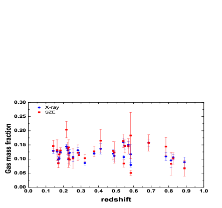
Figure 1: Gas mass fraction measurements as a function of redshift considered in our analysis (subsample of 29 galaxy clusters) La Roque (2006). Blue circles and red squares stand for measurements obtained from X-ray and SZE observations, respectively.

IV analysis and results

Recently, La Roque et al. La Roque (2006) provided a sample of measurements of the gas mass fraction of galaxy clusters from both X-ray and SZ observations. This sample, derived from Chandra X-ray observations and OVRO/BIMA interferometric Sunyaev-Zel’dovich Effect (SZE) measurements, comprises 38 $f_{gas}$ data points in the redshift interval $0.14\leq z\leq 0.89$. In their analysis, the authors used the nonisothermal double $\beta$-model for gas distribution and the 3D temperature profile was modelled assuming that the ICM is in hydrostatic equilibrium with a NFW dark matter density distribution Navarro and White (1997). The gas density model was obtained from a joint analysis of the X-ray and SZE data, which makes the SZE gas mass fraction not completely independent. However, Ref.  La Roque (2006) used $r_{2500}$ (the radius at which the mean enclosed mass density is equal to $2500$ cosmological critical density) in their analysis and current simulations Hallman (2007) have shown that the shape parameter values computed separately by SZE and X-ray observations agrees at $1\sigma$ level within this radius.

When described by the hydrostatic equilibrium model, some objects of the La Roque et al. sample presented questionable reduced $\chi^{2}$ ($2.43\leq\chi_{d.o.f.}^{2}\leq 41.62$). They are: Abell 665, ZW 3146, RX J1347.5-1145, MS 1358.4 + 6245, Abell 1835, MACS J1423+2404, Abell 1914, Abell 2163, Abell 2204. By excluding these objects from our analysis we end up with a subsample of 29 galaxy clusters, shown in Figure 1.

We evaluate our statistical analysis by defining the likelihood distribution function ${\cal{L}}\propto e^{-\chi^{2}/2}$, where

$$\chi^{2}=\sum_{i=1}^{N}\frac{{\left[1-\frac{1}{40}\beta_{had,0}{\phi_{0}^{\prime}}\ln{(1+z)}-\phi_{i,obs}(z)\right]}^{2}}{\sigma^{2}_{i,obs}},$$ (36)

$\phi_{i,obs}(z)=f_{SZE}/f_{X-ray}$ and $\sigma^{2}_{i,obs}$ is the uncertainty associated to this quantity, i. e.,

$$\sigma^{2}_{i,obs}=\left[\frac{1}{f_{X-ray}}\right]^{2}\sigma^{2}_{f_{SZE}}+\\ \left[\frac{f_{SZE}}{(f_{X-ray})^{2}}\right]^{2}\sigma^{2}_{f_{X-ray}}.$$

The error bars of gas mass fraction measurements take into account the statistical errors of the X-ray and SZE observations estimated in Ref. La Roque (2006). The common statistical contributions to $f_{gas}$ are: SZE point sources $\pm 4\%$, kinetic SZ $\pm 8\%$, $\pm 20\%$ and $\pm 10\%$ for cluster asphericity to $f_{gas}$ from X-ray and SZE observations, respectively. The asymmetric error bars were treated as discussed in D’Agostini (2004), i. e., $f_{gas}=\widetilde{f}_{gas}+\Delta_{+}-\Delta_{-}$, with $\sigma_{f_{gas}}=(\Delta_{+}+\Delta_{-})/2$, where $\widetilde{f}_{gas}$ stands for the La Roque et al. (2006) measurements and $\Delta_{+}$ and $\Delta_{-}$ are, respectively, the associated upper and lower errors bars. On the other hand, the systematic errors for the galaxy clusters are: X-ray absolute flux calibration $\pm 6\%$, X-ray temperature calibration $\pm 7.5\%$, SZE calibration $\pm 8\%$ and a one-sided systematic uncertainty of $-10\%$ to the total masses, which accounts for the assumed hydrostatic equilibrium. We also performed our analysis by combining the statistical and systematic errors in quadrature for the gas mass fractions of galaxy clusters.

Constraints on the quantity $\gamma=\frac{1}{40}\beta_{had,0}{\phi_{0}^{\prime}}$ are shown in Figure 2. Solid and dashed curves correspond to analyses with and without systematic errors, respectively. We obtain $\gamma=0.037\pm 0.18$ and $\gamma=0.065\pm 0.095$ at 68.3% (C.L.), which are fully compatible with $\phi(z)=1$ or, equivalently, with no variation of fine structure constant $\alpha$. Now, it is interesting to compare our bound on $\gamma$ with limits obtained using independent data. From the expression for the deceleration parameter $q_{0}$ and considering the Planck estimate for the total matter density $\Omega_{m}$, an upper bound on the value of $\phi_{0}^{\prime}$ can be estimated, namely, $\phi_{0}^{\prime}\leq 0.3$ at 1$\sigma$ c.l. Martins et al. (2015). Torsion balance tests and lunar laser ranging provide $\beta_{had,0}\leq 10^{-4}$ Wagner et al. (2012); Murphy (2013) whereas a comparison of atomic clocks with differente atomic number implies $\gamma\leq 3\times 10^{-5}$ Rosenband et al. (2008). It follows from this discussion, that the bounds obtained in this work from current $f_{gas}$ data, although less stringent, are fully consistent with limits obtained with independent data.

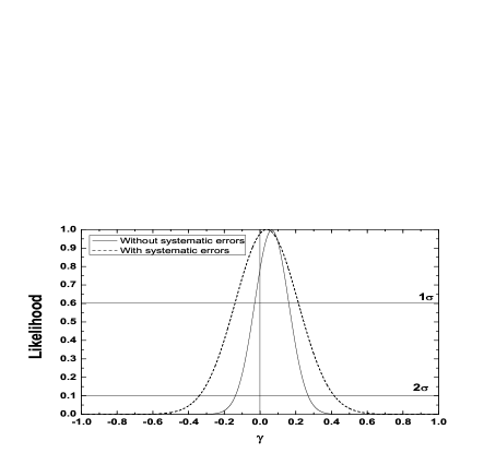
Figure 2: Constraints on a possible variation of the fine structure constant. The solid and dashed lines correspond to analyses with and without the systematic errors discussed in the text, respectively.

V Conclusions

The search for a possible variation of fundamental constants constitutes an important task not only for cosmology but also for fundamental physics (see, e.g., Langacker (2004)). In this work we have proposed a new method to investigate the time variation of the fine structure constant $\alpha$ in cosmological scales. We have shown that observations of the gas mass fraction via the Sunyaev-Zeldovich effect and X-ray surface brightness of the same galaxy cluster are related by $f_{SZE}=\varphi(z)f_{X-ray}$, where $\varphi(z)=\frac{\alpha}{\alpha_{0}}$, which furnishes constraints on the evolution of $\alpha$.

We have also applied such a method to a sample of 29 measurements of the gas mass fraction of galaxy clusters very well described by the hydrostatic equilibrium assumption, as discussed in Ref. La Roque (2006). Taking into account the results of Ref. Hees and Larena (2014), connecting variations of $\alpha$ with violation in the duality distance relation, we have derived, for a class of dilaton runaway models, new constraints on $\alpha$ which are fully compatible with $\phi(z)=1$. It is worth mentioning that a similar analysis using different galaxy cluster observables has been performed in Ref. Galli (2013). Differently from our results, however, the variation of $\alpha$ induced by the distance-duality relation was not considered in this latter work, which suggests that the bounds on $\alpha$ there derived should be revised. Given the small number of $f_{gas}$ data points currently available, the constraints reported here are not yet competitive with the tight bounds derived from other analises (see, e.g., Hees and Larena (2014) and references therein). We believe, however, that when applied to upcoming galaxy cluster data from current and planned surveys (e.g., SPT  and eROSITA ) the method discussed in this paper may be useful to probe a possible variation of the fine structure constant as well as to explore its theoretical consequences.

References

- Dirac (1937) P. A. M. Dirac, Nature 139, 323 (1937).
- Uzan (2003) J.-P. Uzan, Reviews of Modern Physics 75, 403 (2003), eprint hep-ph/0205340.
- Damour et al. (2002a) T. Damour, F. Piazza, and G. Veneziano, Physical Review Letters 89, 081601 (2002a).
- Uzan (2011) J.-P. Uzan, Living Reviews in Relativity 14 (2011), eprint 1009.5514.
- García-Berro et al. (2007) E. García-Berro, J. Isern, and Y. A. Kubyshin, Astron. Astrophys. Review 14, 113 (2007).
- Damour and Dyson (1996) T. Damour and F. Dyson, Nuclear Physics B 480, 37 (1996), URL http://adsabs.harvard.edu/cgi-bin/nph-bib_query?bibcode=1996NuPhB.480...37D&db_key=PHY.
- Petrov et al. (2006) Y. V. Petrov, A. I. Nazarov, M. S. Onegin, V. Y. Petrov, and E. G. Sakhnovsky, Physical Review C 74, 064610 (2006), eprint arXiv:hep-ph/0506186.
- Gould et al. (2006) C. R. Gould, E. I. Sharapov, and S. K. Lamoreaux, Physical Review C 74, 024607 (2006), eprint arXiv:nucl-ex/0701019.
- Onegin et al. (2012) M. S. Onegin, M. S. Yudkevich, and E. A. Gomin, Modern Physics Letters A 27, 1250232 (2012), eprint 1010.6299.
- Fischer et al. (2004) M. Fischer, N. Kolachevsky, M. Zimmermann, R. Holzwarth, T. Udem, T. W. Hänsch, M. Abgrall, J. Grünert, I. Maksimovic, S. Bize, et al., Physical Review Letters 92, 230802 (2004).
- Peik et al. (2004) E. Peik, B. Lipphardt, H. Schnatz, T. Schneider, C. Tamm, and S. G. Karshenboim, Physical Review Letters 93, 170801 (2004), eprint physics/0402132.
- Rosenband et al. (2008) T. Rosenband, D. B. Hume, P. O. Schmidt, C. W. Chou, A. Brusch, L. Lorini, W. H. Oskay, R. E. Drullinger, T. M. Fortier, J. E. Stalnaker, et al., Science 319, 1808 (2008).
- Adelberger et al. (2009) E. G. Adelberger, J. H. Gundlach, B. R. Heckel, S. Hoedl, and S. Schlamminger, Progress in Particle and Nuclear Physics 62, 102 (2009).
- Wagner et al. (2012) T. A. Wagner, S. Schlamminger, J. H. Gundlach, and E. G. Adelberger, Classical and Quantum Gravity 29, 184002 (2012), eprint 1207.2442.
- Murphy (2013) T. W. Murphy, Reports on Progress in Physics 76, 076901 (2013), eprint 1309.6294.
- Kraiselburd and Vucetich (2012) L. Kraiselburd and H. Vucetich, Physics Letters B 718, 21 (2012), eprint 1110.3527.
- Webb et al. (1999) J. K. Webb, V. V. Flambaum, C. W. Churchill, M. J. Drinkwater, and J. D. Barrow, Physical Review Letters 82, 884 (1999), URL http://adsabs.harvard.edu/cgi-bin/nph-bib_query?bibcode=1999PhRvL..82..884W&db_key=PHY.
- Webb et al. (2003) M. T. Webb, J.K.and Murphy, V. V. Flambaum, and S. J. Curran, Astrophys. Space Science 283, 577 (2003).
- King et al. (2012) J. A. King, J. K. Webb, M. T. Murphy, V. V. Flambaum, R. F. Carswell, M. B. Bainbridge, M. R. Wilczynska, and F. E. Koch, MNRAS 422, 3370 (2012), eprint 1202.4758.
- Whitmore and Murphy (2015) J. B. Whitmore and M. T. Murphy, MNRAS 447, 446 (2015), eprint 1409.4467.
- O’Bryan et al. (2015) J. O’Bryan, J. Smidt, F. De Bernardis, and A. Cooray, Astrophys. J. 798, 18 (2015).
- Planck Collaboration et al. (2014) Planck Collaboration, P. A. R. Ade, N. Aghanim, M. Arnaud, M. Ashdown, J. Aumont, C. Baccigalupi, A. J. Banday, R. B. Barreiro, E. Battaner, et al., ArXiv e-prints (2014), eprint 1406.7482.
- Mosquera and Civitarese (2013) M. E. Mosquera and O. Civitarese, Astron. and Astrophys. 551, A122 (2013).
- Galli (2013) S. Galli, Phys. Rev. D 87, 123516 (2013), eprint 1212.1075.
- Hees and Larena (2014) O. Hees, A. Minazzoli and J. Larena, PRD 90, 124064 (2014).
- La Roque (2006) S. J. e. a. La Roque, ApJ 652, 917 (2006).
- Bekenstein (1982) J. D. Bekenstein, Phys. Rev. D 25, 1527 (1982).
- Barrow et al. (2002) J. D. Barrow, J. Magueijo, and H. B. Sandvik, Phys. Rev. D 66, 043515 (2002).
- Olive et al. (2002) K. A. Olive, M. Pospelov, Y. Qian, A. Coc, M. Cassé, and E. Vangioni-Flam, Phys. Rev. D 66, 045022 (2002).
- Damour and Polyakov (1994) T. Damour and A. M. Polyakov, Nuclear Physics B 423, 532 (1994), eprint arXiv:hep-th/9401069.
- Damour et al. (2002b) T. Damour, F. Piazza, and G. Veneziano, Phys. Rev. D 66, 046007 (2002b).
- Martins et al. (2015) C. J. A. P. Martins, P. E. Vielzeuf, M. Martinelli, E. Calabrese, and S. Pandolfi, ArXiv e-prints (2015), eprint 1503.05068.
- Khoury and Weltman (2004) J. Khoury and A. Weltman, Physical Review Letters 93, 171104 (2004), eprint astro-ph/0309300.
- Brax et al. (2004) P. Brax, C. van de Bruck, A.-C. Davis, J. Khoury, and A. Weltman, Phys. Rev. D 70, 123518 (2004), eprint astro-ph/0408415.
- Mota and Shaw (2007) D. F. Mota and D. J. Shaw, Phys. Rev. D 75, 063501 (2007), eprint hep-ph/0608078.
- Kraiselburd et al. (2014) L. Kraiselburd, S. Landau, M. Salgado, and D. Sudarsky, Memorie della Societa Astronomica Italiana 85, 32 (2014), eprint 1310.6051.
- Sasaki (1996) S. Sasaki, PASJ 48 (1996).
- Cavaliere and Fusco-Fermiano (1978) A. Cavaliere and R. Fusco-Fermiano, Astron. and Astrophys. 667, 70 (1978).
- Grego (2001) L. e. a. Grego, ApJ 552, 2 (2001).
- Sarazin (1986) C. L. Sarazin, ApJ 1, 300 (1986).
- Holanda and Alcaniz (2012) R. S. Holanda, R. F. L. Goncalves and J. S. Alcaniz, JCAP 1206, 022 (2012).
- Sunyaev and Zeldovich (1972) R. A. Sunyaev and Y. B. Zeldovich, Comments Astrophys. Space Phys. 4, 173 (1972).
- Itoh and Nozawa (1998) Y. Itoh, N. Kohyama and S. Nozawa, ApJ 502, 7 (1998).
- Navarro and White (1997) C. S. Navarro, J. F. Frenk and S. D. M. White, ApJ 490, 493 (1997).
- Hallman (2007) E. J. e. a. Hallman, ApJ 665, 911 (2007).
- D’Agostini (2004) G. D’Agostini, arxiv:0403086 (2004).
- Langacker (2004) P. Langacker, International Journal of Modern Physics A 19, 157 (2004), eprint hep-ph/0304093.