Duality relation for a generalized interferometer

Abstract

It is well known that the Mach-Zender interferometer exhibits a trade-off between the a priori which-path knowledge and the visibility of its interference pattern. This trade-off is expressed by the inequality $\mathcal{P}^{2}+\mathcal{V}^{2}\leq 1$, constraining the predictability $\mathcal{P}$ and visibility $\mathcal{V}$ of the interferometer. In this paper we extend the Mach-Zender scheme to a setup where the central phase shifter is substituted by a generic unitary operator. We find that the sum $\mathcal{P}^{2}+\mathcal{V}^{2}$ is in general no longer upper bounded by $1$, and that there exists a whole class of interferometers such that the full fringe visibility and the full which-way information are not mutually exclusive. We show that $\mathcal{P}^{2}+\mathcal{V}^{2}\leq L_{U}$, with $1\leq L_{U}\leq 2$, and we illustrate how the tight bound $L_{U}$ depends on the choice of the unitary operation $U$ replacing the central phase shifter.

I Introduction

One of the most distinctive aspects of quantum mechanics is the possibility to adopt two different perspectives which separately highlight the particle-like and wave-like nature of the same system. Moreover, Bohr’s complementarity principle states that the two descriptions are mutually exclusive, in that it is not possible to perform an experiment which allows the system to exhibit both its particle and wave properties at the same time Bohr (1928). The most famous demonstration of this principle is Young’s double-slit experiment, where a beam of particles individually fired through two slits generates a density distribution on the detection screen which corresponds to the interference pattern that would be created by a wave. Yet when one tries to determine through which slit each particle has passed, the interference pattern is inevitably wiped out. This characteristic is known as “wave-particle duality”.

However a quantitative formulation of this principle was first derived only in 1979 by Wootters and Zurek Wootters and Zurek (1979): by analysing Einstein’s version of the double-slit experiment, they found that it is possible to gain partial knowledge of a single photon’s path without erasing the interference pattern. The result was also obtained by Bartell Bartell (1980) with two alternative variations of the same apparatus. Greenberger and Yasin extended the analysis to the case of a two-way neutron interferometer Greenberger and Yasin (1988), and introduced two relevant quantities that will be adopted in the present work: the predictability $\mathcal{P}$ and the fringe visibility $\mathcal{V}$. The trade-off between the amount of “path information” and the interference sharpness can then be expressed as a constraint on $\mathcal{P}$ and $\mathcal{V}$ in the form of an inequality:

$$\mathcal{P}^{2}+\mathcal{V}^{2}\leq 1,$$ (1)

which can be saturated only by some pure states Englert (1996).

Interferometric dualities have been intensively studied in the last decades Jaeger et al. (1993, 1995); Englert (1996); Englert and Bergou (2000); Martinez-Linares and Harmin (2004); Luis (2004); Englert et al. (2008); Erez et al. (2009); Liu et al. (2009); Li et al. (2012); Coles et al. (2014); Jia et al. (2014); Bera et al. (2015): in these works the predictability, which is based solely on the knowledge of the preparation of the initial state, is often substituted by another quantity, the “distinguishability”Englert (1996), expressing the degree of which-way information acquired after the particle has interacted with auxiliary detectors Jaeger et al. (1993, 1995); Englert (1996); Englert and Bergou (2000); Martinez-Linares and Harmin (2004); Erez et al. (2009). These dualities have also been interpreted as constraints over the joint measurement of pairs of unsharp observables Liu et al. (2009); Li et al. (2012) and recently it has been argued that all of them are in fact particular cases of more general entropic uncertainty relations Coles et al. (2014). Experimental validations of both kinds of dualities have been performed with neutron Rauch and Summhammer (1984); Summhammer et al. (1987) and optical Liu et al. (2012); Tang et al. (2013); Yan et al. (2015); Heuer et al. (2015) interferometers, and by various implementations of Wheeler’s “delayed choice” experiment Jacques et al. (2007, 2008); Manning et al. (2015).

It is interesting to notice that while wave-particle duality is usually considered an inherently quantum feature, there is also evidence of interference effects in the diffraction of large molecules such as fullerenes Arndt et al. (1999). But interference has been observed at a much larger scale: a macroscopic droplet bouncing on a vibrating bath can generate a field of surface waves that couples with it. The field acts as a pilot wave guiding the droplet as it moves steadily over the surface Couder et al. (2005). Couder and Fort have shown that, when these “walkers” pass through a double-slit screen, the distribution of their scattered trajectories matches the interference pattern of the diffracted pilot waves Couder and Fort (2006). Furthermore, due the large scale of the droplets ($\sim 1\mathrm{mm}$) it is possible to observe simultaneously both their path and the interference of their guiding waves. These striking similarities between the walkers’ behaviour and the quantum wave-particle duality leave open the question whether the macroscopic (classical) and microscopic (quantum) worlds are really so different, or if the former can provide some insight into the latter Bush (2010).

To investigate further the nature of wave-particle duality, here we want to study an extension of the Mach-Zender interferometric setup Englert (1996), where the particular unitary operator representing the middle phase shifter is replaced by an generic unitary $U$. We find that in this situation the sum $\mathcal{P}^{2}+\mathcal{V}^{2}$ can assume all values in the range $[0,2]$. In particular we will show that

$$\mathcal{P}^{2}+\mathcal{V}^{2}\leq L_{U},$$ (2)

where $L_{U}$, the maximum value of $\mathcal{P}^{2}+\mathcal{V}^{2}$ taken over all the possible input states, depends on the choice of the middle unitary $U$, and $1\leq L_{U}\leq 2$. As a consequence the trade-off between the so called “particle-like” and “wave-like” behaviours disappears. We will also show that the transition between the two extremal values is smoothly dependent on the parameters of the unitary.

This article is structured as follows: in section II we briefly describe the Mach-Zender interferometer and the meaning of the two relevant quantities $\mathcal{P}$ and $\mathcal{V}$. In section III we introduce a generalized interferometer by replacing the middle phase shifter with a generic unitary and in this new scheme we identify the expressions for predictability and visibility. In section IV we show that the generalized setup satisfies the relation (2), with $1\leq L_{U}\leq 2$. In section V we illustrate the smooth dependence of $L_{U}$ on the physical parameters of our setup and we interpret the generalized middle unitary in terms of linear optical transformations. In the last section we discuss the results and their implications.

II The Mach-Zender interferometer

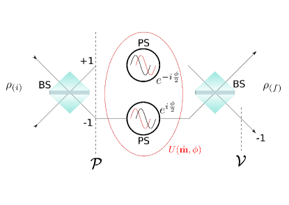
Figure 1: Illustration of the Mach-Zender (M-Z) interferometer as described in Englert (1996): after the action of the first beam splitter, a differential phase $\phi$ is applied to the two arms by two phase shifters (PS) and the beams are then crossed again by another beam splitter. In the generalized setup, the phase shifters are replaced by a generic unitary $U$ which is determined by its rotation axis $\hat{\mathbf{m}}$ and by the angle $\phi$ (Eq. (8)). The predictability $\mathcal{P}$ (Eq. (6)) is calculated after the first BS, while the fringe visibility $\mathcal{V}$ (Eq. (7)) quantifies the sharpness of the interference pattern obtained at the end of the process when varying $\phi$.

In the standard Mach-Zender interferometer (see Fig. 1), a particle sent through a 50:50 beam splitter (BS) can take either of two paths. The path is the relevant degree of freedom, therefore there are two modes, corresponding to the two paths, and the particle can be effectively described as a $2$-level system. Identifying the “which-way” observable with the Pauli matrix $\sigma_{z}$ the Hilbert space is spanned by its two eigenstates: $\Ket{0}$ and $\Ket{1}$. Their eigenvalues, $+1$ and $-1$, label the two paths. A convenient representation of the BS is given by the unitary operator $e^{-i\frac{\pi}{4}\sigma_{y}}=\frac{1}{\sqrt{2}}\left(\mathbf{1}-i\sigma_{y}\right)$, which maps the path-eigenstates $\Ket{0}$, $\Ket{1}$ onto their equal superpositions $\Ket{\pm}=(\Ket{0}\pm\Ket{1})/\sqrt{2}$:

$$\begin{split}e^{-i\frac{\pi}{4}\sigma_{y}}\Ket{0}=\frac{\mathbf{1}-i\sigma_{y}}{\sqrt{2}}\Ket{0}=\frac{\Ket{0}+\Ket{1}}{\sqrt{2}},\\ e^{-i\frac{\pi}{4}\sigma_{y}}\Ket{1}=\frac{\mathbf{1}-i\sigma_{y}}{\sqrt{2}}\Ket{1}=\frac{\Ket{0}-\Ket{1}}{\sqrt{2}}.\end{split}$$

Generally the system will be initially prepared in a mixed state, represented by the density matrix

$$\rho_{(i)}=\frac{\mathbf{1}+\mathbf{s}_{(i)}\cdot\hat{\mathbf{\sigma}}}{2},$$ (3)

with Bloch vector $\mathbf{s}_{(i)}$, and where $\hat{\mathbf{\sigma}}\equiv(\sigma_{x},\sigma_{y},\sigma_{z})$ is the triple of Pauli’s matrices.

The Bloch vector representing the system’s state after the action of the first BS is then

$$\mathbf{s}_{1}=\hat{\mathbf{e}}_{y}\times\mathbf{s}_{(i)}+s_{(i)y}\hat{\mathbf{e}}_{y}.$$ (4)

This formula has a straightforward geometric interpretation: $\mathbf{s}_{(i)}$ is rotated by an angle $\pi/2$ about the direction $\hat{\mathbf{e}}_{y}$ in the Bloch sphere.

In Englert (1996) the which-way predictability was defined as the a priori knowledge of the path taken by the particle after it has passed through the beam splitter. The probabilities $w_{\pm}$ of getting the values $\pm 1$ upon the measurement of the $\sigma_{z}$ observable, are given by

$$w_{\pm}=\mathrm{Tr}\left[\frac{\mathbf{1}\pm\sigma_{z}}{2}\left(e^{-i\frac{\pi}{4}\sigma_{y}}\frac{\mathbf{1}+\mathbf{s}_{(i)}\cdot\hat{\mathbf{\sigma}}}{2}e^{i\frac{\pi}{4}\sigma_{y}}\right)\right]=\frac{1\pm s_{1z}}{2}.$$ (5)

The predictability is then defined by

$$\mathcal{P}=\lvert w_{+}-w_{-}\rvert=|s_{1z}\rvert=\lvert s_{(i)x}\rvert.$$ (6)

$\mathcal{P}$ estimates the ability to make a correct guess of the path that will be taken. In particular, $\mathcal{P}=1$ corresponds to a full a priori knowledge of the path and it is therefore associated to a particle-like behaviour (in the classical sense of a system having a definite trajectory).

After the action of the BS two phase shifters (PS) apply a differential phase $\phi$ to the two beams, which are then crossed by a second BS, identical to the first. Finally, a detector determines whether the particle takes a given exit path, e.g. the one labeled by $-1$. The interaction with the detector corresponds to an actual measurement of the observable $\sigma_{z}$. The procedure is repeated many times, starting with the same input state $\rho_{(i)}$. Upon a large number of measurements of $\sigma_{z}$ the frequency of the outcome $-1$ is obtained. This frequency $p$ depends on the applied differential phase $\phi$. The dependence $p=p(\phi)$ can be reconstructed by performing a set of many measurement of $\sigma_{z}$ for different values of $\phi$. As a final result $p(\phi)$ exhibits a sinusoidal profile Englert (1996). The contrast of its oscillations is quantified by the fringe visibility $\mathcal{V}$, defined as the ratio between the amplitude of the oscillations and its average value or, equivalently, if $I_{\mathrm{max}}$ and $I_{\mathrm{min}}$ are the maximum and minimum intensity, as

$$\mathcal{V}=\frac{I_{\mathrm{max}}-I_{\mathrm{min}}}{I_{\mathrm{max}}+I_{\mathrm{min}}}.$$ (7)

From their definitions it is clear that the quantities $\mathcal{P}$ and $\mathcal{V}$ can assume values in the range $[0,1]$. Nevertheless it turns out that they are constrained by the inequality (1), which includes all the intermediate situations between the full-defined interferometric pattern of the pure wave-like case (corresponding to the maximum visibility $\mathcal{V}=1$) and the full which-way information of the particle-like case ($\mathcal{P}=1$).

In particular it can be shown that $\mathcal{P}^{2}+\mathcal{V}^{2}=\lvert\mathbf{s}_{(i)}|^{2}$ (see for example Englert (1996)), and therefore the inequality (1) is saturated only by pure input states, which have $\lvert\mathbf{s}_{(i)}|^{2}=1$.

III Generalized interferometer

Inspired by the Mach-Zehnder interferometer here we consider an alternative scheme where the phase shifter $e^{-i\frac{\phi}{2}\sigma_{z}}$ is replaced by a general unitary transformation (see Fig. 1)

$$U=e^{-i\hat{\mathbf{m}}\cdot\hat{\mathbf{\sigma}}\,\phi/2}.$$ (8)

Here the rotation axis is determined by the unit vector $\hat{\mathbf{m}}$ and the rotation angle given by $\phi$. We also implement the second BS with the inverse of the first one, that is $e^{i\sigma_{y}\pi/4}$. With this choice, in absence of any middle transformation, $\sigma_{z}$’s eigenstates are mapped back into themselves.

The system’s state now undergoes the overall unitary $V\equiv e^{i\frac{\pi}{4}\sigma_{y}}Ue^{-i\frac{\pi}{4}\sigma_{y}}$, which can be written as a function of the parameters $\phi$ and $\hat{\mathbf{m}}$:

$$V=e^{-i\frac{\phi}{2}(-m_{z}\sigma_{x}+m_{y}\sigma_{y}+m_{x}\sigma_{z})}=e^{-i\mathbf{t}\cdot\hat{\sigma}\frac{\phi}{2}},$$ (9)

where the $3$-dimensional unit vector $\mathbf{t}(\hat{\mathbf{m}})$ takes the form

$$\mathbf{t}(\hat{\mathbf{m}})=-m_{z}\hat{\mathbf{e}}_{x}+m_{y}\hat{\mathbf{e}}_{y}+m_{x}\hat{\mathbf{e}}_{z}.$$ (10)

The final state

$$\rho_{(f)}=V\rho_{(i)}V^{\dagger}=\frac{\mathbf{1}+\mathbf{s}_{(f)}\cdot\hat{\mathbf{\sigma}}}{2},$$ (11)

is then determined by the Bloch vector

$$\mathbf{s}_{(f)}=\cos\phi\,\mathbf{s}_{(i)}+\sin\phi\,(\mathbf{t}\times\mathbf{s}_{(i)})+(1-\cos\phi)\,(\mathbf{t}\cdot\mathbf{s}_{(i)})\mathbf{t}.$$ (12)

After the qubit has passed through the second BS, the path measurement $\sigma_{z}$ is finally performed. The probability of getting one of the two outcomes, say $-1$, is the expectation value of the projector $(\mathbf{1}-\sigma_{z})/2$ evaluated on the final state $\mathbf{\rho}_{(f)}$:

$$p=\mathrm{Tr}\left[\left(\frac{\mathbf{1}-\sigma_{z}}{2}\right)\left(\frac{\mathbf{1}+\mathbf{s}_{(f)}\cdot\hat{\mathbf{\sigma}})}{2}\right)\right].$$ (13)

By using (12), this probability can be expressed as a function of the phase $\phi$ applied by the unitary $U$:

$$\begin{split}p=p(\phi)=\frac{1}{2}&\Big{\{}1-(\mathbf{t}\cdot\mathbf{s}_{(i)})t_{z}-\left[s_{(i)z}-(\mathbf{t}\cdot\mathbf{s}_{(i)})t_{z}\right]\cos\phi\\ &-\left[(\mathbf{t}\times\mathbf{s}_{(i)})_{z}\right]\sin\phi\Big{\}}.\end{split}$$ (14)

The visibility of a sinusoidal interferometric pattern is defined as in (7), which leads to the following result :

$$\mathcal{V}=\sqrt{\frac{\left[s_{(i)z}-(\mathbf{t}\cdot\mathbf{s}_{(i)})t_{z}\right]^{2}+\left[(\mathbf{t}\times\mathbf{s}_{(i)})_{z}\right]^{2}}{\left[1-(\mathbf{t}\cdot\mathbf{s}_{(i)})t_{z}\right]^{2}}}.$$ (15)

So far the quantities $\mathcal{P}$ and $\mathcal{V}$ have been derived in the most general case, where no assumption has been made on the vector $\hat{\mathbf{m}}$ appearing in (8). In the following section we show that the sum $\mathcal{P}^{2}+\mathcal{V}^{2}$ is crucially dependent on the mutual orientation of $\hat{\mathbf{e}}_{y}$ and $\hat{\mathbf{m}}$ (i.e. of the vectors defining the BS unitary and the middle unitary, respectively) as well as on the angle between $\hat{\mathbf{m}}$ and $\hat{\mathbf{e}}_{z}$, which is the axis identifying the “which-path” observable. In particular, the inequality (1) is no longer valid in the generalized interferometer.

IV Duality relation

First, we briefly discuss a trivial case for the system’s input state, i.e. the totally depolarized state $\rho_{(i)}=\mathbf{1}/2$, corresponding to $\mathbf{s}_{(i)}=0$. If $\mathbf{s}_{(i)}=0$ the system’s state remains unaltered under any unitary, therefore $\mathbf{s}_{1}=0$ and $\mathbf{s}_{(f)}=0$ imply that both the predictability (6) and the probability $p(\phi)$ (14) vanish. As one would expect for the maximally entropic state, one obtains $\mathcal{P}^{2}+\mathcal{V}^{2}=0$.

Another interesting case is the pure input state $\mathbf{s}_{(i)}=\hat{\mathbf{e}}_{z}$. This is mapped by the BS onto the Bloch vector $\hat{\mathbf{e}}_{x}$, whose density matrix represents the projector onto a 50:50 superposition of the two which-way eigenstates, that is $(\Ket{0}+\Ket{1})/\sqrt{2}$. Therefore, in agreement with Eq. (6), $\mathcal{P}=0$. It is easy to check that the visibility instead is $\mathcal{V}=1$.

Here we want to show that our generalized setup implies that, in a large number of cases, the sum $\mathcal{P}^{2}+\mathcal{V}^{2}$ can be higher than $1$ and, in fact, it can easily reach its maximum value $2$. In order to simplify our analysis we pick now as initial states the Bloch vectors $\mathbf{s}_{(i)}=s_{x}\hat{\mathbf{e}}_{x}$, with $0\leq s_{x}\leq 1$. As they are mapped onto the $z$-axis, the predictability can assume any value from $0$ to $1$.

The unit vector $\hat{\mathbf{m}}$ can be decomposed into its projected component $\mathbf{m}_{P}$ on the $(x,y)$ plane and the orthogonal component $\mathbf{m}_{\perp}$ (see Fig. 2); then it can be written in spherical coordinates:

$$\hat{\mathbf{m}}=\mathbf{m}_{\perp}+\mathbf{m}_{P}=\cos\Theta\,\hat{\mathbf{e}}_{z}+\sin\Theta\left(\cos\xi\,\hat{\mathbf{e}}_{x}+\sin\xi\,\hat{\mathbf{e}}_{y}\right).$$ (16)

In this way we can express $\mathcal{P}^{2}+\mathcal{V}^{2}$ in spherical coordinates through (6), (15) and (16). We call this function $F$:

$$F(s_{x},\Theta,\xi)=\lvert s_{x}\rvert^{2}\left(1+\frac{\sin^{2}\Theta(\cos^{2}\Theta\cos^{2}\xi+\sin^{2}\xi)}{(1+s_{x}\sin\Theta\cos\Theta\cos\xi)^{2}}\right),$$ (17)

and notice that it spans the whole range of values $0\leq F\leq 2$.

If we take as input the pure state $\mathbf{s}_{(i)}=\hat{\mathbf{e}}_{x}$ then the sum will assume the simpler form:

$$F(1,\Theta,\xi)=\left(1+\frac{\sin^{2}\Theta\cos^{2}\Theta\cos^{2}\xi+\sin^{2}\Theta\sin^{2}\xi}{(1+\sin\Theta\cos\Theta\cos\xi)^{2}}\right).$$ (18)

In Fig. 3 this function is plotted. It is evident that the inequality

$$\mathcal{P}^{2}+\mathcal{V}^{2}\leq 2$$ (19)

is saturated for a variety of different orientations of the vector $\hat{\mathbf{m}}$. Moreover, both the inequalities (1) and (19) can only be saturated by the two input states $\mathbf{s}_{(i)}=\pm\hat{\mathbf{e}}_{x}$, since the predictability is given by $\mathcal{P}=\lvert\mathbf{s}_{(i)}\cdot\hat{\mathbf{e}}_{x}\rvert$.

It is interesting to observe what condition on $\hat{\mathbf{m}}$ determines an upper bound equal to $1$: the second term in (17) vanishes if either $\Theta\in\{0,\pi\}$, which means that $\hat{\mathbf{m}}=\pm\hat{\mathbf{e}}_{z}$ and therefore the unitary $U=e^{-i\phi\sigma_{z}/2}$ is a phase shifter as in Englert (1996), or if $\xi=0$ and $\cos\Theta=0$, which means $\hat{\mathbf{m}}=\pm\hat{\mathbf{e}}_{x}$, that is if the central unitary is another beam splitter: $U=e^{-i\phi\sigma_{x}/2}$.

However, orthogonality between the two unit vectors $\hat{\mathbf{m}}$ and $\hat{\mathbf{e}}_{y}$ is not sufficient to ensure that $\mathcal{P}^{2}+\mathcal{V}^{2}\leq 1$ in this scenario, since one can take $\hat{\mathbf{m}}$ in the plane $(x,z)$ such that $F\geq 1$: e.g. if $\hat{\mathbf{m}}=(\hat{\mathbf{e}}_{x}+\hat{\mathbf{e}}_{z})/\sqrt{2}$, then $\Theta=\pi/4$, $\xi=0$ imply $F(s_{x},\Theta,\xi)=\lvert s_{x}\rvert^{2}(1+1/(2+s_{x})^{2})$ which is larger than $1$ for the pure state $\mathbf{s}_{(i)}=\hat{\mathbf{e}}_{x}$. The reason is that, unlike the Mach-Zender interferometer analysed in Englert (1996), the observable which is being measured, $\sigma_{z}$, is now different from the operator $\hat{\mathbf{m}}\cdot\hat{\mathbf{\sigma}}$ defining the unitary $U$.

The duality relation (19) has an important consequence: if one considers generalized interferometric setups, where the middle unitary is not a phase-shifter, then it is possible to achieve a perfect which-way knowledge ($\mathcal{P}=1$) without destroying the interference pattern ($\mathcal{V}\neq 0$). And viceversa: a full fringe visibiliy ($\mathcal{V}=1$) is no longer incompatible with a high degree of predictability.

Figure 2: The decomposition of the unit vector $\hat{\mathbf{m}}$ into its projection $\mathbf{m}_{P}$ onto the plane $(x,y)$ and its orthogonal component $\mathbf{m}_{\perp}$. The visibility can be expressed as a function of the polar variables $\Theta$ and $\xi$.

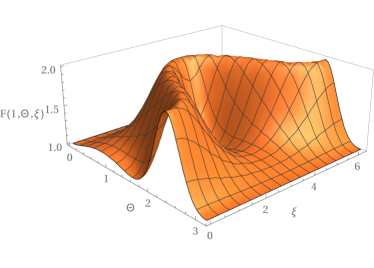
Figure 3: Plot of the function $F(1,\Theta,\xi)=\mathcal{P}^{2}+\mathcal{V}^{2}$ corresponding to the choice $\mathbf{s}_{(i)}=\hat{\mathbf{e}}_{x}$. Here $\Theta$ is the angle between the vectors $\hat{\mathbf{m}}$ and $\hat{\mathbf{e}}_{z}$, and $\xi$ the angle between $\hat{\mathbf{e}}_{x}$ and the projection $\mathbf{m}_{P}$ of $\hat{\mathbf{m}}$ on the plane $(x,y)$. There are configurations of the vector $\hat{\mathbf{m}}$ such that the quantity $F=\mathcal{P}^{2}+\mathcal{V}^{2}$ can be larger than $1$.

V Variation of the inequality’s upper bound

In order to illustrate the dependence of the visibility (15) on the mutual orientation of $\hat{\mathbf{e}}_{y}$ and $\hat{\mathbf{m}}$, we consider again the pure initial state $\mathbf{s}_{(i)}=\hat{\mathbf{e}}_{x}$ and recast the sum $\mathcal{P}^{2}+\mathcal{V}^{2}$ in terms of the $(x,y,z)$ coordinates of the vector $\hat{\mathbf{m}}$. From Eq. (16)

$$m_{x}=\sin\Theta\cos\xi,\quad m_{y}=\sin\Theta\sin\xi,\quad m_{z}=\cos\Theta.$$ (20)

Therefore Eq. (18) can be rewritten, reminding that $\hat{\mathbf{m}}$ is a unit vector ($m_{x}^{2}+m_{y}^{2}+m_{z}^{2}=1$), as a function of $m_{x}$ and $m_{z}$:

$$\mathcal{P}^{2}+\mathcal{V}^{2}=f(m_{x},m_{z})\equiv\left[1+\frac{(1-m_{x}^{2})(1-m_{z}^{2})}{(1+m_{z}m_{x})^{2}}\right].$$ (21)

It can be shown that this function has no local isolated extremal points but it assumes its maximum value $1$ on the line $m_{z}=-m_{x}$ (see Fig. 5). On the other hand, if we restrict the study of $f(m_{x},m_{z})$ to the subdomain $\mathcal{L}=\{(m_{x},m_{x}):m_{x}\in[0,\frac{1}{\sqrt{2}}]\}$, the profile of the one-dimensional function $[0,\frac{1}{\sqrt{2}}]\ni m_{x}\mapsto f(m_{x},m_{x})$ is monotonic with maximum and mininum values $2$ and $\frac{10}{9}$. In Fig. 5 this profile is shown in red.

A suitable change of coordinates provides a more vivid picture of the mentioned transition (see Fig. 4): upon a $-45^{\circ}$ rotation about the $y$ axis the orthonormal basis $(\hat{\mathbf{e}}_{x},\hat{\mathbf{e}}_{y},\hat{\mathbf{e}}_{z})$ is mapped onto

$$\hat{\mathbf{e}}_{x^{\prime}}=\frac{\hat{\mathbf{e}}_{x}+\hat{\mathbf{e}}_{z}}{\sqrt{2}},\quad\hat{\mathbf{e}}_{y^{\prime}}=\hat{\mathbf{e}}_{y},\quad\hat{\mathbf{e}}_{z^{\prime}}=\frac{-\hat{\mathbf{e}}_{x}+\hat{\mathbf{e}}_{z}}{\sqrt{2}}.$$ (22)

In this coordinates system the $1$-dimensional manifold $\mathcal{L}$ is parametrized as $\mathcal{L}=\{(m_{x^{\prime}},0):m_{x^{\prime}}\in[0,1]\}$. As the $m_{x^{\prime}}$ component varies from $0$ to $1$, the unit vector $\hat{\mathbf{m}}$ rotates from $\hat{\mathbf{e}}_{y}$ to $\hat{\mathbf{e}}_{x^{\prime}}$: $\hat{\mathbf{m}}\equiv\hat{\mathbf{e}}_{y}$ means that the overall unitary operator (9) is actually equivalent to $U$ and the visibility is at its maximum, $1$, while when the two vectors $\hat{\mathbf{m}}$ and $\hat{\mathbf{e}}_{y}$ are orthogonal ($m_{x^{\prime}}=1$) then the fringe pattern assumes its minimum.

We can also reintroduce the dependence on the initial state $\mathbf{s}_{(i)}=s_{x}\hat{\mathbf{e}}_{x}$ as in (17). In the new parameters $F$ will become a function $\tilde{f}(s_{x},m_{x^{\prime}})$ of $s_{x}$ and $m_{x}^{\prime}$:

$$\tilde{f}(s_{x},m_{x^{\prime}})=\mathcal{P}^{2}(s_{x})+\mathcal{V}^{2}(s_{x},m_{x^{\prime}})=\\ s_{x}^{2}+s_{x}^{2}\frac{\left(1-(\frac{m_{x^{\prime}}}{\sqrt{2}})^{2}\right)^{2}}{\left(1+s_{x}(\frac{m_{x^{\prime}}}{\sqrt{2}})^{2}\right)^{2}}.$$ (23)

$\tilde{f}(s_{x},m_{x^{\prime}})$is plotted in Fig. 6 for different values of $s_{x}$.

So far we have considered 50:50 BS represented by the unitary $e^{-i\pi\sigma_{y}/4}$. One can generalize it to an operator of the form $e^{-i\omega\sigma_{y}/2}$. The angle $\omega$ can now vary, and any value other than $\pi/2$ corresponds to an unbalanced BS. In fact, if $t_{\pm}$ and $r_{\pm}$ are the transmissivity and reflectivity coefficients, then the unitary

$$e^{-i\frac{\omega}{2}\sigma_{y}}=\begin{pmatrix}t_{+}(\omega)&r_{-}(\omega)\\ r_{+}(\omega)&t_{-}(\omega)\end{pmatrix}=\begin{pmatrix}\cos\frac{\omega}{2}&-\sin\frac{\omega}{2}\\ \sin\frac{\omega}{2}&\cos\frac{\omega}{2}\end{pmatrix},$$ (24)

maps the initial state represented by the Bloch vector $\hat{\mathbf{s}}_{(i)}$ onto a state represented by

$$\hat{\mathbf{s}}_{1}=\cos\omega\hat{\mathbf{s}}_{(i)}+\sin\omega(\hat{\mathbf{e}}_{y}\times\hat{\mathbf{s}}_{(i)})+(1-\cos\omega)s_{(i)y}\hat{\mathbf{e}}_{y}.$$ (25)

Figure 4: The vector $\hat{\mathbf{m}}$ is restricted to the $(\hat{\mathbf{e}}_{y},\hat{\mathbf{e}}_{x^{\prime}})$ plane. This constraint simplifies the discussion and allows an immediate display of the transition from a situation, $\hat{\mathbf{m}}\perp\hat{\mathbf{e}}_{y}$, where the quantity $\mathcal{P}^{2}+\mathcal{V}^{2}$ assumes its minimum (but it is still greater than 1) to a situation, $\hat{\mathbf{m}}\parallel\hat{\mathbf{e}}_{y}$, where the the full knowledge of both observables at the same time is allowed ($\mathcal{P}^{2}+\mathcal{V}^{2}\leq 2$) .

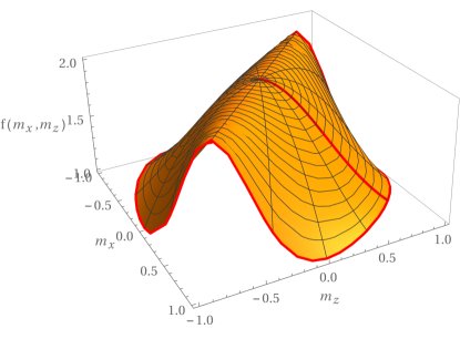
Figure 5: Plot of the function $f(m_{x},m_{z})$ (21) for $\mathbf{s}_{(i)}=\hat{\mathbf{e}}_{x}$. The red radial path drawn over the manifold is the profile of the one-dimensional function $m_{x}\mapsto f(m_{x},m_{x})$.

Consequently the probabilities for the particle to take either path after passing through the BS are given by

$$w_{\pm}=\frac{1\pm s_{(1)z}}{2}=\frac{1}{2}(1\pm s_{(i)z}\cos\omega\mp s_{(i)x}\sin\omega).$$ (26)

However, varying $\omega$ does not change the main result: if we still consider a preparation state $\mathbf{s}_{(i)}=s_{x}\hat{\mathbf{e}}_{x}$, we get the following expression for the sum $\mathcal{P}^{2}+\mathcal{V}^{2}$

$$\mathcal{P}^{2}+\mathcal{V}^{2}=s_{x}^{2}\left(\sin^{2}\omega+\frac{\frac{1}{4}\left(\sin 2\Theta\cos 2\omega\sin\xi+\sin 2\omega\cos 2\Theta+\sin 2\omega\sin^{2}\Theta\cos^{2}\xi\right)^{2}+\sin^{2}\Theta\cos^{2}\xi}{\left[1-\frac{s_{x}}{2}\left(\sin 2\Theta\cos 2\omega\sin\xi+\sin 2\omega\cos 2\Theta+\sin 2\omega\sin^{2}\Theta\cos^{2}\xi\right)\right]^{2}}\right),$$ (27)

which still spans all the range of values $0\leq\mathcal{P}^{2}+\mathcal{V}^{2}\leq 2$ and is saturated by the pure state $s_{x}=1$. Similarly, one can relax the condition $\mathbf{s}_{(i)}=s_{x}\hat{\mathbf{e}}_{x}$ to an arbitrary Bloch vector without any substantial difference.

The most immediate physical visualization of the generalized interferometer is a qubit undergoing a sequence of three precessions about the two axes $\hat{\mathbf{e}}_{y}$ and $\hat{\mathbf{m}}$, where the third rotation is the inverse of the first. It can be realized by applying sequentially three magnetic fields to a $1/2$-spin with a non-null magnetic moment. If one chooses the observable of interest to be the projection along the direction $\hat{\mathbf{e}}_{z}$, then the setup can be thought of as a binary interferometer: the two eigenvalues $\pm 1/2$ correspond to the two “paths”.

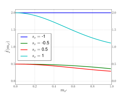
Figure 6: The function $\tilde{f}(s_{x},m_{x^{\prime}})$, Eq. (23), plotted for different initial states $\mathbf{s}_{(i)}=s_{x}\hat{\mathbf{e}}_{x}$, shows how the interferometric duality’s upper bound is $2$, corresponding to $\mathcal{P}=\mathcal{V}=1$. The plot with $s_{x}=1$ corresponds to the red radial profile shown in Fig. 5.

In our generalized scheme the unitary $U$ is no longer a phase-shifter. Indeed, a generic $2\times 2$ unitary matrix can be factorized as

$$U=e^{i\varphi}\begin{pmatrix}e^{i\psi}&0\\ 0&e^{-i\psi}\end{pmatrix}\begin{pmatrix}\cos\chi&\sin\chi\\ -\sin\chi&\cos\chi\end{pmatrix}\begin{pmatrix}e^{i\Delta}&0\\ 0&e^{-i\Delta}\\ \end{pmatrix},$$ (28)

which means that, in our coordinates representation, it can be thought of as a composition of two phase shifts and a beam splitter (up to an overall phase factor $e^{i\varphi}$) according to the sequence

$$U=e^{i\psi\sigma_{z}}e^{i\chi\sigma_{y}}e^{i\Delta\sigma_{z}}.$$ (29)

Therefore the action of the optical operation represented by $U_{2}$ consists of a first differential phase shift of an amount $2\Delta$, followed by a beam splitter and then by another $2\psi$-phase shift. Nevertheless our optical setup keeps the structure of an interferometer since, as we have already pointed out, the initial and final unitaries still act as two beam splitters.

VI Conclusions

In this work we have analysed a linear optical setup which can be considered as a natural generalization of the standard Mach-Zender interferometer. This setup is formally implemented by three consecutive unitary operators: the first and the last one still represent two beam splitters, while the middle one is a generic unitary.

We have derived a new duality relation involving two quantities, the fringe visibility $\mathcal{V}$ and the predictability $\mathcal{P}$, which are widely used to characterize the sharpness of the interference pattern and the amount of available information about the which-path observable, respectively. This duality relation is an inequality of the form

$$\mathcal{P}^{2}+\mathcal{V}^{2}\leq L_{U},$$

but its upper bound $L_{U}=\max_{\rho_{(i)}}\{\mathcal{P}^{2}+\mathcal{V}^{2}\}$, unlike the Mach-Zender interferometer, can assume values between $1$ and $2$. We have also shown how this upper bound depends on the parameters of the generalized interferometer.

Some considerations are in order. On the one hand the inequality (1) is commonly interpreted as the expression of a genuinely quantum property, the wave-particle duality. Nevertheless it is known that classical macroscopic objects can show a very similar behaviour Bush (2010). On the other hand our findings indicate that the trade-off between the so called “particle-like” and “wave-like” behaviour is in fact the property of a specific kind of interferometer and that it disappears when considering more general schemes of two-way interferometers. We think that the framework introduced in section III, where the parameters of the central unitary are not fixed, can be adapted to different kinds of situations and may inspire the study of new types of interferometric setups and experiments. In particular, Eq. (29) indicates that the abstract unitary $U$ can be operationally implemented as a sequence of optical transformations made of beam-splitters and phase-shifters.

Finally we believe that our work poses an interesting issue which is worth to be further investigated both theoretically and experimentally. If we accept that wave-particle duality is a distinctive feature of quantum mechanics (according Feynman the only “mystery” of quantum mechanics) then our inequality seems to suggest that, in the best case, duality does not imply incompatibility as in the common interpretation of Eq. (1). Another possible consequence is that all these relations are not actually able to capture the “mystery”, namely that quantities like $\mathcal{P}$ and $\mathcal{V}$ are not valid witnesses of the dual nature of quantum systems.

References

- Bohr (1928) N. Bohr, Nature 121, 580 (1928).
- Wootters and Zurek (1979) W. K. Wootters and W. H. Zurek, Phys. Rev. D 19, 473 (1979).
- Bartell (1980) L. S. Bartell, Phys. Rev. D 21, 1698 (1980).
- Greenberger and Yasin (1988) D. M. Greenberger and A. Yasin, Physics Letters A 128, 391 (1988).
- Englert (1996) B.-G. Englert, Phys. Rev. Lett. 77, 2154 (1996).
- Jaeger et al. (1993) G. Jaeger, M. A. Horne, and A. Shimony, Phys. Rev. A 48, 1023 (1993).
- Jaeger et al. (1995) G. Jaeger, A. Shimony, and L. Vaidman, Phys. Rev. A 51, 54 (1995).
- Englert and Bergou (2000) B.-G. Englert and J. A. Bergou, Optics Communications 179, 337 (2000).
- Martinez-Linares and Harmin (2004) J. Martinez-Linares and D. A. Harmin, Phys. Rev. A 69, 062109 (2004).
- Luis (2004) A. Luis, Phys. Rev. A 70, 062107 (2004).
- Englert et al. (2008) B.-G. Englert, D. Kaszlikowski, L. C. Kwek, and W. H. Chee, Int. J. Quantum Inform. 06, 129 (2008).
- Erez et al. (2009) N. Erez, D. Jacobs, and G. Kurizki, J. Phys. B: At. Mol. Opt. Phys. 42, 114006 (2009).
- Liu et al. (2009) N.-L. Liu, L. Li, S. Yu, and Z.-B. Chen, Phys. Rev. A 79, 052108 (2009).
- Li et al. (2012) L. Li, N.-L. Liu, and S. Yu, Phys. Rev. A 85, 054101 (2012).
- Coles et al. (2014) P. J. Coles, J. Kaniewski, and S. Wehner, Nat Commun 5, 5814 (2014).
- Jia et al. (2014) A.-A. Jia, J.-H. Huang, T.-C. Zhang, and S.-Y. Zhu, Phys. Rev. A 89, 042103 (2014).
- Bera et al. (2015) M. N. Bera, T. Qureshi, M. A. Siddiqui, and A. K. Pati, Phys. Rev. A 92, 012118 (2015).
- Rauch and Summhammer (1984) H. Rauch and J. Summhammer, Physics Letters A 104, 44 (1984).
- Summhammer et al. (1987) J. Summhammer, H. Rauch, and D. Tuppinger, Phys. Rev. A 36, 4447 (1987).
- Liu et al. (2012) H.-Y. Liu, J.-H. Huang, J.-R. Gao, M. S. Zubairy, and S.-Y. Zhu, Phys. Rev. A 85, 022106 (2012).
- Tang et al. (2013) J.-S. Tang, Y.-L. Li, C.-F. Li, and G.-C. Guo, Phys. Rev. A 88, 014103 (2013).
- Yan et al. (2015) H. Yan, K. Liao, Z. Deng, J. He, Z.-Y. Xue, Z.-M. Zhang, and S.-L. Zhu, Phys. Rev. A 91, 042132 (2015).
- Heuer et al. (2015) A. Heuer, G. Pieplow, and R. Menzel, Phys. Rev. A 92, 013803 (2015).
- Jacques et al. (2007) V. Jacques, E. Wu, F. Grosshans, F. Treussart, P. Grangier, A. Aspect, and J.-F. Roch, Science 315, 966 (2007).
- Jacques et al. (2008) V. Jacques, E. Wu, F. Grosshans, F. Treussart, P. Grangier, A. Aspect, and J.-F. Roch, Phys. Rev. Lett. 100, 220402 (2008).
- Manning et al. (2015) A. G. Manning, R. I. Khakimov, R. G. Dall, and A. G. Truscott, Nat Phys 11, 539 (2015).
- Arndt et al. (1999) M. Arndt, O. Nairz, J. Vos-Andreae, C. Keller, G. van der Zouw, and A. Zeilinger, Nature 401, 680 (1999).
- Couder et al. (2005) Y. Couder, S. Protière, E. Fort, and A. Boudaoud, Nature 437, 208 (2005).
- Couder and Fort (2006) Y. Couder and E. Fort, Phys. Rev. Lett. 97, 154101 (2006).
- Bush (2010) J. W. M. Bush, PNAS 107, 17455 (2010).