A Parallel Orbital-updating Based Optimization Method for Electronic Structure Calculations

Abstract

In this paper, we propose a parallel optimization method for electronic structure calculations based on a single orbital-updating approximation. It is shown by our numerical experiments that the method is efficient and reliable for atomic and molecular systems of large scale over supercomputers.

1 Introduction

Kohn-Sham equations are nonlinear eigenvalue problems and typical models used in electronic structure calculations. Due to the nonlinearity and requirement of a cluster of eigenpairs, it is desired and significant to design efficient and in particular supercomputer friendly numerical methods for solving Kohn-Sham equations. Most recently, a so-called parallel orbital-updating algorithm has been proposed in [2] to Kohn-Sham equations and been demonstrated to be a quite potential approach for electronic structure calculations over supercomputers.

Note that in the context of solving nonlinear eigenvalue problems, the self consistent field (SCF) iteration is most widely used. However, the convergence of SCF is not guaranteed, especially for large scale systems with small band gaps, its performance is unpredictable [21]. As a result, optimization algorithms have been developed for the Kohn-Sham direct energy minimization models, which are different from solving the nonlinear eigenvalue models, including trust region type methods [4, 5, 11, 15], Newton-type methods [3, 6], conjugate gradient methods [8, 13, 18], and gradient-type methods [17, 19, 21] (see, also, [10, 20] and references cited therein). We particularly mention that the gradient type method proposed in [21] constructs new trail points along the gradient on the Stiefel manifold and has been shown to be efficient and robust. However, to develop a parallel optimization algorithm is still significant and challenging for electronic structure calculations, especially for systems of large scale over supercomputers.

We observe that optimization algorithms often have better convergence properties: as long as the ground state is not orthogonal to the starting point, the ground state is reachable from any starting point by following a path of decreasing energy [14]. In this paper, we shall apply a similar idea of [2] to direct energy minimization models and propose a parallel approach to electronic structure calculations based on a single orbital-updating approximation.

We understand that the parallel orbital-updating algorithm proposed in [2] reduces the large scale eigenvalue problem to the solution of some independent source problems and some eigenvalue problem of small systems, and the source problems are independent each other and can be calculated in parallel intrinsically. While in this paper, instead of solving the large global energy minimization problem, we simply minimize the total energy functional along each orbital direction independently and then orthonormalize the orbital minimizers obtained, which is a two-level parallelism similar to [2]. We should mention that in practice, it is not easy and unnecessary to find the minimum for each orbital in each iteration. Instead, we solve the $N$ optimization subproblems approximately or inexactly.

The rest of this paper is organized as follows: in Section 2, we provide a brief introduction to the Kohn-Sham density functional theory (DFT) model and its associated Stiefel manifold. We then propose our parallel orbital-updating based optimization algorithms for electronic structure calculations in Section 3. We present numerical results in Section 4 to show the accuracy and efficiency of our algorithms. Finally, we give some concluding remarks in Section 5.

2 Preliminaries

2.1 Kohn-Sham DFT model

Let $\mathcal{U}=(u_{1},\dots,u_{N})$, with $u_{i}\in H^{1}(\mathbb{R}^{3})$, the Kohn-Sham DFT model solves the following constrained optimization problem

(1) $$\begin{split}&\inf\ \ \ E(\mathcal{U})\\ s.t.\ \ &\int_{\mathbb{R}^{3}}u_{i}(r)u_{j}(r)dr=\delta_{ij},\ \ 1\leq i,j\leq N,\end{split}$$

where the Kohn-Sham total energy $E(\mathcal{U})$ is defined as

(2) $$E(\mathcal{U}) = \frac{1}{2}\int_{\mathbb{R}^{3}}\sum_{i=1}^{N}|\nabla u_{i}(r)|^{2}dr+\frac{1}{2}\int_{\mathbb{R}^{3}}\int_{\mathbb{R}^{3}}\frac{\rho(r)\rho(r^{\prime})}{|r-r^{\prime}|}drdr^{\prime}$$

$$+\int_{\mathbb{R}^{3}}\sum_{i=1}^{N}u_{i}(r)V_{ext}(r)u_{i}(r)dr+\int_{\mathbb{R}^{3}}\varepsilon_{xc}(\rho(r))\rho(r)dr.$$

Here $\rho(r)=\sum\limits_{i=1}^{N}|u_{i}(r)|^{2}$ is the electronic density, $V_{ext}(r)$ is the external potential generated by the nuclei: for full potential calculations, $V_{ext}(r)=-\sum\limits_{I=1}^{M}\frac{Z_{I}}{|r-R_{I}|}$, $Z_{I}$ and $R_{I}$ are the nuclei charge and position of the $I$-th nuclei respectively; while for pseudo potential approximations, $V_{ext}(r)=\sum\limits_{I=1}^{M}V^{I}_{loc}(r)+V^{I}_{nloc}(r)$, $V^{I}_{loc}(r)$ is the local part of the pseudo potential for nuclei $I$, $V^{I}_{nloc}(r)$ is the nonlocal part, which usually has the following form

$$V^{I}_{nloc}u(r)=\sum_{l}\int_{\mathbb{R}^{3}}\xi_{l}^{I}(r^{\prime})u(r^{\prime})dr^{\prime}\xi_{l}^{I}(r),$$

with $\xi_{l}^{I}\in L^{2}(\mathbb{R}^{3})$ [7]. The $\varepsilon_{xc}(\rho(r))$ in the forth term is the exchange-correlation functional, describing the many-body effects of exchange and correlation [7], which is not known explicitly, and some approximation (such as LDA, GGA) has to be used. The functions $\{u_{i},i=1,\dots,u_{N}\}$ are call Kohn-Sham orbitals.

Denote $E_{u_{i}}$ the derivative of $E(\mathcal{U})$ to the $i$-th orbital, it is easy to see that

$$E_{u_{i}}=H(\rho)u_{i},$$

where

$$H(\rho)=-\frac{1}{2}\Delta+V_{ext}+\int_{\mathbb{R}^{3}}\frac{\rho(r^{\prime})}{|r-r^{\prime}|}dr^{\prime}+v_{xc}(\rho),$$

here $v_{xc}(\rho)=\frac{\text{d}(\rho\varepsilon_{xc}(\rho))}{\text{d}\rho}$ is the exchange correlation potential, $H(\rho)$ is the Kohn-Sham Hamiltonian operator.

2.2 Stiefel manifold and gradient

The feasible set of the constraint problem (1) is a Stiefel manifold, which is defined as

$$\mathcal{M}_{V}^{N}=\{\mathcal{U}=(u_{i})_{i=1}^{N}|u_{i}\in V,\langle\mathcal{U}^{T}\mathcal{U}\rangle=I_{N}\},$$

where $V=H^{1}(\mathbb{R}^{3})$, and for $\Psi=(\psi_{1},\dots,\psi_{N})\in V^{N}$, $\Phi=(\phi_{1},\dots,\phi_{N})\in V^{N}$, the inner product matrix is defined as $\langle\Psi^{T}\Phi\rangle:=(\langle\psi_{i},\phi_{j}\rangle)_{ij=1}^{N}\in\mathbb{R}^{N\times N}$, $\langle\psi_{i},\phi_{j}\rangle=\int_{\mathbb{R}^{3}}\psi_{i}(r)\phi_{j}(r)dr$ is the usual $L_{2}$ inner product. By computing the derivative of the constraint condition

$$\langle\mathcal{U}^{T}\mathcal{U}\rangle=I_{N},$$

we get the tangent space of $\mathcal{M}_{V}^{N}$ at $\mathcal{U}$

$$\mathcal{T}_{\mathcal{U}}\mathcal{M}_{V}^{N}=\{\mathcal{B}\in V^{N}:\langle\mathcal{U}^{T}\mathcal{B}\rangle=-\langle\mathcal{B}^{T}\mathcal{U}\rangle\in\mathbb{R}^{N\times N}\}.$$

We verify from (2) that $E(\mathcal{U})=E(\mathcal{U}P)$ for any $N\times N$ orthogonal matrix $P$. To get rid of the non uniqueness, we consider the problem on the Grassmann manifold, which is the quotient of the Stiefel manifold and defined as

$$\mathcal{G}_{V}^{N}=\mathcal{M}_{V}^{N}/\sim,$$

here $\mathcal{U}\sim\tilde{\mathcal{U}}$ if there is an orthogonal matrix $P$ such that $\tilde{\mathcal{U}}=\mathcal{U}P$, we use $[\mathcal{U}]$ to denote the equivalence class. The tangent space of the Grassmann manifold $\mathcal{G}_{V}^{N}$ at $[\mathcal{U}]$ is [12]

$$\mathcal{T}_{[\mathcal{U}]}\mathcal{G}_{V}^{N}=\{\mathcal{F}\in V^{N}:\langle\mathcal{F}^{T}\mathcal{U}\rangle=0\in\mathbb{R}^{N\times N}\}.$$

By the first order necessary condition, we see that the derivative $E^{\prime}(\mathcal{U})$ of the energy $E(\mathcal{U})$ at the minimizer $[\mathcal{U}]\in\mathcal{G}_{V}^{N}$ satisfies [12]

$$\text{tr}\langle(E^{\prime}(\mathcal{U}))^{T}\delta\mathcal{U}\rangle=\text{tr}\langle(H(\rho)\mathcal{U})^{T}\delta\mathcal{U}\rangle=0,\ \ \ \forall\ \delta\mathcal{U}\in\mathcal{T}_{[\mathcal{U}]}\mathcal{G}_{V}^{N},$$

i.e. the derivative $E^{\prime}(\mathcal{U})$ vanishes on the tangent space $\mathcal{T}_{[\mathcal{U}]}\mathcal{G}_{V}^{N}$ of the Grassmann manifold, we then get the gradient $\nabla E(\mathcal{U})$ of the energy on the Stiefel manifold

(3) $$\nabla E(\mathcal{U})=H(\rho)\mathcal{U}-\mathcal{U}\Sigma=0,$$

where $\Sigma=\langle(H(\rho)\mathcal{U})^{T}\mathcal{U}\rangle$ is symmetric since the Hamiltonian $H(\rho)$ is a symmetric operator. Suppose orthogonal matrix $P$ diagonalize $\Sigma$, i.e. $P^{T}\Sigma P=\Lambda$, where $\Lambda$ is a diagonal matrix, let $\mathcal{U}=\mathcal{U}P$, substitute into (3), notice that $\rho=\sum\limits_{i=1}^{N}|u_{i}|^{2}$ is invariant under the orthogonal transformation, we get the well known Kohn-Sham equation

(4) $$H(\rho)\mathcal{U}=\mathcal{U}\Lambda,\ \ s.t.\ \ \langle\mathcal{U}^{T}\mathcal{U}\rangle=I_{N}.$$

2.3 Discretization

The continuous Kohn-Sham DFT model can be discretized by either real space approaches including finite difference, finite element ect., or by planewave basis. We focus on the real space discretization in this paper. For simplicity, we still use the notations as in the previous part for the discretized problem. Note that this does not affect the algorithm we propose in this paper.

As will be shown in section 3, since the mesh and hence the finite dimensional space is changing, we denote the discretized finite dimensional space by $V^{(n)}$ in outer iteration $n$. For the inner loop, the solution $\mathcal{W}^{(l)}$ is in the space $V^{(n)}$.

3 Parallel orbital-updating based optimization algorithm

3.1 General framework

Motivated by [2], we propose a parallel orbital-updating based optimization algorithm, whose general framework is shown as Algorithm 1.

Algorithm 1

1:  Given initial space $V^{(0)}$, initial data $\mathcal{U}^{(0)},\ s.t.\ \langle(\mathcal{U}^{(0)})^{T}\mathcal{U}^{(0)}\rangle=I_{N}$, let $n=0$;

2:  Apply an adaptive approach to $\mathcal{U}^{(n)}$ and get $V^{(n+1)}$;

3:  $\mathcal{W}^{(0)}=\mathcal{U}^{(n)}$, $l=0$;

4:  For $i=1,\dots,N$, apply an optimization approach to get $\widetilde{w}_{i}^{(l+1)}$ in parallel, such that

$$E(\mathcal{W}^{(l)}_{i}\diamond{\tilde{w}}^{(l+1)}_{i})<E(\mathcal{W}^{(l)}),$$

where $\mathcal{W}^{(l)}_{i}\diamond v=(w_{1}^{(l)},\dots,w_{i-1}^{(l)},v,w_{i+1}^{(l)},\dots,w_{N}^{(l)})$;

5:  $\mathcal{W}^{(l+1)}=\text{Orth}(\widetilde{\mathcal{W}}^{(l+1)}),\ l=l+1$;

6:  Convergence check for the inner iteration: if not converged, goto step 4;

7:  $\mathcal{U}^{(n+1)}=\mathcal{W}^{(l)}$, $n=n+1$;

8:  Convergence check for the outer iteration: if not converged, goto step 2; else, stop.

Fig. 1: Flowchart for Algorithm 1

We see from Algorithm 1 that there are two level iterations here: the outer iteration is for mesh refinement, and the inner loop for optimization along each orbital in parallel. Various optimization approaches can be applied to solve the optimization subproblems, such as the Newton’s method, the steepest descent method, and the conjugate gradient method, etc.. In this paper, we focus on the first order algorithms. In our experiments, the choices of search direction and step size shown are based on the steepest descent method.

3.2 Search direction and step size

We see that the search direction and step size are the most important parts of an optimization algorithm, which are critical to the speed of convergence. Here, we choose the approximated gradient of the energy function on the Stiefel manifold as the search direction, and step size is determined by the Barzilai-Borwein (BB) formula [1].

Note that two gradient type optimization algorithms are proposed in [21]. One of them is OptM-QR that calculates $\widetilde{\mathcal{W}}=\mathcal{W}-\tau\nabla E(\mathcal{W})$, and then orthogonalize $\widetilde{\mathcal{W}}$ by using the QR factorization, i.e. $\mathcal{W}^{\text{new}}=\text{qr}(\mathcal{W})$.

We see that if the orbitals $\{w_{i}\}_{i=1}^{N}$ are the eigenfuctions of the Hamiltonian $H(\rho_{\mathcal{W}})$, the matrix $\Sigma:=\langle(E^{\prime}(\mathcal{W}))^{T}\mathcal{W}\rangle$ will be diagonal. Based on this observation, we choose the diagonal element $\sigma_{ii}$ of $\Sigma$ to approximate the matrix, that is we choose $z_{i}^{(l)}=H(\mathcal{W}^{(l)})w_{i}^{(l)}-\sigma_{ii}^{(l)}w_{i}^{(l)}$ as our search direction, where $\sigma_{ii}^{(l)}=\langle H(\mathcal{W}^{(l)})w_{i}^{(l)},w_{i}^{(l)}\rangle$. Then we can calculate the search direction for each orbital in parallel.

In step $l$, we choose the following BB step size (we use the same step size for all orbitals):

$$\tau_{i}^{l,1}=\frac{\text{tr}\langle(\mathcal{S}^{(l-1)})^{T}\mathcal{S}^{(l-1)}\rangle}{\text{tr}|\langle(\mathcal{S}^{(l-1)})^{T}\mathcal{Y}^{(l-1)}\rangle|}\ \ \text{or}\ \ \tau_{i}^{l,2}=\frac{\text{tr}|\langle(\mathcal{S}^{(l-1)})^{T}\mathcal{Y}^{(l-1)}\rangle|}{\text{tr}\langle(\mathcal{Y}^{(l-1)})^{T}\mathcal{Y}^{(l-1)}\rangle},$$

where $\mathcal{S}^{(l-1)}=\mathcal{W}^{(l)}-\mathcal{W}^{(l-1)}$, $\mathcal{Y}^{(l-1)}=\mathcal{Z}^{(l)}-\mathcal{Z}^{(l-1)}$. The calculations of the diagonal elements above can be done in parallel for each orbital.

In order to guarantee convergence, we perform back tracing for the step size. Let $C^{(0)}=E(\mathcal{W}^{(0)})$, $Q^{(l+1)}=\eta Q^{(l)}+1$, $Q^{(0)}=1$. Then $\mathcal{W}^{(l+1)}=\mathcal{W}(\tau^{(l)})$, where the $\mathcal{W}(\tau^{(l)})$ is the new point we get in Algorithm 1 in step 4-5 ($\tau^{(l)}_{i}=\tau^{(l)}$), and $\tau^{(l)}=\tau_{i}^{l,1}\delta^{s}$ or $\tau^{(l)}=\tau_{i}^{l,2}\delta^{s}$, $s$ is smallest nonnegative integer satisfying

(5) $$E(\mathcal{W}(\tau^{(l)}))\leq C^{(l)}-\rho_{1}\tau^{(l)}\|\mathcal{Z}^{(l)}\|_{F}^{2},$$

where $C^{(l+1)}=(\eta Q^{(l)}C^{(l)}+E(\mathcal{W}^{(l+1)}))/Q^{(l+1)}$, $\eta$, $\delta$ and $\rho_{1}$ are constant factors, we choose $\rho_{1}=1\times 10^{-4}$, $\delta=0.1$ and $\eta=0.85$ in our numerical experiments.

Algorithm 1 with the above implementation details is named as Algorithm 2.

Algorithm 2

1:  Given initial space $V^{(0)}$, initial data $\mathcal{U}^{(0)},\ s.t.\ \langle(\mathcal{U}^{(0)})^{T}\mathcal{U}^{(0)}\rangle=I_{N}$, let $n=0$;

2:  Apply an adaptive approach to $\mathcal{U}^{(n)}$ and get $V^{(n+1)}$;

3:  $\mathcal{W}^{(0)}=\mathcal{U}^{(n)}$, $l=0$;

4:  Calculate the search directions $\{z_{i}^{(l)}\}_{i=1}^{N}$ in parallel;

5:  Calculate the step size $\tau_{i}^{l}=\tau_{i}^{l,1}\delta^{s}$ or $\tau_{i}^{l}=\tau_{i}^{l,2}\delta^{s}$, where $s$ is the smallest nonnegative integer such that (5) is satisfied;

6:  $\mathcal{W}^{(l+1)}=\text{Orth}(\widetilde{\mathcal{W}}^{(l+1)}),\ l=l+1$;

7:  Convergence check for the inner iteration: if not converged, goto step 4;

8:  $\mathcal{U}^{(n+1)}=\mathcal{W}^{(l)}$, $n=n+1$;

9:  Convergence check for the outer iteration: if not converged, goto step 2; else, stop.

As in Proposition 3.2 in [21], if we use the full $\Sigma$ for all the orbitals, the resulting $\widetilde{\mathcal{W}}$ is full rank and $\langle\widetilde{\mathcal{W}}^{T}\widetilde{\mathcal{W}}\rangle$ is well conditioned, which makes it easy to perform QR factorization based on Cholesky factorization. While for the algorithm proposed here, we do not have the theoretical result to ensure this property. However, this is not a problem to perform the QR factorization numerically (if we use the subspace diagonalization technique introduced in the next subsection), and we observe from Figure 2 that the matrix $\langle\widetilde{\mathcal{W}}^{T}\widetilde{\mathcal{W}}\rangle$ is diagonal dominated and very close to identity matrix.

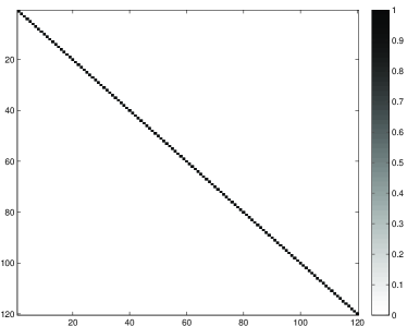
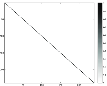
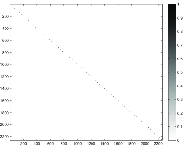
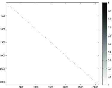
Fig. 2: The matrix $\langle\widetilde{\mathcal{W}}^{T}\widetilde{\mathcal{W}}\rangle$ for $C_{60}$ and $C_{120}$, $C_{1015}H_{460}$ and  $C_{1419}H_{556}$ by Algorithm 3, at iteration step 101, with $n_{diag}$ = 100, $n_{orthg}$ = 2.

3.3 Modifications

As the iteration goes on, the matrix $\Sigma:=\langle(E^{\prime}(\mathcal{W}))^{T}\mathcal{W}\rangle$ deviates from diagonal matrix gradually, the error to approximate the gradient by choosing the diagonal elements of $\Sigma$ becomes larger and larger. Therefore, we perform subspace diagonalization for the Hamiltonian in the space spanned by current orbitals every $n_{diag}$ (a parameter) steps. Specifically, suppose orthogonal matrix $P\in\mathbb{R}^{N\times N}$ diagonalize $\Sigma$, i.e. $P^{T}\Sigma P=\Gamma$ ($\Gamma$ is diagonal), let $\mathcal{W}^{\text{new}}=\mathcal{W}P$. Then if $\langle\mathcal{W}^{T}\mathcal{W}\rangle=I_{N}$, we have $\langle(\mathcal{W}^{\text{new}})^{T}\mathcal{W}^{\text{new}}\rangle=P^{T}\langle(\mathcal{W}^{T}\mathcal{W})\rangle P=I_{N}$, $\rho(\mathcal{W}^{\text{new}})=\rho(\mathcal{W})$. Since $H(\mathcal{W})$ is determined by $\rho(\mathcal{W})$, we have $H(\mathcal{W}^{\text{new}})=H(\mathcal{W})$, then $\Sigma^{\text{new}}:=\langle(H(\mathcal{W}^{\text{new}})\mathcal{W}^{\text{new}})^{T}\mathcal{W}^{\text{new}}\rangle$ is diagonal.

We see from Algorithm 2 that the main part of calculations we cannot carry out in parallel for each orbital are the orthogonalization of orbitals in step 6. To decrease this part of time, we perform orthogonalization every $n_{org}$ steps. That is, we do not orthogonalize the orbitals every iteration. As a result, we calculate the total energy and perform back tracing for the step size every $n_{org}$ steps. Such a modified algorithm is stated as Algorithm 3:

Algorithm 3

1:  Given initial space $V^{(0)}$, initial data $\mathcal{U}^{(0)},\ s.t.\ \langle(\mathcal{U}^{(0)})^{T}\mathcal{U}^{(0)}\rangle=I_{N}$, $n_{orthg}$ and $n_{diag}$, let $n=0$;

2:  Apply an adaptive approach to $\mathcal{U}^{(n)}$ and get $V^{(n+1)}$;

3:  $\mathcal{W}^{(0)}=\mathcal{U}^{(n)}$, $l=0$;

4:  Calculate the search directions $\{z_{i}^{(l)}\}_{i=1}^{N}$ in parallel;

5:  if (mod(l, $n_{org}$) $\neq$ 0) then

6:     Calculate the step size $\tau_{i}^{l}=\tau_{i}^{l,1}$ or $\tau_{i}^{l}=\tau_{i}^{l,2}$, let $w_{i}^{(l+1)}=w_{i}^{(l)}-\tau_{i}^{(l)}z_{i}^{(l)}$, $l=l+1$;

7:  else

8:     Calculate the step size $\tau_{i}^{l}=\tau_{i}^{l,1}\delta^{s}$ or $\tau_{i}^{l}=\tau_{i}^{l,2}\delta^{s}$, where $s$ is the smallest nonnegative integer such that (5) is satisfied;

9:     $\mathcal{W}^{(l+1)}=\text{Orth}(\widetilde{\mathcal{W}}^{(l+1)}),\ l=l+1$;

10:     If $mod(l,n_{diag})=0$, let $\mathcal{W}^{(l+1)}=\mathcal{W}^{(l+1)}P^{(l+1)}$, where $P^{(l+1)}$ is the rotation matrix introduced in the previous subsection;

11:  end if

12:  Convergence check for the inner iteration: if not converged, goto step 4;

13:  $\mathcal{U}^{(n+1)}=\mathcal{W}^{(l)}$, $n=n+1$;

14:  Convergence check for the outer iteration: if not converged, goto step 2; else, stop.

4 Numerical experiments

Our numerical experiments are carried out on the software package OCTOPUS(version 4.0.1), a real space ab initio computing platform. We choose local density approximation (LDA) to approximate $v_{xc}(\rho)$ [9] in our numerical experiments. The initial guess of the orbitals is generated by linear combination of the atomic orbits (LCAO) method, and the Troullier-Martins norm conserving pseudopotential [16] is used in our computation. We use Algorithm 3 for all the tests, and the current results are without mesh refinement.

Our examples include several typical molecular systems: benzene ($C_{6}H_{6}$), aspirin ($C_{9}H_{8}O_{4})$, fullerene ($C_{60}$), alanine chain $(C_{33}H_{11}O_{11}N_{11})$, carbon nano-tube ($C_{120}$), biological ligase 2JMO $(C_{178}H_{283}O_{50}N_{57}S)$, protein fasciculin2 $(C_{276}H_{442}O_{90}N_{88}S_{10})$, carbon cluster $C_{1015}H_{460}$ and $C_{1419}H_{556}$.

4.1 Reliability

We first test the reliability of out algorithm. The results are shown in Table 1. The Opt-Z3W is the OptM-QR algorithm in [21], Opt-Par is the parallel orbital-updating based optimization algorithm proposed in this paper. The column ’energy’ is the Kohn-Sham total energy (in atomic units), ’iter’ denotes the total number of iterations, and ’resi’ denotes the norm of the residual $\|\nabla E(\mathcal{U})\|=\sqrt{\text{tr}\langle\nabla E(\mathcal{U})^{T}\nabla E(\mathcal{U})\rangle}$. We use ’cores’ to denote the number of CPU cores used in that calculation, and it is chosen as $2^{s}$, where $s$ is the largest integer that makes the number of elements on each processor not smaller than the value recommended by Octopus.

We choose $n_{diag}=100$, $n_{org}=1$. Since the mesh refinement is not implemented, we use $\|\nabla E(\mathcal{U})\|<10^{-6}$ as the convergence criterion for the inner iteration. And since it is difficult to converge to this criterion for large systems, we choose a looser criterion, that is: the average of absolute value of each element of the matrix $\nabla E(\mathcal{U})$ is less than $5\times 10^{-9}$. So, for 2JMO, FAS2, $C_{1015}H_{460}$ and $C_{1419}H_{556}$, the practical convergence criteria are $4.06\times 10^{-5},6.48\times 10^{-5},7.62\times 10^{-5}\ \mbox{and}\ 1.01\times 10^{-4}$.

Table 1: The results using $\|\nabla E\|_{F}$ as convergence criteria, $n_{diag}=100$, $n_{org}=1$.

algorithm	energy	iter	resi	total-time(s)
benzene($C_{6}H_{6})\ \ \ N_{g}=102705\ \ \ N=15\ \ \ cores=8$
Opt-Z3W	-3.74246025E+01	164	7.49E-07	6.63
Opt-Par	-3.74246025E+01	173	7.95E-07	7.58
aspirin($C_{9}H_{8}O_{4})\ \ \ N_{g}=133828\ \ \ N=34\ \ \ cores=16$
Opt-Z3W	-1.20214764E+02	153	9.89E-07	15.67
Opt-Par	-1.20214764E+02	134	9.55E-07	17.33
$C_{60}\ \ \ N_{g}=191805\ \ \ N=120\ \ \ cores=16$
Opt-Z3W	-3.42875137E+02	222	9.02E-07	96.73
Opt-Par	-3.42875137E+02	230	9.43E-07	108.24
alanine chain$(C_{33}H_{11}O_{11}N_{11})\ \ \ N_{g}=293725\ \ \ N=132\ \ \ cores=32$
Opt-Z3W	-4.78562217E+02	1779	9.60E-07	1036.44
Opt-Par	-4.78562217E+02	1673	9.87E-07	1101.63
$C_{120}\ \ \ N_{g}=354093\ \ \ N=240\ \ \ cores=32$
Opt-Z3W	-6.84467048E+02	2392	9.64E-07	2560.63
Opt-Par	-6.84467048E+02	1848	9.42E-07	2274.45
2JMO$(C_{178}H_{283}O_{50}N_{57}S)\ \ \ N_{g}=1226485\ \ \ N=793\ \ \ cores=128$
Opt-Z3W	-2.56413551E+03	1502	4.03E-05	11998.30
Opt-Par	-2.56413551E+03	1846	4.05E-05	18201.79
FAS2$(C_{276}H_{442}O_{90}N_{88}S_{10})\ \ \ N_{g}=1903841\ \ \ N=1293\ \ \ cores=256$
Opt-Z3W	-4.26018875E+03	2050	6.46E-05	30152.76
Opt-Par	-4.26018881E+03	2094	6.48E-05	44952.46
$C_{1015}H_{460}\ \ \ N_{g}=1462257\ \ \ N=2260\ \ \ cores=256$
Opt-Z3W	-6.06369982E+03	137	3.08E-05	5331.19
Opt-Par	-6.06369982E+03	144	7.26E-05	6217.72
$C_{1419}H_{556}\ \ \ N_{g}=1828847\ \ \ N=3116\ \ \ cores=512$
Opt-Z3W	-8.43085432E+03	151	1.01E-04	9084.88
Opt-Par	-8.43085432E+03	138	5.49E-05	9453.76

We see from Table 1 that for all the systems, Opt-Par get the same convergence result as Opt-Z3W, which confirms the reliability of our algorithm.

We show the energy reduction $E(X^{(n)})-E_{min}$ for $C_{60}$ and 2JMO in Figure 3, where $E_{min}$ is a reliable minimum of the total energy. We can see that although there are some oscillations, the energy decreases gradually until convergence is reached.

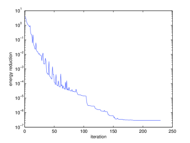
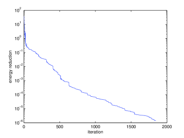
Fig. 3: Energy reduction for C60 and 2JMO.

4.2 Parallelism

In this subsection, we test the parallelism in orbital for our algorithm. Since the parallel in orbital is not implemented yet, we show the computation time in two parts: the first part is the total computation time (’total-time’), the second part is the time that can be done parallel in each orbital (’par-time’), ’percent’ is ’par-time’ divided by ’total-time’. Because it costs too much time to calculate the residual $\|\nabla E(\mathcal{U})\|$, and this part of calculations are not parallel in orbital, we use the relative change of total energy as our convergence criteria, that is: $\frac{df^{(l)}+df^{(l-1)}+df^{(l-2)}}{3}<10^{-13}$, where $df^{(l)}=\frac{|E(\mathcal{U}^{(l-1)})-E(\mathcal{U}^{(l)})|}{|E(\mathcal{U}^{(l-1)})|+1}$ (when we perform orthogonalization every $n_{org}$ steps, since we don’t calculate the energy step, we choose the average change of total energy of adjacent $n_{org}$ steps). We present the results under different parameters in the Tables 2 and 3.

Table 2: The results using convergence criteria $\frac{df^{(n)}+df^{(n-1)}+df^{(n-2)}}{3}<10^{-13}$, $n_{diag}=100$, $n_{org}=1$.

algorithm	energy	iter	resi	total-time(s)	par-time(s)	percent
benzene$\ \ \ N_{g}=102705\ \ \ N=15\ \ \ cores=8$
Opt-Z3W	-3.74246025E+01	165	7.93E-07	6.63	-	-
Opt-Par	-3.74246025E+01	168	2.87E-06	6.94	3.86	56%
aspirin$\ \ \ N_{g}=133828\ \ \ N=34\ \ \ cores=16$
Opt-Z3W	-1.20214764E+02	141	1.96E-06	15.67	-	-
Opt-Par	-1.20214764E+02	135	2.96E-06	14.52	8.23	57%
$C_{60}\ \ \ N_{g}=191805\ \ \ N=120\ \ \ cores=16$
Opt-Z3W	-3.42875137E+02	176	7.69E-06	99.66	-	-
Opt-Par	-3.42875137E+02	191	4.00E-05	80.64	54.44	68%
alanine chain$\ \ \ N_{g}=293725\ \ \ N=132\ \ \ cores=32$
Opt-Z3W	-4.78562217E+02	1538	1.73E-05	968.12	-	-
Opt-Par	-4.78562217E+02	1599	4.48E-05	942.87	576.32	61%
$C_{120}\ \ \ N_{g}=354093\ \ \ N=240\ \ \ cores=32$
Opt-Z3W	-6.84467048E+02	1390	1.80E-05	1588.33	-	-
Opt-Par	-6.84467048E+02	1435	4.53E-05	1403.23	1056.02	75%
2JMO$\ \ \ N_{g}=1226485\ \ \ N=793\ \ \ cores=128$
Opt-Z3W	-2.56413551E+03	1480	4.08E-05	14524.26	-	-
Opt-Par	-2.56413551E+03	1794	4.18E-05	13692.19	9564.53	70%
FAS2$\ \ \ N_{g}=1903841\ \ \ N=1293\ \ \ cores=256$
Opt-Z3W	-4.26018875E+03	2150	5.67E-05	43218.37	-	-
Opt-Par	-4.26018881E+03	2225	5.83E-05	37925.49	25147.62	66%
$C_{1015}H_{460}\ \ \ N_{g}=1462257\ \ \ N=2260\ \ \ cores=256$
Opt-Z3W	-6.06369982E+03	145	9.59E-06	5525.22	-	-
Opt-Par	-6.06369982E+03	157	1.41E-04	4873.35	3012.72	62%
$C_{1419}H_{556}\ \ \ N_{g}=1828847\ \ \ N=3116\ \ \ cores=512$
Opt-Z3W	-8.43085432E+03	165	5.05E-05	9926.59	-	-
Opt-Par	-8.43085432E+03	179	6.43E-05	9277.48	6223.67	67%

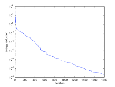
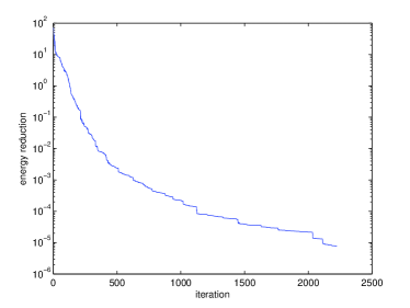
Fig. 4: Energy reduction for 2JMO and FAS2 (Correspond to Table 2).

Table 3: The results using convergence criteria $\frac{df^{(n)}+df^{(n-1)}+df^{(n-2)}}{3}<5\times 10^{-13}$, $n_{diag}=50$, $n_{org}=2$.

algorithm	energy	iter	resi	total-time(s)	par-time(s)	percent
benzene$\ \ \ N_{g}=102705\ \ \ N=15\ \ \ cores=8$
Opt-Z3W	-3.74246025E+01	142	9.76E-06	5.85	-	-
Opt-Par	-3.74246025E+01	153	4.72E-06	4.39	2.58	59%
aspirin$\ \ \ N_{g}=133828\ \ \ N=34\ \ \ cores=16$
Opt-Z3W	-1.20214764E+02	121	1.72E-05	12.68	-	-
Opt-Par	-1.20214764E+02	119	7.99E-06	9.61	5.55	58%
$C_{60}\ \ \ N_{g}=191805\ \ \ N=120\ \ \ cores=16$
Opt-Z3W	-3.42875137E+02	167	3.46E-05	73.18	-	-
Opt-Par	-3.42875137E+02	189	4.66E-05	84.50	39.37	72%
alanine chain$\ \ \ N_{g}=293725\ \ \ N=132\ \ \ cores=32$
Opt-Z3W	-4.78562217E+02	1017	2.90E-05	659.92	-	-
Opt-Par	-4.78562217E+02	1865	2.12E-05	778.51	559.43	72%
$C_{120}\ \ \ N_{g}=354093\ \ \ N=240\ \ \ cores=32$
Opt-Z3W	-6.84467046E+02	1200	5.05E-05	1396.19	-	-
Opt-Par	-6.84467048E+02	1965	1.88E-05	1346.37	1100.22	82%
2JMO$\ \ \ N_{g}=1226485\ \ \ N=793\ \ \ cores=128$
Opt-Z3W	-2.56413551E+03	1049	8.98E-05	9836.49	-	-
Opt-Par	-2.56413551E+03	1987	4.47E-05	9593.32	7180.12	75%
FAS2$\ \ \ N_{g}=1903841\ \ \ N=1293\ \ \ cores=256$
Opt-Z3W	-4.26018872E+03	1596	1.23E-04	31647.13	-	-
Opt-Par	-4.26018870E+03	2539	1.12E-04	26709.60	19401.66	73%
$C_{1015}H_{460}\ \ \ N_{g}=1462257\ \ \ N=2260\ \ \ cores=256$
Opt-Z3W	-6.06369982E+03	128	9.90E-05	4899.40	-	-
Opt-Par	-6.06369982E+03	139	3.23E-05	2615.67	1611.80	62%
$C_{1419}H_{556}\ \ \ N_{g}=1828847\ \ \ N=3116\ \ \ cores=512$
Opt-Z3W	-8.43085432E+03	150	1.02E-04	9135.69	-	-
Opt-Par	-8.43085432E+03	155	4.43E-05	5125.12	3143.89	61%

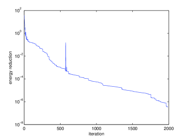
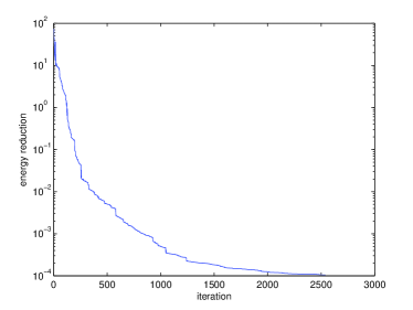
Fig. 5: Energy reduction for 2JMO and FAS2 (Correspond to Table 3).

We observe from Table 2 that: for larger system, the percentage of time that we can do parallel in orbital is larger than 65%, which is very attractive for large systems calculations. By choosing $n_{org}=2$, the parallel percentage is further increased, as shown in Table 3.

Figure 4 and 5 show the energy reduction for 2JMO and FAS2, which confirm the convergence of our algorithm. One may see that there are some oscillations in the energy reduction curve for 2JMO in Figure 5. This is due to we do not perform orthogonalization every step, the search direction may deviate from the energy decrease direction, and we do not perform back tracing for the step size in these steps. However, the oscillation steps are far form convergence, and there is no oscillation when the convergence is reached. Therefore, it does not affect the computational results.

5 Concluding remarks

In this paper, we proposed a parallel optimization method for electronic structure calculations based on a single orbital-updating approximation. It is shown by our numerical experiments that this new algorithm is reliable and has very good potential for large scale electronic structure calculations. We believe that our parallel optimization algorithms should be friendly to supercomputers. It is our ongoing work to carry out the two-level parallel version of our algorithms.

References

- [1] J. Barzilai and J. M. Borwein, Two-point step size gradient methods, IMA J. Numer. Anal.,8 (1988), pp. 141-148.
- [2] X. Dai, X. Gong, A. Zhou, J. Zhu, A parallel orbital-updating approach for electronic structure calculations, arXiv:1405.0260 (2014).
- [3] A. Edelman, T. A. Arias, S. T. Smith, The geometry of algorithms with orthogonality constraints, SIAM J. Matrix Anal. Appl., 20 (1998), pp. 303-353.
- [4] J. B. Francisco, J. M. Martinez, and L. Martinez, Globally convergent trust-region methods for self-consistent field electronic structure calculations, J. Chem. Phys., 121 (2004), pp. 10863-10878.
- [5] J. B. Francisco, J. M. Martinez, and L. Martinez, Density-based globally convergent trustregion methods for self-consistent field electronic structure calculations, J. Math. Chem., 40 (2006), pp. 349-377.
- [6] X. Liu, Z. Wen, X. Wang, M. Ulbrich, and Y. Yuan, On the analysis of the discretized Kohn-Sham density functional theory, SIAM J. Numer. Anal., 53 (2015), pp. 1758-1785.
- [7] R. Martin Electronic Structure: Basic Theory and Practical methods, Cambridge university Press, London, 2004.
- [8] M.C. Payne, M. P. Teter, D.C. Allan, J.D. Joannopoulos, Iterative minimization techniques for ab initio total-energy calculations: molecular dynamics and conjugate gradients, Rev. Modern Phys., 64 1992, pp. 1045-1097.
- [9] J. P. Perdew and A. Zunger, Self-interaction correction to density functional approximations for many-electron systems , Phys. Rev. B., 23 (1981), pp. 5048-5079.
- [10] Y. Saad, J. R. Chelikowsky, S. M. Shontz, Numerical methods for electronic structure calculations of materials, SIAM Review, 52(1) (2010), pp. 3-54.
- [11] V. R. Saunders and I. H. Hillier, A level-shifting method for converging closed shell Hartree-Fock wave functions, Int. J. Quantum Chem., 7 (1973), pp. 699-705.
- [12] R. Schneider, T. Rohwedder, A. Neelov, and J. Blauert, Direct minimization for calculating invariant subspaces in density fuctional computations of the electronic structure, J. Comput. Math., 27 (2009), pp. 360-387.
- [13] I. Štich, R. Car, M. Parrinello, S. Baroni, Conjugate gradient minimization of the energy functional: A new method for electronic structure calculation, Phys. Rev. B, 39 (1989), pp. 4997-5004.
- [14] M.P. Teter, M.C. Payne, D.C. Allan, Solution of Schrödinger’s equation for large systems, Phys. Rev. B, 40 (1989), pp. 12255-12263.
- [15] L. Thøgersen, J. Olsen, D. Yeager, P. Jørgensen, P. Sałek, and T. Helgaker, The trustregion self-consistent field method: Towards a black-box optimization in Hartree-Fock and Kohn-Sham theories, J. Chem. Phys., 121 (2004), pp. 16-27.
- [16] N. Troullier and J. L. Martins, Efficient pseudopotentials for plane-wave calculations, Phys. Rev. B., 43 (1991), pp. 1993-2006.
- [17] M. Ulbrich, Z. Wen, C. Yang, D. Klöckner, and Z. Lu, A Proximal Gradient Method for Ensemble Density Functional Theory, SIAM J. Sci. Comput., 37 (2015), pp. A1975-A2002.
- [18] V. Weber, J. VandeVondele, J. Hutter, and A. M. N. Niklasson, Direct energy functional minimization under orthogonality constraints, J. Chem. Phys., 128 (2008), 084113.
- [19] Z. Wen and W. Yin, A feasible method for optimization with orthogonality constraints, Math. Program. Ser. A., 142 (2013), pp. 397-434.
- [20] C. Yang, J. C. Meza, and L. Wang, A trust region direct constrained minimization algorithm for the Kohn-Sham equation, SIAM J. Sci. Comput., 29 (2007), pp. 1854-1875.
- [21] X. Zhang, J. Zhu, Z. Wen and A. Zhou, Gradient type optimization methods for electronic structure calculations, SIAM J. Sci. Comput., 36 (2014), pp. 265-289.