Numerical study of localized impurity in a Bose-Einstein condensate

Abstract

Motivated by recent experiments, we investigate a single ${}^{133}\text{Cs}$ impurity in the center of a trapped ${}^{87}\text{Rb}$ Bose-Einstein condensate. Within a zero-temperature mean-field description we provide a one-dimensional physical intuitive model which involves two coupled differential equations for the condensate and the impurity wave function, which we solve numerically. With this we determine within the equilibrium phase diagram spanned by the intra- and inter-species coupling strength, whether the impurity is localized at the trap center or expelled to the condensate border. In the former case we find that the impurity induces a bump or dip on the condensate for an attractive or a repulsive Rb-Cs interaction strength, respectively. Conversely, the condensate environment leads to an effective mass of the impurity which increases quadratically for small interspecies interaction strength. Afterwards, we investigate how the impurity imprint upon the condensate wave function evolves for two quench scenarios. At first we consider the case that the harmonic confinement is released. During the resulting time-of-flight expansion it turns out that the impurity-induced bump in the condensate wave function starts decaying marginally, whereas the dip decays with a characteristic time scale which decreases with increasing repulsive impurity-BEC interaction strength. Secondly, once the attractive or repulsive interspecies coupling constant is switched off, we find that white-shock waves or bi-solitons emerge which both oscillate within the harmonic confinement with a characteristic frequency.

I Introduction

Recent developments in theoretical and experimental research focus on controlling a single or few particle impurities in an ultracold quantum gas in view of detecting and engineering strongly correlated quantum states T. Gericke et al. (2008); W. S. Bakr et al. (2009); J. F. Sherson et al. (2010); Serwane et al. (2011). This research direction paths the way for a huge number of proposals for novel applications. For example, a well-localized single atom impurity with spin allows to study the Kondo effect A. V. Gorshkov et al. (2010). Dressed spin-down impurities in a spin-up Fermi sea of ultracold atoms even offer to investigate the quantum transport of spin impurity atoms through a strongly interacting Fermi gas Schirotzek et al. (2009); Palzer et al. (2009). Furthermore, realizations of a single trapped ion impurity in a BEC features a spatial resolution on the micrometer scale which is advantageous in comparison with absorption imaging C. Zipkes et al. (2010); Schmid et al. (2010). Atomtronics applications are envisioned with single atoms acting as switches for a macroscopic system in an atomtronics circuit Micheli et al. (2004). Two impurity atoms immersed in a Bose-Einstein condensate can entangle through phonon exchange in a quantum gas Klein and Fleischhauer (2005), or individual qubits can be cooled preserving internal state coherence Daley et al. (2004); Griessner et al. (2006). By adding impurities one by one, experimentalists can track, in principle, the transition from the one-body to the many-body regime, which ultimately yields information about cluster formation Klein et al. (2007). By implementing a single-atom within a Bose-Einstein condensate also fundamental questions of quantum mechanics can be addressed with remarkable precision, for instance, to which extent a single impurity can act as a local and nondestructive probe for a strongly correlated quantum many-body state Ng and Bose (2008); J. B. Balewski et al. (2013). In addition, the experimental achievement to trap a single impurity within a BEC A. D. Lercher et al. (2011); Spethmann et al. (2012a, b); Hohmann et al. (2015) allows for investigating polaronic physics within the realm of ultracold quantum gases Casteels et al. (2011); Santamore and Timmermans (2011); Catani et al. (2012); Grusdt and Demler (2015).

A convenient model to study the hybrid system of impurity within a Bose-Einstein condensate (BEC) at zero-temperature relies on the mean-field dynamics of two-coupled differential equations (DEs) for the condensate and the impurity wave function. For the sake of simplicity, we aim in this paper to analyze such a hybrid system in just one dimension. This is physically justified in case that the confinement in two spatial dimensions is much larger than the third dimension, so the 3D DEs reduce to a truly one-dimensional (1D) or a quasi 1D model. The first case requires transverse length scales on the order of or less than the atomic interaction length, which is realizable near a confinement-induced resonance Olshanii (1998); Petrov et al. (2000); Bergeman et al. (2003) and allows for seminal experiments within the Tonks-Girardeau as well as the super-Tonks-Girardeau regime Paredes et al. (2004); Kinoshita et al. (2004); Haller et al. (2009). On the other hand, when the transverse confinement is larger than the atomic interaction strength, the DEs can be reduced to an effective quasi 1D model Kamchatnov (2004). The trapping of a BEC in highly elongated optical and magnetic traps demonstrates that a quasi-1D BEC is experimentally realizable Bongs et al. (2001); Görlitz et al. (2001); Kinoshita et al. (2004). Note that such a mean-field description of a quasi-1D system at zero temperature neglects both quantum and thermal fluctuations which are known to be enhanced within a reduced dimensionality Görlitz et al. (2001); Schreck et al. (2001); Dettmer et al. (2001); Petrov et al. (2004); Esteve et al. (2006). But if two-particle interaction strength and temperature are small enough, this quasi-1D mean-field model should provide a reasonable description.

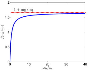
Figure 1: (Color online) Geometric function $f\left(\omega_{\text{Ir}}/\omega_{\text{r}}\right)$ reaches its maximum value at $1+m_{\text{B}}/m_{\text{I}}$.

Inspired by the recent experiments A. D. Lercher et al. (2011); Spethmann et al. (2012a, b); Hohmann et al. (2015), we propose and analyze a quasi one-dimensional model of a hybrid system, which consists of a single ${}^{133}\text{Cs}$ impurity in a ${}^{87}\text{Rb}$ Bose-Einstein condensate. To this end, we start with defining the underlying quasi-1D model in Sec. II. As a result the effective one-dimensional interspecies coupling strength depends not only on the three-dimensional s-wave scattering length, but also on the transversal trap frequencies of cesium and rubidium, respectively. In the same section, we determine the equilibrium phase diagram spanned by the intra- and inter-species coupling strength, and specify the regions where the impurity is localized at the trap center or expelled to the condensate border. Afterwards in Sec. III, we show for the former case that the impurity imprint upon the condensate wave function is either a bump or a dip, depending upon whether the effective impurity-BEC coupling strength is attractive or repulsive. Conversely, due to the presence of the condensate, the effective mass of the impurity turns out to depend quadratically upon a small interspecies coupling strength. Subsequently, Sec. IV discusses the dynamics of the impurity imprint upon the condensate wave function for two quench scenarios. After having released the trap, the resulting time-of-flight expansion shows that the impurity imprint marginally decreases for an attractive s-wave coupling but decreases for a repulsive s-wave scattering with a characteristic time scale which decreases with increasing the interspecies coupling strength. Furthermore, we investigate the emergence of white-shock waves or gray/dark bi-solitons when the initial negative or positive interspecies coupling constant is switched off. Section V summarizes our findings for the proposed quasi 1D model system in view of a possible experimental realization. Finally, in Appendix A we derive for the quasi one-dimensional model the two underlying differential equations (1DDEs) for the condensate and the impurity wave function from a three-dimensional setting.

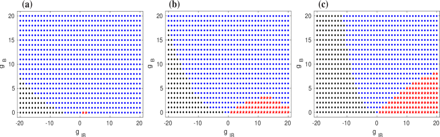
Figure 2: (Color online) Equilibrium phase diagram spanned by $g_{\text{B}}$ and $g_{\text{IB}}$ for (a) $N_{\text{B}}=20$ (b) $N_{\text{B}}=200$ and (c) $N_{\text{B}}=800$. Impurity is localized at trap center (blue) or expelled to the condensate border (red) together with unstable region (black) in dimensionless units.

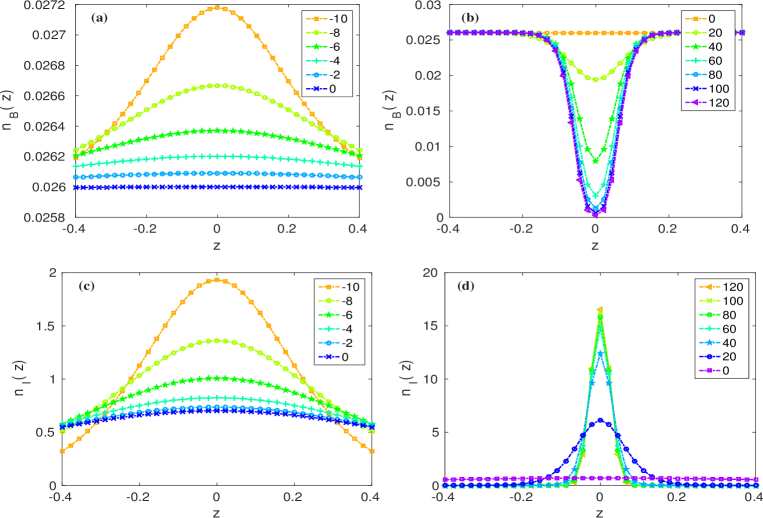
Figure 3: (Color online) Numerical density profile of BEC (a-b) and impurity (c-d) for two-particle Rb-Rb coupling constant value $G_{\text{B}}=16000$ and for interspecies coupling constants $g_{\text{IB}}$ which increases from top to bottom according to the inlets. For increasing negative values of $g_{\text{IB}}$ the impurity-induced bump (a) in the condensate wave function decreases, whereas for positive values the corresponding dip (b) increases in dimensionless units.

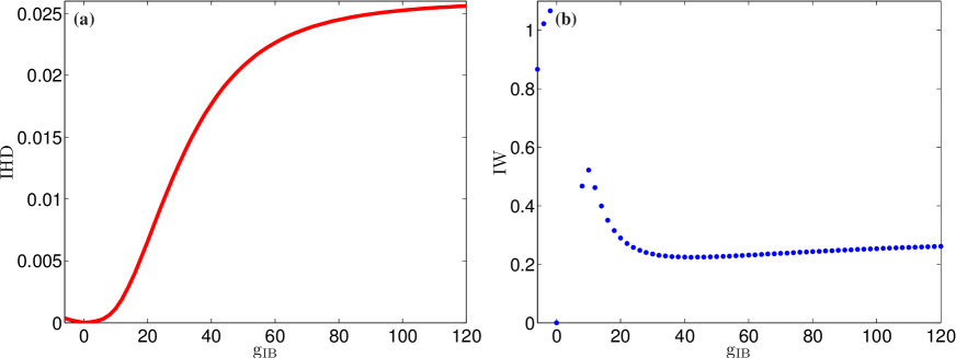
Figure 4: (Color online) (a) Height/depth and (b) width of impurity bump/dip according to Eqs. (12)–(14) versus impurity-BEC coupling constant $g_{\text{IB}}$ for the BEC coupling constant $G_{\text{B}}=16000$ calculated numerically by solving 1DDEs (6) and (7) in dimensionless units.

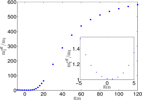
Figure 5: (Color online) Effective mass of ${}^{133}\text{Cs}$ impurity versus the impurity-BEC coupling strength $g_{\text{IB}}$. Inlet shows that effective mass increases quadratically for small impurity-BEC coupling strength $g_{\text{IB}}$ in dimensionless units.

II Quasi 1D model

We start with considering a BEC and an impurity confined in a harmonic trap. In case of a strong transversal confinement one obtains an effective quasi one-dimensional model which is described by two-coupled one-dimensional differential equations for the underlying condensate and impurity wave function $\psi_{\text{B}}\left(z,t\right)$ and $\psi_{\text{I}}(z,t)$, respectively. Appendix A outlines how the one-dimensional Lagrangian density (20) is obtained from an original three-dimensional setting by integrating out the two transversal degrees of freedom. The Euler-Lagrangian equations (21) then reduce to the two coupled one-dimensional differential equations (1DDEs):

$$i\hbar\frac{\partial}{\partial t}\psi_{\text{B}}\left(z,t\right) =\left\{-\frac{\hbar^{2}}{2m_{\text{B}}}\frac{\partial^{2}}{\partial z^{2}}+\frac{m_{\text{B}}\omega_{\text{z}}^{2}}{2}z^{2}+G_{\text{IB}}\parallel\psi_{\text{I}}(z,t)\parallel^{2}\right.$$

$$+G_{\text{B}}\parallel\psi_{\text{B}}\left(z,t\right)\parallel^{2}\biggr{\}}\psi_{\text{B}}\left(z,t\right),$$ (1)

$$i\hbar\frac{\partial}{\partial t}\psi_{\text{I}}(z,t) =\left\{-\frac{\hbar^{2}}{2m_{\text{I}}}\frac{\partial^{2}}{\partial z^{2}}+\frac{m_{\text{I}}\omega_{\text{Iz}}^{2}}{2}+G_{\text{BI}}\parallel\psi_{\text{B}}\left(z,t\right)\parallel^{2}\right\}$$

$$\times\psi_{\text{I}}(z,t).$$ (2)

On the right-hand side of Eqs. (1) and (2) the first term represents the kinetic energy of the BEC(impurity) atoms with mass $m_{\text{B}}$($m_{\text{I}}$), the second term describes the potential energy term, the third term stands for the impurity-BEC coupling with the respective strengths $G_{\text{IB}}=g_{\text{IB}}$, $G_{\text{BI}}=N_{\text{B}}g_{\text{IB}}$, and the last term in (1) represents the Rb-Rb two-particle interaction with strength $G_{\text{B}}=N_{\text{B}}g_{\text{B}}$. In Appendix A it is determined how $g_{\text{B}}$ and $g_{\text{IB}}$ depend on the s-wave scattering lengths $a_{\text{B}}$ and $a_{\text{IB}}$. For intraspecies coupling one gets

$$g_{\text{B}} =2a_{\text{B}}\hbar\omega_{\text{r}},$$ (3)

whereas for interspecies coupling one obtains

$$g_{\text{IB}} =2a_{\text{IB}}\hbar\omega_{\text{r}}f\left(\frac{\omega_{\text{Ir}}}{\omega_{\text{r}}}\right).$$ (4)

Here the geometric function

$$f\left(\frac{\omega_{\text{Ir}}}{\omega_{\text{r}}}\right) =\frac{1+\left(m_{\text{B}}/m_{\text{I}}\right)}{1+\left(m_{\text{B}}\omega_{\text{r}}\right)/\left(m_{\text{I}}\omega_{\text{Ir}}\right)},$$ (5)

depends on the ratio of the trap frequencies as depicted in Fig. 1. Thus, $f\left(\omega_{\text{Ir}}/\omega_{\text{r}}\right)$ is monotonously increasing, equals to one for the present case $\omega_{\text{Ir}}=\omega_{\text{r}}$, and reaches its maximum value at $1+m_{\text{B}}/m_{\text{I}}$ for the frequency ratio of about $\omega_{\text{Ir}}/\omega_{\text{r}}\geq 20$. In order to vary the impurity-BEC coupling strength there are, in principle, two possibilities according to Eq. (5): either the ratio of the radial trap frequencies is tuned as shown in Fig. 1, or the s-wave scattering length $a_{\text{IB}}$ is modified with the use of a Feshbach resonance A. D. Lercher et al. (2011); Pilch et al. (2009); Takekoshi et al. (2012). In order to make Eqs. (1) and (2) dimensionless we introduce the dimensionless time as $\tilde{t}=\omega_{\text{z}}t$, the dimensionless coordinate $\tilde{z}=z/l_{\text{z}}$, and the dimensionless wave function $\tilde{\psi}=\psi\sqrt{l_{\text{z}}}$ with the oscillator length $l_{\text{z}}=\sqrt{\hbar/(m_{\text{B}}\omega_{\text{z}})}$. With this Eqs. (1) and (2) can be rewritten in the form

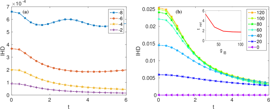
Figure 6: (Color online) Impurity imprint height/depth after having released the trap versus time for (a) increasing negative and (b) decreasing positive values of impurity-BEC coupling constant $g_{\text{IB}}$ from top to bottom. Inlet: relaxation time $t_{\text{rel}}$ decreases with increasing $g_{\text{IB}}$ in dimensionless units.

$$i\frac{\partial}{\partial\tilde{t}}\tilde{\psi}_{\text{B}}\left(\tilde{z},\tilde{t}\right) =\left\{-\frac{1}{2}\frac{\partial^{2}}{\partial\tilde{z}^{2}}+\frac{\tilde{z}^{2}}{2}+\tilde{G}_{\text{IB}}\parallel\tilde{\psi}_{\text{I}}(\tilde{z},\tilde{t})\parallel^{2}\right.$$

$$+\tilde{G}_{\text{B}}\parallel\tilde{\psi}_{\text{B}}\left(\tilde{z},\tilde{t}\right)\parallel^{2}\biggr{\}}\tilde{\psi}_{\text{B}}\left(\tilde{z},\tilde{t}\right),$$ (6)

$$i\frac{\partial}{\partial\tilde{t}}\tilde{\psi}_{\text{I}}(\tilde{z},\tilde{t}) =\left\{-\frac{\tilde{\alpha}^{2}}{2}\frac{\partial^{2}}{\partial\tilde{z}^{2}}+\frac{\tilde{z}^{2}}{2\tilde{\alpha}^{2}}+\tilde{G}_{\text{BI}}\parallel\tilde{\psi}_{\text{B}}(\tilde{z},\tilde{t})\parallel^{2}\right\}$$

$$\times\tilde{\psi}_{\text{I}}(\tilde{z},\tilde{t}),$$ (7)

where we have $\tilde{G}_{\text{B}}=N_{\text{B}}\tilde{g}_{\text{B}}$, $\tilde{G}_{\text{IB}}=\tilde{g}_{\text{IB}}$ and $\tilde{G}_{\text{BI}}=N_{\text{B}}\tilde{g}_{\text{IB}}$ with $\tilde{g}_{\text{B}}=g_{\text{B}}/\left(\hbar\omega_{\text{z}}l_{\text{z}}\right)$, and $\tilde{g}_{\text{IB}}=g_{\text{IB}}/\left(\hbar\omega_{\text{z}}l_{\text{z}}\right)$. Here $\tilde{\alpha}=l_{\text{Iz}}/l_{\text{z}}$ defines the ratio of the two oscillator lengths. Thus, we can summarize that Eq. (6) is nothing but a standard Gross-Piteavskii equation with an additional potential stemming from the impurity, whereas Eq. (7) is a typical Schrödinger wave equation with a potential originating from the BEC. From here on, we will drop the tildes for simplicity.

Typically, a mixture of two species can occur in two different states, either it is miscible, i.e. both species overlap, or it is immiscible, i.e. the two species do not overlap Pu and Bigelow (1998); Sartori and Recati (2013). In our case the equilibrium phase diagram is spanned by the coupling strengths $g_{\text{B}}$ and $g_{\text{IB}}$ and contains a region, where the impurity is localized at the center, and another one, where the impurity is expelled to be localized at the border of the condensate. Note that a similar equilibrium phase diagram was studied for the homogeneous case with attractive interspecies s-wave scattering lengths in Ref. Kalas and Blume (2006). In order to investigate the physical regions of interest for our proposed model, we solve the two coupled 1DDEs (6) and (7) in imaginary time numerically by using the split-operator method Vudragović et al. (2012); Kumar et al. (2015); Lončar et al. (2016); Satarić et al. (2016), which yields the equilibrium phase diagram Fig. 2. The blue region shows where the impurity is localized at the center of the BEC, the red region depicts that the impurity is displaced from the center to the border of the condensate, and finally, the black region represents the unstable region where impurity and condensate do not coexist.

In the rest of the paper, we are interested into the localization of the impurity at the center of the BEC, therefore, from now on, we only focus on the blue region in the equilibrium phase diagram of Fig. 2. In particular, we consider that the BEC consists of $N_{\text{B}}=800$ ${}^{87}\text{Rb}$ atoms, for the dimensionless intraspecies couplings constant we assume $G_{\text{B}}=16000$, and we let the ratio of the two oscillator lengths $\alpha=l_{\text{Iz}}/l_{\text{z}}$ to have the value 0.808.

III Impurity Imprint Upon Stationary Condensate Wave Function

In order to determine the impurity imprint on the condensate wave function in equilibrium we solve the two coupled 1DDEs numerically in imaginary time. In this way we find that the impurity leads to a bump/hole in the BEC density at the trap center for negative/positive values of $g_{\text{IB}}$ as shown in Fig. 3. For increasing the attractive/repulsive interspecies coupling strength the bump/dip upon the condensate decreases/increases. For the repulsive interspecies coupling strength, the impurity drills a dip in the BEC density which gets deeper and deeper until no more BEC atoms remain in the trap center and, finally, the BEC fully fragments into two parts as shown in Fig. 3(b) at the characteristic value $g_{\text{IBc}}=110$. The width/height of the impurity wave function decreases/increases for increasing interspecies coupling constant $\left|g_{\text{IB}}\right|$, respectively, as shown in Fig. 3(c-d).

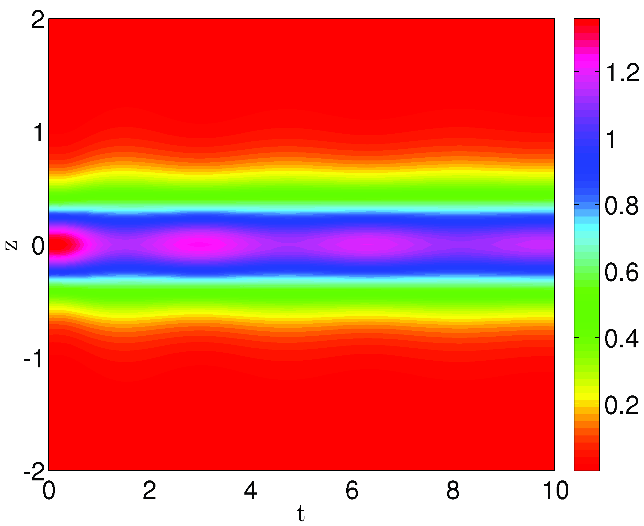
Figure 7: (Color online) Dynamics of impurity density represented in color scale after having switched off the harmonic trap for initial $g_{\text{IB}}$=-8 for the BEC coupling strength $G_{\text{B}}=16000$ in dimensionless units.

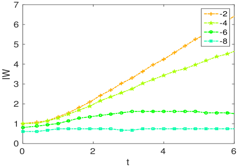
Figure 8: (Color online) Impurity imprint width after having released the trap versus time for decreasing positive values of impurity-BEC coupling constant $g_{\text{IB}}$ from top to bottom in dimensionless units.

In view of a more detailed comparison, we describe the impurity imprint upon the condensate wave function $\psi_{\text{B}}(z)$ by the following two quantities. The first one is the impurity height/depth

$$\begin{array}[]{r@{}l@{\,}l}\text{IHD}=\left\{\begin{array}[]{r@{}l@{\,}l}\parallel\psi_{\text{B}}\left(0\right)\parallel_{g_{\text{IB}}}^{2}-\parallel\psi_{\text{B}}\left(0\right)\parallel_{g_{\text{IB}}=0}^{2}\qquad g_{\text{IB}}\leq 0\\ \\ \text{Max}\left(\parallel\psi_{\text{B}}\left(z\right)\parallel_{g_{\text{IB}}}^{2}\right)-\parallel\psi_{\text{B}}\left(0\right)\parallel_{g_{\text{IB}}}^{2}\qquad g_{\text{IB}}\geq 0\end{array}\right.\end{array}$$ (12)

and the second one is the impurity width IW, which we define as follows. For $g_{\text{IB}}\leq 0$ we use the full width half maximum

$$\parallel\psi\left(\text{IW}/2\right)\parallel_{g_{\text{IB}}}^{2}=\frac{\parallel\psi_{\text{B}}\left(0\right)\parallel_{g_{\text{IB}}}^{2}+\parallel\psi_{\text{B}}\left(0\right)\parallel_{g_{\text{IB}}=0}^{2}}{2}\,\>g_{\text{IB}}\leq 0\,,$$ (13)

whereas for $g_{\text{IB}}\geq 0$ we define the equivalent width Carroll and Ostlie (2007):

$$\text{IW}=\frac{2I_{\text{0}}z_{\text{Max}}-\intop_{-z_{\text{Max}}}^{z_{\text{Max}}}\parallel\psi_{\text{B}}\left(z\right)\parallel_{g_{\text{IB}}}^{2}dz}{I_{\text{0}}-\parallel\psi_{\text{B}}\left(0\right)\parallel_{g_{\text{IB}}}^{2}}\quad g_{\text{IB}}\geq 0\,,$$ (14)

where we have $I_{\text{0}}=\text{Max}\left(\parallel\psi_{\text{B}}\left(z\right)\parallel_{g_{\text{IB}}}^{2}\right)$. In Fig. 4(a) we plot the IHD for $g_{\text{IB}}>-10$, while $g_{\text{IB}}<-10$ is not a valid region for $g_{\text{B}}=20$ according to Fig. 2(c). From Figure 4(a) we read off that for $g_{\text{IB}}=0$, i.e. when there is no impurity present, the impurity height/depth vanishes. The IHD quadratically increases for the repulsive interspecies coupling strength $0<g_{\text{IB}}<60$ and partially fragments the BEC until it reaches its marginally saturated value $\text{IHDc}\approx 0.025$ for the characteristic interspecies coupling strength $g_{\text{IBc}}=110$. In the case of $g_{\text{IB}}>g_{\text{IBc}}$, the impurity fully fragments the BEC into two parts as shown in Fig. 3(b). The impurity imprint width increases abruptly just before/after $g_{\text{IB}}=0$ for attractive/repulsive interspecies coupling strength, respectively, as shown in Fig. 4(b). For an increasing repulsive impurity-BEC coupling strength the impurity width then decreases until it reaches the interspecies coupling strength $g_{\text{IB}}=30$, later on it marginally increases until the characteristic interspecies coupling strength $g_{\text{IBc}}=110$, where we have $\text{IWc}\approx 0.23$.

The effective mass of the impurity is defined as $m_{\text{I}}^{\text{eff}}=\hbar/\left(l_{\text{Iz}}^{2}\omega_{\text{z}}\right)$, where the impurity oscillator length $l_{\text{Iz}}=\sqrt{2}\sigma$ follows from the standard deviation $\sigma=\sqrt{<z^{2}>-<z>^{2}}$, with $<\bullet>=\int\bullet\left|\psi_{\text{I}}(z)\right|^{2}dz$ denoting the expectation value. Figure 5 shows the ratio of the effective mass of the ${}^{133}\text{Cs}$ impurity with respect to the bare mass $m_{\text{I}}$, which increases quadratically for interspecies coupling strength $-5<g_{\text{IB}}<5$ as shown in the inlet of Fig. 5, and becomes marginally saturated for interspecies coupling strength $g_{\text{IB}}>g_{\text{IBc}}$. Note that our results for the effective mass of the impurity are restricted to the mean-field regime. In order to go beyond and include the impact of quantum fluctuations, one would need to investigate polaron physics Tempere et al. (2009); Casteels et al. (2011); Santamore and Timmermans (2011); Grusdt and Demler (2015).

IV Impurity Imprint Upon Condensate Dynamics

In an experiment, any imprint of the impurity upon the condensate wave function could only be detected dynamically. Thus, it is of high interest to study theoretically whether the impurity imprint, which we have found and analyzed for the stationary case in the previous section, remains present also during the dynamical evolution of the condensate wave function. To this end, we explore two quench scenarios numerically in more detail. The first one is the standard time-of-flight (TOF) expansion after having switched off the external trap when the interspecies interaction is still present. In the second case we consider the inverted situation that the impurity-BEC interaction is suddenly switched off within a remaining harmonic confinement, which turns out to give rise to the emergence of wave packets or bi-solitons depending on whether the initial interspecies interaction strength is attractive or repulsive.

IV.1 Time-of-Flight Expansion

Time-of-flight (TOF) absorption pictures represent an important diagnostic tool to analyze dilute quantum gases since the field’s inception. By suddenly turning off the magnetic trap, the atom cloud expands non-ballistically with a dynamics which is determined by both the momentum distribution of the atoms at the instance, when the confining potential is switched off, and by inter-atomic interactions Mewes et al. (1996); Inouye et al. (1999). We have investigated the time-of-flight expansion dynamics of the BEC with impurity by solving numerically the two coupled 1DDEs (6), (7) and analyzing the resulting evolution of both the condensate and the impurity wave function. It turns out that, despite the continuous broadening of the condensate density, its impurity imprint remains qualitatively preserved both for attractive and repulsive interspecies interaction strengths, respectively. Therefore, we focus a more quantitative discussion upon the dynamics of the corresponding impurity height/depth and width.

For an attractive Rb-Cs coupling strength, it turns out that the impurity imprint even remains approximately constant in the time-of-flight, as is shown explicitly in Fig. 6 (a) for the IHD, which marginally decreases for $t\gg 0$. As shown in Fig. 6 (a) for smaller attractive interspecies coupling strength, we observe the crumbling breathing of the impurity upon IHD as discussed recently for the Bose-Hubbard model Peotta et al. (2013). For the attractive interspecies coupling strength $g_{\text{IB}}=-8$ the dynamics of the impurity density is shown in Fig. 7, which clearly reflects the crumbling breathing of the impurity at the center of the BEC. In case of the IW, we find that the IW starts increasing marginally for smaller values of attractive interspecies coupling strength and increases linearly for larger attractive interspecies coupling strength $g_{\text{IB}}$ as shown in Fig. 8.

In case of a repulsive interspecies interaction, the IHD decays with a characteristic time scale as shown in Fig. 6(b). Defining that relaxation time $t_{\textrm{rel}}$ according to $\textrm{IHD}(t_{\textrm{rel}})=\textrm{IHD}(0)/2$, the inlet reveals that the impurity imprint depth relaxes with a shorter time scale for increasing repulsive impurity-BEC coupling strength. This physical picture is confirmed by the time-of-flight evolution of the depleted density depicted in Fig. 9. At the beginning of TOF the impurity-imprint remains at first constant, then the imprint width expands and the imprint height decays faster for a larger interspecies coupling strength. In Fig. 9 we plotted the time-of-flight of the depleted density of the BEC for two cases. For the repulsive interspecies coupling strength $g_{\text{IB}}=20$ we observe that the impurity imprint decays marginally from its equilibrium value as shown in Fig. 6(b) and the impurity remains localized at the trap center as shown in Fig. 9(a). On the other hand, for the larger value of the repulsive interspecies coupling strength $g_{\text{IB}}=80$, the impurity imprint decays from its equilibrium value as shown in Fig. 6(b) and at the same time the impurity is expelled from the center of the BEC as shown in Fig. 9(b). With this we conclude that for a small enough repulsive interspecies coupling strengths the impurity survives in the center of the BEC for larger times.

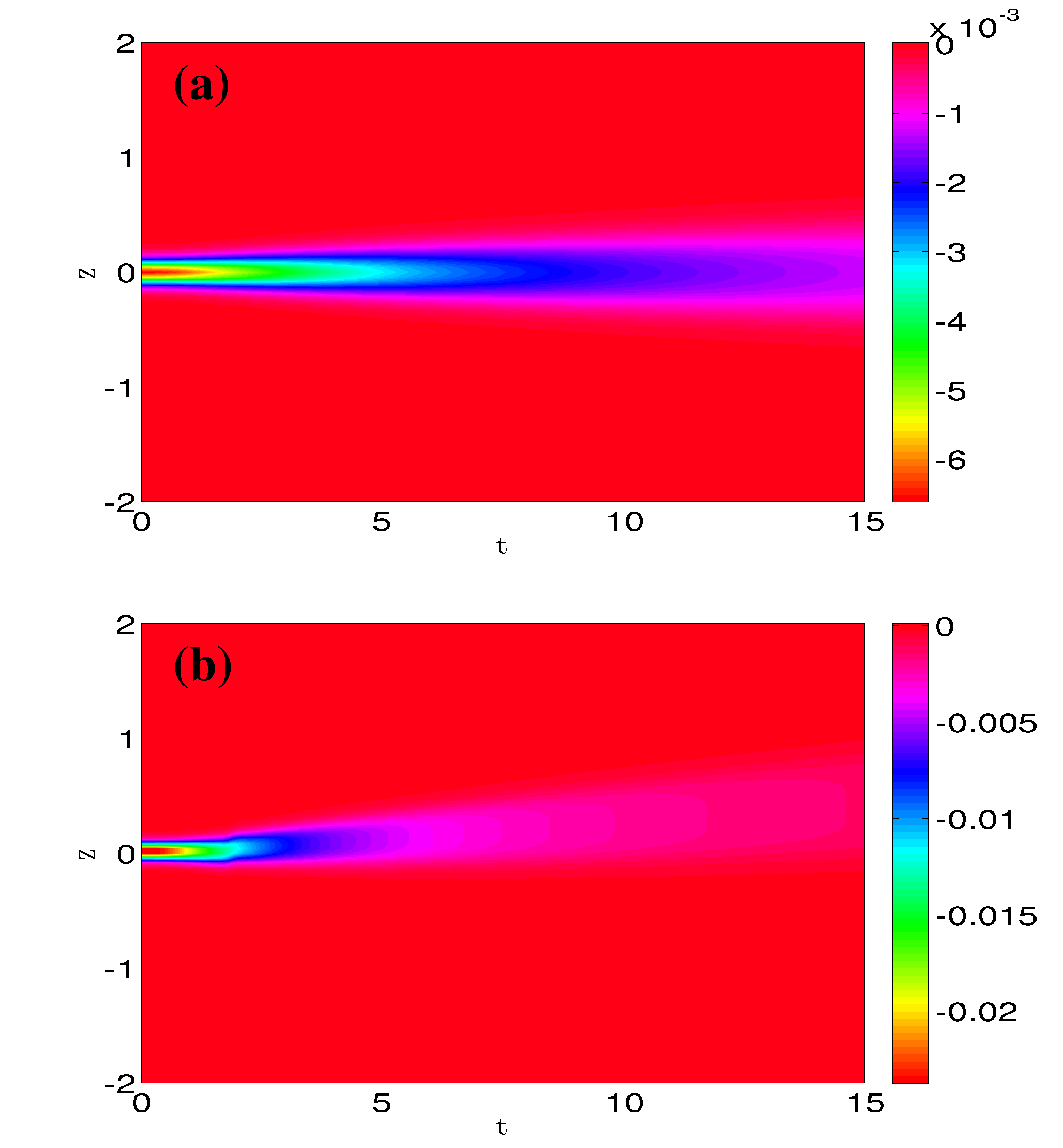
Figure 9: (Color online) Coherent matter-wave time-of-flight evolution of the depleted density $\left\|\psi_{\text{B}}\left(z,t\right)\right\|_{\text{\text{DD}}}^{2}=\left\|\psi_{\text{B}}\left(z,t\right)\right\|_{\text{$g_{\text{IB}}$}}^{2}-\left\|\psi_{\text{B}}\left(z,t\right)\right\|_{\text{$g_{\text{IB}}=0$}}^{2}$ represented in color scale after having switched off the trap for the BEC coupling constant $G_{\text{B}}=16000$: (a) $g_{\text{IB}}=20$ and (b) $g_{\text{IB}}=80$ in dimensionless units.

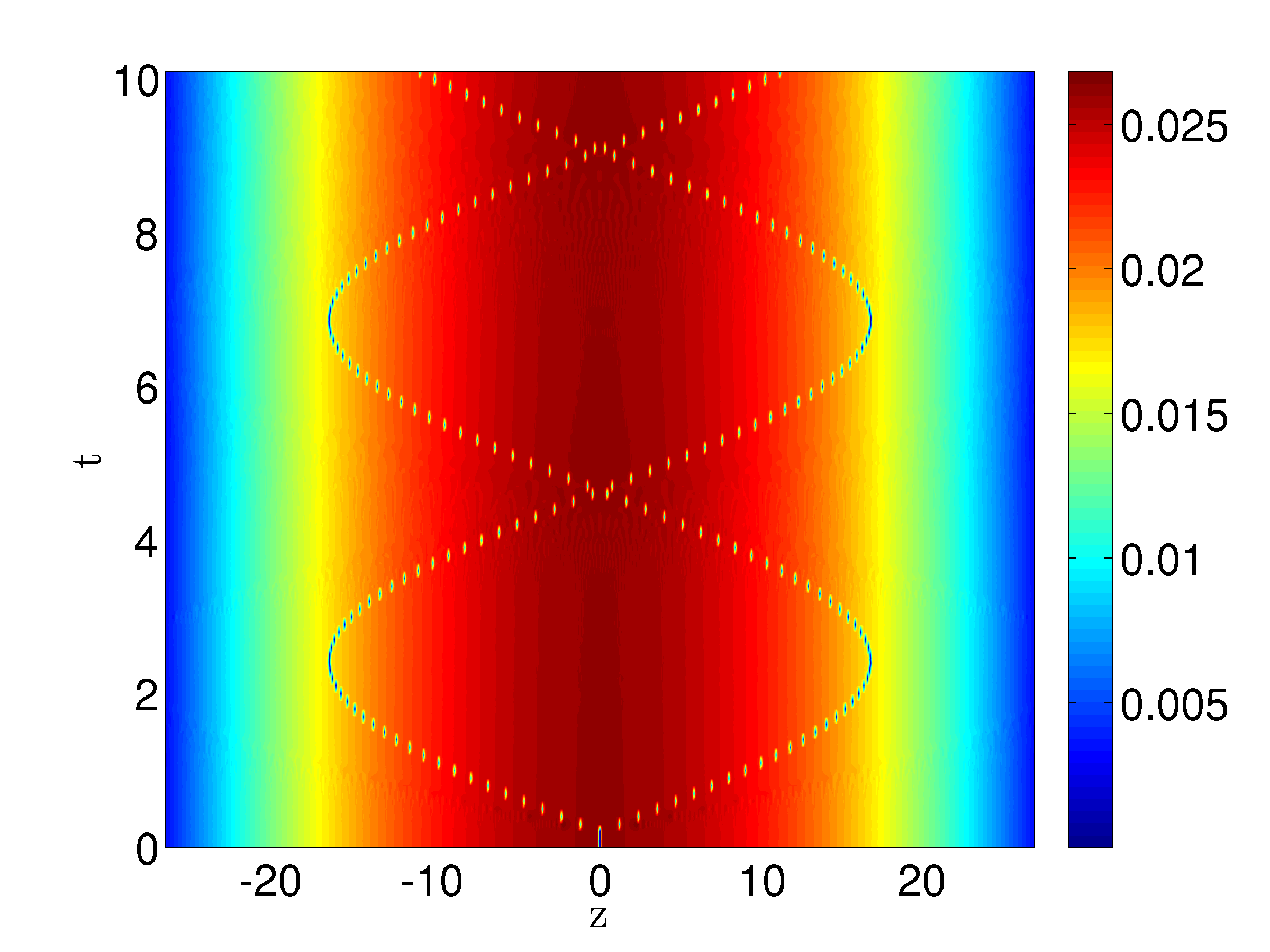
Figure 10: (Color online) Density profile of BEC represented in color scale after having switched off the impurity-BEC coupling constant for initial $g_{\text{IB}}$=120 for the BEC coupling constant $G_{\text{B}}=16000$ in dimensionless units.

IV.2 Wave Packets Versus Solitons

Due to their quantum coherence, BECs exhibit rich and complex dynamic patterns, which range from the celebrated matter-wave interference of two colliding condensates Andrews et al. (1997a) over Faraday waves Engels et al. (2007); Balaž and Nicolin (2012) to the particle-like excitations of solitons Reinhardt and Clark (1997); Kivshar and Luther-Davies (1998); Scott et al. (1998); Busch and Anglin (2000); Ruostekoski et al. (2001); C. Becker et al. (2008); Shomroni et al. (2009); Akram and Pelster (2015, 2016). For our proposed quasi 1D model of a BEC with an impurity we investigated the dynamics of the condensate wave function which emerges after having switched off the interspecies coupling strength. Both for an initial attractive and repulsive interspecies coupling strength $g_{\text{IB}}$ we observe that two excitations of the condensate are created at the impurity position, which travel in opposite direction with the same center-of-mass speed, are reflected at the trap boundaries and then collide at the impurity position as shown exemplarily in Fig. 10 for the initial $g_{\text{IB}}$=120 and $G_{\text{B}}=16000$. These excitations qualitatively retain their shape despite the collision at the impurity position. All these findings are not yet conclusive to decide whether these excitations represent wave packets in the absence of dispersion or solitons. Therefore, we investigate their dynamics in more detail, by determining their center-of-mass motion via Akram and Pelster (2015)

$$\bar{z}_{{\rm{L,R}}}\left(t\right)=\frac{\int_{-\infty,0}^{0,\infty}z\left(\parallel\psi_{\text{B}}\left(z,t\right)\parallel_{g_{\text{IB}}}^{2}-\parallel\psi_{\text{B}}\left(z,t\right)\parallel_{g_{\text{IB}}=0}^{2}\right)dz}{\int_{-\infty,0}^{0,\infty}\left(\parallel\psi_{\text{B}}\left(z,t\right)\parallel_{g_{\text{IB}}}^{2}-\parallel\psi_{\text{B}}\left(z,t\right)\parallel_{g_{\text{IB}}=0}^{2}\right)dz}\,,$$ (15)

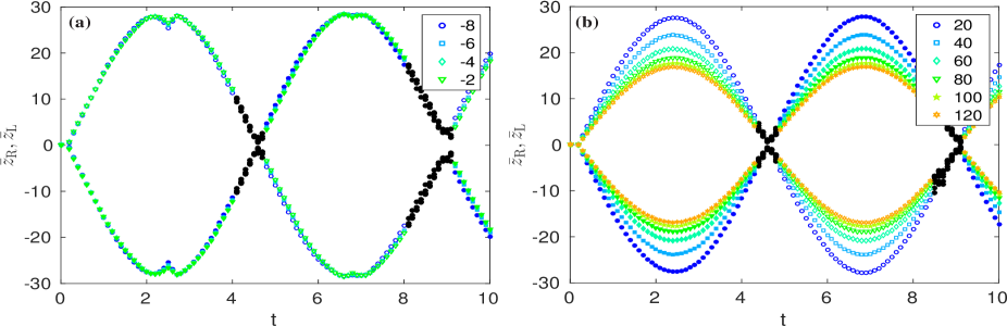
Figure 11: (Color online) Center of mass positions of excitations $\bar{z}_{{\rm L}}$ (filled circles) and $\bar{z}_{{\rm R}}$ (empty circles) according to Eq. (15) versus time after having switched off (a) negative decreasing and (b) positive increasing values of $g_{\text{IB}}$ from top to bottom in dimensionless units. Black filled circles represent the region of colliding excitations, where mean positions are not perfectly detectable.

which are plotted in Fig. 11. Note that the mean positions $\bar{z}_{{\rm{L}}}$ and $\bar{z}_{{\rm{R}}}$ of the excitations are uncertain in the region where they collide. Nevertheless Fig. 11 demonstrates that the excitations oscillate with the frequency $\omega=2\pi\times 35.7~{}{\rm Hz}$ irrespective of sign and size of $g_{\text{IB}}$. As we have assumed the trap frequency $\omega_{{\rm z}}=2\pi\times 50~{}{\rm Hz}$, we obtain the ratio $\omega/\omega_{{\rm z}}\approx 0.714$, which is quite close to $\omega/\omega_{{\rm z}}=1/\sqrt{2}\approx 0.707$. Despite these similarities of the cases of an initial attractive and repulsive interspecies coupling constant $g_{\text{IB}}$, we observe one significant difference. Whereas the oscillation amplitudes of the excitations do not depend on the value of the initial $g_{\text{IB}}<0$ according to Fig. 11 (a), we find decreasing oscillation amplitudes of the excitations with increasing the initial $g_{\text{IB}}>0$ in Fig. 11 b). Such an amplitude dependence on the initial condition is characteristic for gray/dark solitons according to Ref. Busch and Anglin (2000). This particle-like interpretation of the excitations agrees with the other theoretical prediction of Ref. Busch and Anglin (2000) that gray/dark solitons oscillate in a harmonic confinement with the frequency $\omega/\omega_{{\rm z}}=1/\sqrt{2}$, which was already confirmed in the Hamburg experiment of Ref. C. Becker et al. (2008) and is also seen in Fig. 11. Conversely, for an initial attractive interspecies coupling constant the excitations can not be identified with bright solitons as the dynamics is governed by a GPE with a repulsive two-particle interaction. Here the excitations have to be interpreted as wave packets which move without any dispersion, thus, for $g_{\text{IB}}<0$ the excitations propagate like sound waves in the BEC Andrews et al. (1997b); Akram and Pelster (2015, 2016). Thus, we conclude that switching off the interspecies coupling constant leads for $g_{\text{IB}}<0$ and $g_{\text{IB}}>0$ to physically different situations. For an initial attractive RbCs coupling constant we generate wave packets which correspond to white-shock waves Damski (2006), whereas for the corresponding repulsive case bi-solitons emerge K.E. Strecker et al. (2002); Al Khawaja et al. (2002), which are due to the collision of the two partially/fully fragmented parts of the condensate. When the shock wave approaches the trap boundary, it penetrates into the trap potential, which leads to a change of its shape, later it recovers its shape. Therefore we see a small kink in the center of mass position amplitude at time $t\thicksim 2.5$ as shown in Fig. 11(a). On the other hand the solitary wave is characterized by preserving its shape so it is reflected back from the potential boundary without changing its shape. Thus we do not see any kink in Fig. 11(b). Note that it can be shown in our proposed system that gray bi-solitons are generated for a partially fragmented BEC, i.e. the impurity-BEC coupling strength $g_{\text{IB}}<g_{\text{IBc}}$. On the other hand the dark bi-solitons turn out to be only generated for $g_{\text{IB}}>g_{\text{IBc}}$, where the BEC is fully fragmented into two parts at equilibrium. Recently, we have observed that bi-solitons trains are generated in the traditional harmonic trap with an additional dimple trap Akram and Pelster (2015). We emphasize that beside many practical application of the impurity-BEC system, someone can also generate solitons by considering an impurity as a drilling appliance to fragment the BEC, which allows to study solitons physics in the condensate.

V Summary and Conclusion

In the present work we studied within a quasi 1D model numerically how a single impurity in the center of a trapped BEC affects the condensate wave function. At first, we investigated the equilibrium properties of that hybrid system by numerically solving the underlying two coupled 1DDEs (6) and (7) with the imaginary-time propagation method. For an increasing attractive/repulsive Rb-Cs interaction strength it turns out that the impurity imprint bump/dip decreases/increases quadratically and reaches its marginally saturated value after $g_{\text{IBc}}=110$. Later we found that the impurity imprint width increases abruptly for increasing the attractive/repulsive Rb-Cs interaction strength, but for the repulsive case it reaches a marginally saturated value for $g_{\text{IB}}>g_{\text{IBc}}$. Beyond the characteristic value $g_{\text{IBc}}$, the BEC fragments into two parts and, if $g_{\text{IB}}$ is increased beyond $g_{\text{IBc}}$, the impurity yields a condensate wave function whose impurity width increases further, although the impurity height/depth remains constant. Afterwards, we investigated the impurity imprint upon the condensate dynamics for two quench scenarios.

At first, we considered the release of the harmonic confinement, which leads to a time-of-flight expansion and found that the impurity imprint upon the condensate decays slowly for small valves of the attractive/repulsive interspecies coupling strength. This result suggests that it might be experimentally easier to observe the impurity imprint for small attractive/repulsive coupling constant $g_{\text{IB}}$. We also observed the decaying breathing of the impurity at the center of the condensate for small attractive Rb-Cs coupling strength. Additionally, we found for stronger repulsive interspecies coupling strength that the ${}^{87}\text{Rb}$ atoms repel the single ${}^{133}\text{Cs}$ impurity from the center. In an experiment one has to take into account that inelastic collisions lead to two- and three-body losses of the condensate atoms Cornish et al. (2000); Carretero-González et al. (2008). As such inelastic collisions are enhanced for a higher BEC density, they play a vital role for an attractive interspecies coupling, when the condensate density has a bump at the impurity position, but are negligible in the repulsive case with the dip in the wave function.

In addition, we analyzed the condensate dynamics after having switched off the interspecies coupling strength. This case turned out to be an interesting laboratory in order to study the physical similarities and differences of bright shock waves and gray/dark bi-solitons, which emerge for an initial negative and positive interspecies coupling constant $g_{\text{IB}}$, respectively. We consider the astonishing observation, that the oscillation frequencies of both the shock waves and the soliton coincide, to be an artifact of the harmonic confinement. Additionally, we also found that the generation of gray/dark bi-solitons is a generic phenomenon on collisions of partially/fully fragmented BEC, respectively, which is strongly depending upon the equilibrium values of the impurity wave function height and width.

Acknowledgment

We thank James Anglin, Antun Balaž, Herwig Ott, Ednilson Santos, and Artur Widera for insightful comments. Furthermore, we gratefully acknowledge financial support from the German Academic Exchange Service (DAAD). This work was also supported in part by the German-Brazilian DAAD-CAPES program under the project name “Dynamics of Bose-Einstein Condensates Induced by Modulation of System Parameters” and by the German Research Foundation (DFG) via the Collaborative Research Center SFB/TR49 “Condensed Matter Systems with Variable Many-Body Interactions”.

Appendix A  

We start with the fact that the underlying equations for describing an impurity immersed in a BEC can be formulated in terms of the Hamilton principle of least action with the action functional $\mathcal{A}_{\text{3D}}=\int dt\int\mathcal{L_{\text{3D}}}\;d^{3}r$, where the Lagrangian density reads for three dimensions

$$\mathcal{L}_{\text{3D}}=\sum_{j=\text{B,I}}N_{\text{j}}\biggl{\{}\frac{i\hbar}{2}\left[\psi_{\text{j}}^{\star}\left(\mathbf{r},t\right)\frac{\partial\psi_{\text{j}}\left(\mathbf{r},t\right)}{\partial t}-\psi_{\text{j}}\left(\mathbf{r},t\right)\frac{\partial\psi_{\text{j}}^{\star}\left(\mathbf{r},t\right)}{\partial t}\right]$$

$$+\frac{\hbar^{2}}{2m_{\text{j}}}\psi_{\text{j}}^{\star}\left(\mathbf{r},t\right)\bigtriangleup\psi_{\text{j}}\left(\mathbf{r},t\right)-V_{\text{j}}(\mathbf{r})\psi_{\text{j}}^{\star}\left(\mathbf{r},t\right)\psi_{\text{j}}\left(\mathbf{r},t\right)-\frac{N_{\text{j}}g_{\text{j}}^{\text{3D}}}{2}$$

$$\times\parallel\psi_{\text{j}}\left(\mathbf{r},t\right)\parallel^{4}\biggr{\}}-N_{\text{B}}N_{\text{I}}g_{\text{IB}}^{\text{3D}}\parallel\psi_{\text{I}}\left(\mathbf{r},t\right)\parallel^{2}\parallel\psi_{\text{B}}\left(\mathbf{r},t\right)\parallel^{2}.$$ (16)

Here $\psi_{\text{B}}\left(\mathbf{r},t\right)$ and $\psi_{\text{I}}\left(\mathbf{r},t\right)$ describe the BEC and the impurity wave-function with $\mathbf{r}=\left(x,\;y,\;z\right)$, $V_{\text{B}}(\mathbf{r})=m_{\text{B}}\omega_{\text{z}}^{2}z^{2}/2+m_{\text{B}}\omega_{\text{r}}^{2}\left(x^{2}+y^{2}\right)/2$ and $V_{\text{I}}\left(\mathbf{r}\right)=m_{\text{I}}\omega_{\text{Iz}}^{2}z^{2}/2+m_{\text{I}}\omega_{\text{Ir}}^{2}\left(x^{2}+y^{2}\right)/2$ denote the three-dimensional harmonic potential for the bosons and the ${}^{133}\text{Cs}$ impurity. The three-dimensional ${}^{87}\text{Rb}$ coupling constant reads $g_{\text{B}}^{\text{3D}}=4\pi\hbar^{2}a_{\text{B}}/m_{\text{B}}$, where the s-wave scattering length is $a_{\text{B}}=94.7~{}{\rm{a}_{0}}$ with the Bohr radius ${\rm{a}_{0}}$ and $m_{\text{B}}$ stands for the mass of the ${}^{87}\text{Rb}$ atom, while the three-dimensional ${}^{133}\text{Cs}$ coupling constant reads $g_{\text{I}}^{\text{3D}}=0$, because their is only one single ${}^{133}\text{Cs}$ impurity atom present into the system, i.e. $N_{\text{I}}=1$. The three-dimensional effective Rb-Cs coupling constant is $g_{\text{IB}}^{\text{3D}}=2\pi\hbar^{2}a_{\text{IB}}/m_{\text{IB}}$, where $m_{\text{IB}}=m_{\text{I}}m_{\text{B}}/\left(m_{\text{I}}+m_{\text{B}}\right)$ is the reduced mass of two species, $m_{\text{I}}$ is the mass of the ${}^{133}\text{Cs}$ atom, and $a_{\text{IB}}=650~{}{\rm{a}_{0}}$ represents the effective Rb-Cs s-wave scattering length A. D. Lercher et al. (2011). We assume an effective one-dimensional setting with $\omega_{\text{z}}\ll\omega_{\text{r}}$, so we decompose the BEC wave-function $\psi_{\text{B}}(\mathbf{r},t)=\psi_{\text{B}}(z,t)\phi_{\text{B}}(\textbf{ r}_{\perp},t)$ with $\textbf{ r}_{\perp}=\left(x,\;y\right)$ and

$$\phi_{\text{B}}(\textbf{ r}_{\perp},t) = \frac{e^{-\frac{x^{2}+y^{2}}{2l_{\text{r}}^{2}}}}{\sqrt{\pi}l_{\text{r}}}e^{-i\omega_{\text{r}}t}\,.$$ (17)

Furthermore, we assume that the single impurity in the center of the BEC is trapped by a harmonic potential with $\omega_{\text{Iz}}\ll\omega_{\text{Ir}}$. Thus, we perform a similar decomposition of the impurity wave function $\psi_{\text{I}}(\mathbf{r},t)=\psi_{\text{I}}(z,t)\phi_{\text{I}}(\textbf{ r}_{\perp},t)$ with

$$\phi_{\text{I}}(\textbf{ r}_{\perp},t) = \frac{e^{-\frac{x^{2}+y^{2}}{2l_{\text{rI}}^{2}}}}{\sqrt{\pi}l_{\text{rI}}}e^{-i\omega_{\text{rI}}t}\,.$$ (18)

Here $l_{\text{r}}=\sqrt{\hbar/(m_{\text{B}}\omega_{\text{r}})}$ and $l_{\text{Ir}}=\sqrt{\hbar/(m_{\text{I}}\omega_{\text{Ir}})}$ denote the oscillator lengths in radial direction for BEC and impurity. For the experimentally realistic trap frequencies $\omega_{\text{r}}=\omega_{\text{Ir}}=2\pi\times 0.179~{}\text{kHz}\ll\omega_{\text{z}}=\omega_{\text{Iz}}=2\pi\times 0.050~{}\text{kHz}$ Spethmann et al. (2012a) these radial oscillator lengths amount to the values $l_{\text{r}}=15190.8\,{a}_{0}$ and $l_{\text{Ir}}=12279.0\,{a}_{0}$ for BEC and impurity, respectively. In order to distinguish between the weakly interacting quasi-1D and the strongly interacting Tonks-Girardeau regime, Petrov et al. Petrov et al. (2000) introduced a dimensionless quantity which involves both the longitudinal and the transversal trap size as well as the scattering length:

$$\alpha=2a_{\text{B}}\frac{l_{\text{z}}}{l_{\text{r}}^{2}}\,.$$ (19)

By using above mentioned experimental parameters, we get the dimensionless quantity $\alpha=0.023,$ so we are far in the weakly interacting regime, where the Gross-Pitaevskii mean-field theory is applicable, see also Fig. 5 of Ref. Petrov et al. (2004) and Refs. Ketterle and van Druten (1996); Carr et al. (2000). Therefore, we can follow Ref. Kamchatnov (2004) and integrate out the two transversal dimensions of our three-dimensional Lagrangian according to $\mathcal{L}_{\text{1D}}=\int_{-\infty}^{\infty}\int_{-\infty}^{\infty}\mathcal{L}_{\text{3D}}\;dxdy$. After some algebra, the resulting quasi one dimensional Lagrangian reads

$$\mathcal{L}_{\text{1D}}=\sum_{j=\text{B,I}}N_{\text{j}}\biggl{\{}\frac{i\hbar}{2}\left[\psi_{\text{j}}^{\star}\left(z,t\right)\frac{\partial\psi_{\text{j}}\left(z,t\right)}{\partial t}-\psi_{\text{j}}\left(z,t\right)\frac{\partial\psi_{\text{j}}^{\star}\left(z,t\right)}{\partial t}\right]$$

$$+\frac{\hbar^{2}}{2m_{\text{j}}}\psi_{\text{j}}^{\star}\left(z,t\right)\bigtriangleup\psi_{\text{j}}\left(z,t\right)-V_{\text{j}}(z)\psi_{\text{j}}^{\star}\left(z,t\right)\psi_{\text{j}}\left(z,t\right)-\frac{N_{\text{j}}g_{\text{j}}}{2}$$

$$\parallel\psi_{\text{j}}\left(z,t\right)\parallel^{4}\biggr{\}}-N_{\text{B}}N_{\text{I}}g_{\text{IB}}\parallel\psi_{\text{I}}\left(z,t\right)\parallel^{2}\parallel\psi_{\text{B}}\left(z,t\right)\parallel^{2},\!\!\!\!$$ (20)

where $V_{\text{B,I}}\left(z\right)=m_{\text{B,I}}\omega_{\text{z,Iz}}^{2}z^{2}/2$ represents the one-dimensional harmonic potential for the BEC and for the impurity, the one-dimensional intraspecies coupling strength $g_{\text{B}}$ is given by (3) and the interspecies coupling strength $g_{\text{IB}}$ turns out to be (4). The two coupled time dependent differential equations follow from the action $\mathcal{A}_{\text{1D}}=\int_{-\infty}^{\infty}\int_{-\infty}^{\infty}\mathcal{L}_{\text{1D}}dzdt$ and by using the Euler-Lagrangian equation

$$\frac{\partial\mathcal{L}_{\text{1D}}}{\partial\psi_{\text{j}}^{\star}\left(z,t\right)}-\frac{\partial}{\partial z}\frac{\partial\mathcal{L}_{\text{1D}}}{\partial\frac{\partial\psi_{\text{j}}^{\star}\left(z,t\right)}{\partial z}}-\frac{\partial}{\partial t}\frac{\partial\mathcal{L}_{\text{1D}}}{\partial\frac{\partial\psi_{\text{j}}^{\star}\left(z,t\right)}{\partial t}}=0.$$ (21)

Inserting the one-dimensional Lagrangian density (20), after some algebra we obtain the two coupled 1DDEs (1) and (2).

References

- T. Gericke et al. (2008) T. Gericke, P. Wurtz, D. Reitz, T. Langen, and H. Ott, Nature Phys. 4, 949 (2008).
- W. S. Bakr et al. (2009) W. S. Bakr, J. I. Gillen, A. Peng, S. Folling, and M. Greiner, Nature (London) 462, 74 (2009).
- J. F. Sherson et al. (2010) J. F. Sherson, C. Weitenberg, M. Endres, M. Cheneau, I. Bloch, and S. Kuhr, Nature (London) 467, 68 (2010).
- Serwane et al. (2011) F. Serwane, G. Zürn, T. Lompe, T. B. Ottenstein, A. N. Wenz, and S. Jochim, Science 332, 336 (2011).
- A. V. Gorshkov et al. (2010) A. V. Gorshkov, M. Hermele, V. Gurarie, C. Xu, P. S. Julienne, J. Ye, P. Zoller, E. Demler, M. D. Lukin, and A. M. Rey, Nature Phys. 6, 289 (2010).
- Schirotzek et al. (2009) A. Schirotzek, C.-H. Wu, A. Sommer, and M. W. Zwierlein, Phys. Rev. Lett. 102, 230402 (2009).
- Palzer et al. (2009) S. Palzer, C. Zipkes, C. Sias, and M. Köhl, Phys. Rev. Lett. 103, 150601 (2009).
- C. Zipkes et al. (2010) C. Zipkes, S. Palzer, C. Sias, and M. Köhl, Nature (London) 464, 388 (2010).
- Schmid et al. (2010) S. Schmid, A. Härter, and J. H. Denschlag, Phys. Rev. Lett. 105, 133202 (2010).
- Micheli et al. (2004) A. Micheli, A. J. Daley, D. Jaksch, and P. Zoller, Phys. Rev. Lett. 93, 140408 (2004).
- Klein and Fleischhauer (2005) A. Klein and M. Fleischhauer, Phys. Rev. A 71, 033605 (2005).
- Daley et al. (2004) A. J. Daley, P. O. Fedichev, and P. Zoller, Phys. Rev. A 69, 022306 (2004).
- Griessner et al. (2006) A. Griessner, A. J. Daley, S. R. Clark, D. Jaksch, and P. Zoller, Phys. Rev. Lett. 97, 220403 (2006).
- Klein et al. (2007) A. Klein, M. Bruderer, S. R. Clark, and D. Jaksch, New J. Phys. 9, 411 (2007).
- Ng and Bose (2008) H. T. Ng and S. Bose, Phys. Rev. A 78, 023610 (2008).
- J. B. Balewski et al. (2013) J. B. Balewski, A. T. Krupp, A. Gaj, D. Peter, H. P. Buchler, R. Low, S. Hofferberth, and T. Pfau, Nature (London) 502, 664 (2013).
- A. D. Lercher et al. (2011) A. D. Lercher, T. Takekoshi, M. Debatin, B. Schuster, R. Rameshan, F. Ferlaino, R. Grimm, and H.-C. Nägerl, Eur. Phys. J. D 65, 3 (2011).
- Spethmann et al. (2012a) N. Spethmann, F. Kindermann, S. John, C. Weber, D. Meschede, and A. Widera, Appl. Phys. B 106, 513 (2012a).
- Spethmann et al. (2012b) N. Spethmann, F. Kindermann, S. John, C. Weber, D. Meschede, and A. Widera, Phys. Rev. Lett. 109, 235301 (2012b).
- Hohmann et al. (2015) M. Hohmann, F. Kindermann, B. Gänger, T. Lausch, D. Mayer, F. Schmidt, and A. Widera, arXiv:1508.02646 (2015).
- Casteels et al. (2011) W. Casteels, J. Tempere, and J. T. Devreese, Phys. Rev. A 84, 063612 (2011).
- Santamore and Timmermans (2011) D. H. Santamore and E. Timmermans, New J. Phys. 13, 103029 (2011).
- Catani et al. (2012) J. Catani, G. Lamporesi, D. Naik, M. Gring, M. Inguscio, F. Minardi, A. Kantian, and T. Giamarchi, Phys. Rev. A 85, 023623 (2012).
- Grusdt and Demler (2015) F. Grusdt and E. Demler, ArXiv:1510.04934 (2015).
- Olshanii (1998) M. Olshanii, Phys. Rev. Lett. 81, 938 (1998).
- Petrov et al. (2000) D. S. Petrov, G. V. Shlyapnikov, and J. T. M. Walraven, Phys. Rev. Lett. 85, 3745 (2000).
- Bergeman et al. (2003) T. Bergeman, M. G. Moore, and M. Olshanii, Phys. Rev. Lett. 91, 163201 (2003).
- Paredes et al. (2004) B. Paredes, A. Widera, V. Murg, O. Mandel, S. Fölling, I. Cirac, G. V. Shlyapnikov, T. W. Hänsch, and I. Bloch, Nature (London) 429, 277 (2004).
- Kinoshita et al. (2004) T. Kinoshita, T. Wenger, and D. S. Weiss, Science 305, 1125 (2004).
- Haller et al. (2009) E. Haller, M. Gustavsson, M. J. Mark, J. G. Danzl, R. Hart, G. Pupillo, and H.-C. Nägerl, Science 325, 1224 (2009).
- Kamchatnov (2004) A. Kamchatnov, J. Exp. Theor. Phys. 98, 908 (2004).
- Bongs et al. (2001) K. Bongs, S. Burger, S. Dettmer, D. Hellweg, J. Arlt, W. Ertmer, and K. Sengstock, Phys. Rev. A 63, 031602 (2001).
- Görlitz et al. (2001) A. Görlitz, J. M. Vogels, A. E. Leanhardt, C. Raman, T. L. Gustavson, J. R. Abo-Shaeer, A. P. Chikkatur, S. Gupta, S. Inouye, T. Rosenband, and W. Ketterle, Phys. Rev. Lett. 87, 130402 (2001).
- Schreck et al. (2001) F. Schreck, L. Khaykovich, K. L. Corwin, G. Ferrari, T. Bourdel, J. Cubizolles, and C. Salomon, Phys. Rev. Lett. 87, 080403 (2001).
- Dettmer et al. (2001) S. Dettmer, D. Hellweg, P. Ryytty, J. J. Arlt, W. Ertmer, K. Sengstock, D. S. Petrov, G. V. Shlyapnikov, H. Kreutzmann, L. Santos, and M. Lewenstein, Phys. Rev. Lett. 87, 160406 (2001).
- Petrov et al. (2004) D. Petrov, D. M. Gangardt, and G. V. Shlyapnikov, J. Phys. IV France 116, 3 (2004).
- Esteve et al. (2006) J. Esteve, J.-B. Trebbia, T. Schumm, A. Aspect, C. I. Westbrook, and I. Bouchoule, Phys. Rev. Lett. 96, 130403 (2006).
- Pilch et al. (2009) K. Pilch, A. D. Lange, A. Prantner, G. Kerner, F. Ferlaino, H.-C. Nägerl, and R. Grimm, Phys. Rev. A 79, 042718 (2009).
- Takekoshi et al. (2012) T. Takekoshi, M. Debatin, R. Rameshan, F. Ferlaino, R. Grimm, H.-C. Nägerl, C. R. Le Sueur, J. M. Hutson, P. S. Julienne, S. Kotochigova, and E. Tiemann, Phys. Rev. A 85, 032506 (2012).
- Pu and Bigelow (1998) H. Pu and N. P. Bigelow, Phys. Rev. Lett. 80, 1130 (1998).
- Sartori and Recati (2013) A. Sartori and A. Recati, Eur. Phys. J. D 67, 260 (2013).
- Kalas and Blume (2006) R. M. Kalas and D. Blume, Phys. Rev. A 73, 043608 (2006).
- Vudragović et al. (2012) D. Vudragović, I. Vidanović, A. Balaž, P. Muruganandam, and S. K. Adhikari, Comp. Phys. Commun. 183, 2021 (2012).
- Kumar et al. (2015) R. K. Kumar, L. E. Young-S., D. Vudragović, A. Balaž, P. Muruganandam, and S. Adhikari, Comput. Phys. Commun. 195, 117 (2015).
- Lončar et al. (2016) V. Lončar, A. Balaž, A. Bogojević, S. Škrbić, P. Muruganandam, and S. K. Adhikari, Comput. Phys. Commun. 200, 406 (2016).
- Satarić et al. (2016) B. Satarić, V. Slavnić, A. Belić, A. Balaž, P. Muruganandam, and S. K. Adhikari, Comput. Phys. Commun. 200, 411 (2016).
- Carroll and Ostlie (2007) B. Carroll and D. Ostlie, An Introduction to Modern Astrophysics (Pearson Addison-Wesley, Boston, 2007).
- Tempere et al. (2009) J. Tempere, W. Casteels, M. K. Oberthaler, S. Knoop, E. Timmermans, and J. T. Devreese, Phys. Rev. B 80, 184504 (2009).
- Mewes et al. (1996) M.-O. Mewes, M. R. Andrews, N. J. van Druten, D. M. Kurn, D. S. Durfee, and W. Ketterle, Phys. Rev. Lett. 77, 416 (1996).
- Inouye et al. (1999) S. Inouye, T. Pfau, S. Gupta, A. P. Chikkatur, A. Görlitz, D. E. Pritchard, and W. Ketterle, Nature (London) 402, 641 (1999).
- Peotta et al. (2013) S. Peotta, D. Rossini, M. Polini, F. Minardi, and R. Fazio, Phys. Rev. Lett. 110, 015302 (2013).
- Andrews et al. (1997a) M. R. Andrews, C. G. Townsend, H.-J. Miesner, D. S. Durfee, D. M. Kurn, and W. Ketterle, Science 275, 637 (1997a).
- Engels et al. (2007) P. Engels, C. Atherton, and M. A. Hoefer, Phys. Rev. Lett. 98, 095301 (2007).
- Balaž and Nicolin (2012) A. Balaž and A. I. Nicolin, Phys. Rev. A 85, 023613 (2012).
- Reinhardt and Clark (1997) W. P. Reinhardt and C. W. Clark, J. Phys. B: At., Mol. Opt. Phys. 30, L785 (1997).
- Kivshar and Luther-Davies (1998) Y. S. Kivshar and B. Luther-Davies, Phys. Rep. 298, 81 (1998).
- Scott et al. (1998) T. F. Scott, R. J. Ballagh, and K. Burnett, J. Phys. B: At., Mol. Opt. Phys. 31, L329 (1998).
- Busch and Anglin (2000) T. Busch and J. R. Anglin, Phys. Rev. Lett. 84, 2298 (2000).
- Ruostekoski et al. (2001) J. Ruostekoski, B. Kneer, W. P. Schleich, and G. Rempe, Phys. Rev. A 63, 043613 (2001).
- C. Becker et al. (2008) C. Becker, S. Stellmer, P. Soltan-Panahi, S. Dorscher, M. Baumert, E.M. Richter, J. Kronjager, K. Bongs, and K. Sengstock, Nature Phys. 4, 496 (2008).
- Shomroni et al. (2009) I. Shomroni, E. Lahoud, S. Levy, and J. Steinhauer, Nature Phys. 5, 193 (2009).
- Akram and Pelster (2015) J. Akram and A. Pelster, ArXiv:1508.05482 (2015).
- Akram and Pelster (2016) J. Akram and A. Pelster, Phys. Rev. A 93, 023606 (2016).
- Andrews et al. (1997b) M. R. Andrews, D. M. Kurn, H.-J. Miesner, D. S. Durfee, C. G. Townsend, S. Inouye, and W. Ketterle, Phys. Rev. Lett. 79, 553 (1997b).
- Damski (2006) B. Damski, Phys. Rev. A 73, 043601 (2006).
- K.E. Strecker et al. (2002) K.E. Strecker, G.B. Partridge, A.G. Truscott, and R.G. Hulet, Nature (London) 417, 150 (2002).
- Al Khawaja et al. (2002) U. Al Khawaja, H. T. C. Stoof, R. G. Hulet, K. E. Strecker, and G. B. Partridge, Phys. Rev. Lett. 89, 200404 (2002).
- Cornish et al. (2000) S. L. Cornish, N. R. Claussen, J. L. Roberts, E. A. Cornell, and C. E. Wieman, Phys. Rev. Lett. 85, 1795 (2000).
- Carretero-González et al. (2008) R. Carretero-González, D. J. Frantzeskakis, and P. G. Kevrekidis, Nonlinearity 21, R139 (2008).
- Ketterle and van Druten (1996) W. Ketterle and N. J. van Druten, Phys. Rev. A 54, 656 (1996).
- Carr et al. (2000) L. Carr, M. Leung, and W. Reinhardt, J. Phys. B: At., Mol. Opt. Phys. 33, 3983 (2000).