Sub and super-luminar propagation of structures satisfying Poynting like theorem for incompressible GHD fluid model depicting strongly coupled dusty plasma medium

Abstract

The strongly coupled dusty plasma has often been modelled by the Generalized Hydrodynamic (GHD) model used for representing visco-elastic fluid systems. The incompressible limit of the model which supports transverse shear wave mode is studied in detail. In particular dipole structures are observed to emit transverse shear waves in both the limits of sub and super luminar propagation, where the structures move slower and faster than the phase velocity of the shear waves, respectively. In the sub - luminar limit the dipole gets engulfed within the shear waves emitted by itself, which then backreacts on it and ultimately the identity of the structure is lost. However, in the super - luminar limit the emission appears like a wake from the tail region of the dipole. The dipole, however, keeps propagating forward with little damping but minimal distortion in its form. A Poynting like conservation law with radiative, convective and dissipative terms being responsible for the evolution of $W$, which is similar to ‘enstrophy’ like quantity in normal hydrodynamic fluid systems, has also been constructed for the incompressible GHD equations. The conservation law is shown to be satisfied in all the cases of evolution and collision amidst the nonlinear structures to a great accuracy. It is shown that monopole structures which do not move at all but merely radiate shear waves, the radiative term and dissipative losses solely contribute to the evolution of $W$. The, dipolar structures, on the other hand, propagate in the medium and hence convection also plays an important role in the evolution of $W$.

I Introduction

In many physical situations like earth’s lower magnetosphere Goertz_1989 ; Northrop_1992 , planetary atmospheres, cometary tails and comae, planetary and solar nebulae, asteroids, volcanoes, lightning discharge, interstellar clouds etc. the usual electron ion plasma is interspersed with some heavier mass species (typical mass of $10^{-15}-10^{-10}$ Kg) Mendis_2002 . In the plasma environment these heavier dust particles acquire charges as the electrons stick to its surface. This makes it a third heavier charged species in the electron - ion plasma system, thereby enabling it to collectively participate in the dynamics. Such plasma are termed as “dusty plasmas” shukla2010introduction . This medium has immense applications ranging from industrial study laifa_Industrial_2002 ; fridman2004plasma to space physics Merlino2004 ; Thomas1996_nature_Crystallization . Furthermore, as the dusty plasma can be easily prepared to be in a strong coupling regime at normal densities and room temperature chu_lin_1994 ; Thomas1994Crystallization it provides a unique opportunity of understanding a strongly coupled state of matter (an area of prime importance) in a simplified set up fortov_book ; bannasch_13 ; horn_91 .

The strongly coupled state of the dusty plasma medium has been studied often by a simplified visco - elastic fluid description using the Generalized Hydrodynamic fluid model Kaw_Sen_1998 ; Kaw_2001 ; banerjee2010viscosity ; Sanat_kh_sronge_2012 ; Sanat_jpp_2014 ; tiwari2015turbulence ; Ghosh2011_nonlinearwave ; Janaki2010vortex ; shukla2001dust . The strong coupling nature of the system is mimicked here by a relaxation time parameter. The system is assumed to retain memory and hence act like an elastic medium for time scales shorter than the relaxation time $\tau_{m}$ frenkel_kinetic ; Kaw_Sen_1998 ; Kaw_2001 ; berkovsky_1992 ; Ichimaru_1987 . At longer time scales the usual hydrodynamic nature is supposed to take over. The presence of elasticity enables the medium to support transverse shear modes which are essentially damped in the context of hydrodynamic fluids. This model has been successful in predicting the dispersion characteristics of the transverse shear wave (TSW) in the medium Kaw_Sen_1998 ; Kaw_2001 , which have been experimentally demonstrated Pramanik_2002 . The mode dispersion has also been obtained within the Molecular Dynamics (MD) simulations which treat the dust particles (screened by the background electrons and ions) as interacting through Yukawa potential Ohta_Hamaguchi_2000 .

To isolate the features associated with the transverse shear modes from the compressible acoustic waves which is also supported by this medium, we consider here an incompressible limit of the GHD model. The details of the governing equations of the incompressible GHD (i-GHD) equations have been presented in section II.

We then focus on the study of two aspects associated with this set of governing equations. The conservation laws satisfied by any evolution equation helps provide important insights on the evolutionary behavior of any system. Keeping this in view, the i-GHD set of equations were analyzed for a possible construction of such laws. We obtain a kind of Poynting theorem for an “enstrophy” like integral associated with the i-GHD system. The mean square integral quantity is shown to decay due to dissipation and through convection and emission of waves. The validity of this theorem is then numerically verified in several contexts in subsequent sections.

The second aspect we focus on is related to the evolution and interaction of coherent vortex structures. In our previous work Dharodi_2014 , it was shown that in contrast to Newtonian fluids, visco-elastic fluid (described by i-GHD model) supports the emission of transverse shear waves from the rotating vorticity patches. The phase propagation speed was observed to match the theoretical prediction of $\sqrt{\eta/\tau_{m}}$ as predicted by Kaw et al. Kaw_Sen_1998 . The other important structure which has been studied extensively in the context of Newtonian fluids has the dipolar symmetry and is essentially a structure which forms when two unlike signed monopoles are brought together, they form a dipolar structures which propagates in a stable fashion along its axis in hydrodynamic fluids. The evolution of dipolar structures are studied in detail here in the context of i-GHD model and has been presented in section IV. It is shown that the dipoles also do emit transverse shear waves as expected. However, there are two interesting cases in the simulation. When the dipole moves slower than the phase velocity of the emitted waves (sub - luminar) it gets totally engulfed within the propagating waves which react and distort the original dipole structure pretty soon. In the other limit when the dipoles move faster than phase velocity of the transverse shear waves in the medium, the TSW are emitted from the tail of the structure in the form of a wake. The dipole, however, continues to move as a stable entity with a conical wake of waves trailing behind it. We have also considered the collisional interaction amidst two oppositely moving dipoles. Here too they behave like hydrodynamic fluid, they exchange partners and move in the orthogonal direction in the super-luminar cases. We have then numerically verified the validity of the Poynting like theorem for the i-GHD set of equations for all these cases of propagation.

The paper has been organized as follows. Section II contains the details of the governing equations. In section III we derive analytically a Poynting like conservation equation for our i-GHD system. In section IV, various cases of dipole evolution and interaction have been presented showing the influence of the emitted transverse shear waves on the sanctity of these structures. In section V we present the simulation studies which confirm the validity of the Poynting like theorem and help identify the dominant mechanism of the decay for the ‘enstrophy’ like integral of the system. Finally, section  VI contains the discussion and conclusion.

II Governing Equations

The strongly coupled dusty plasma system has been analysed with the help of coupled set of continuity, GHD momentum and Poisson’s equation, both analytically as well as numerically to a great extent in past studies Kaw_Sen_1998 ; Kaw_2001 ; banerjee2010viscosity ; Sanat_kh_sronge_2012 ; Sanat_jpp_2014 ; tiwari2015turbulence ; Ghosh2011_nonlinearwave ; Janaki2010vortex ; shukla2001dust . The set of these equations permit both the existence of incompressible transverse shear and compressible longitudinal modes. We choose in this paper to concentrate on the incompressible features of this system by separating out the compressibility effects altogether. For this purpose, the incompressible limit of the GHD (i-GHD) set of equations have been obtained. In the incompressible limit the Poisson equation is replaced by the quasi neutrality condition and charge density fluctuations are ignored. The derivation of this reduced equation is discussed in detail in our earlier paper Dharodi_2014 along with the procedure of its numerical implementation and validation.

The momentum equation for GHD of strongly coupled homogeneous dusty plasma  Dharodi_2014 in the incompressible limit can be written as:

$$\left[1+\tau_{m}\left(\frac{\partial}{\partial t}+\vec{v}_{d}\cdot\nabla\right)\right]\left[{\frac{\partial\vec{v}_{d}}{\partial t}+\vec{v}_{d}\cdot\nabla\vec{v}_{d}}+\frac{\nabla P}{n_{d}}-\nabla\phi\right]=\eta\nabla^{2}\vec{v}_{d}$$ (1)

$\eta$ is now termed as the kinematic viscosity. The time is normalised by inverse of dust plasma frequency $\omega_{pd}^{-1}$ and the length is normalised by plasma Debye length $\lambda_{d}$. The Standard Navier Stokes equation can be achieved from Eq. (1) by taking $\tau_{m}=0$. For numerical convenience we can split the Eq. (1) in terms of following two coupled equations.

$${{\frac{\partial\vec{v}_{d}}{\partial t}+\vec{v}_{d}\cdot\nabla\vec{v}_{d}}+\frac{\nabla P}{n_{d}}-\nabla\phi}={\vec{\psi}}$$ (2)

$$\frac{\partial{\vec{\psi}}}{\partial t}+\vec{v}_{d}\cdot\nabla{\vec{\psi}}={\frac{\eta}{\tau_{m}}}{\nabla^{2}}{\vec{v}_{d}}-{\frac{\vec{\psi}}{\tau_{m}}}$$ (3)

Thus the Eq. (1) has now been expressed as a set of two coupled convective equations. The gradient terms are eliminated by taking the curl of Eq. (2) which yields an equation for the evolution of the vorticity field. So the coupled set of Eqs.(2)-(3) have been recast in the following form.

$$\frac{\partial{\vec{\xi}}}{\partial t}+\vec{v}_{d}\cdot\nabla{{\vec{\xi}}}={\vec{\nabla}}{\times}{\vec{\psi}}$$ (4)

$$\frac{\partial{\vec{\psi}}}{\partial t}+\vec{v}_{d}\cdot\nabla{\vec{\psi}}={\frac{\eta}{\tau_{m}}}{\nabla^{2}}{\vec{v}_{d}}-{\frac{\vec{\psi}}{\tau_{m}}}$$ (5)

Equations (4) and (5) are a coupled set of closed equations for a visco-elastic fluid in the incompressible limit. These equations would be referred as i-GHD model equations henceforth in the manuscript. Here, ${\vec{\xi}}={\vec{\nabla}}{\times}{\vec{v}_{d}}$ (here ${\vec{\xi}}$ normalised with $\omega_{pd}$) is the vorticity. It should be noted that in this particular limit there is nothing specific which is suggestive of the fact that the system corresponds to a strongly coupled dusty plasma medium. Thus, the results presented in this paper (based on GHD model) would in general be applicable to any visco-elastic medium and need not be restricted to the strongly coupled dusty plasma medium. The reduced set of equation, not only caters to the strongly coupled incompressible dusty plasma medium but is relevant for any other incompressible visco -elastic system.

III A Poynting like Theorem for the coupled set of i-GHD

An interesting Poynting like theorem can be obtained for the i-GHD model. Such conservation equations are in general a powerful tool for any system. They provide interesting physical insights for the system and can also be employed for validating as well as discerning the accuracy of any numerical program.

Taking the dot products with respect to $\vec{\xi}$ and $\vec{\psi}$ for equations (4) and (5) respectively we obtain:

$${\frac{1}{2}}\frac{\partial{\xi_{z}^{2}}}{\partial t}+{\vec{\xi}}{\cdot}{\left(\vec{v}\cdot\vec{\nabla}\right){{\vec{\xi}}}}={\vec{\xi}}{\cdot}{{\vec{\nabla}}{\times}{\vec{\psi}}}$$ (6)

$${\frac{1}{2}}\frac{\partial{{\psi}^{2}}}{\partial t}+{{\vec{\psi}}}{\cdot}\left(\vec{v}\cdot\vec{\nabla}\right){\vec{\psi}}={{\vec{\psi}}\cdot}{\frac{\eta}{\tau_{m}}}{\nabla^{2}}{\vec{v}}-{\frac{{{\psi^{2}}}}{\tau_{m}}}$$ (7)

It should be noted that the vorticity vector $\vec{\xi}$ in the 2-D geometry has only $\hat{z}$ component. We have the following vector relations.

$${{\vec{\xi}}}{\cdot}\left(\vec{v}\cdot\vec{\nabla}\right){\vec{\xi}}={\nabla}{\cdot}({\vec{v}}{\frac{\xi_{z}^{2}}{2}})$$

$${{\vec{\psi}}}{\cdot}\left(\vec{v}\cdot\vec{\nabla}\right){\vec{\psi}}={\nabla}{\cdot}({\vec{v}}{\frac{\psi^{2}}{2}})$$

$${{\vec{\psi}}}{\cdot}{\nabla^{2}}{\vec{v}}=-{\xi_{z}}{\cdot}({{\vec{\nabla}}{\times}{\vec{\psi}}})-{\vec{\nabla}}{\cdot}({\xi_{z}}{{\times}{\vec{\psi}}})$$

Using the first vector relation and multiplying Eq. (6) by ${\eta}/{\tau_{m}}$ we have

$${\frac{1}{2}}{\frac{\eta}{\tau_{m}}}\frac{\partial{\xi^{2}_{z}}}{\partial t}+{\frac{\eta}{\tau_{m}}}{\nabla}{\cdot}({\vec{v}}{\frac{\xi_{z}^{2}}{2}})={\frac{\eta}{\tau_{m}}}{\xi}_{z}{\cdot}{{\vec{\nabla}}{\times}{\vec{\psi}}}$$ (8)

The other two vector relations are used in Eq. (7) to obtain :

$${\frac{1}{2}}\frac{\partial{{\psi}^{2}}}{\partial t}+{\nabla}{\cdot}({\vec{v}}{\frac{\psi^{2}}{2}})=-{\frac{\eta}{\tau_{m}}}{\xi_{z}}{\cdot}({{\vec{\nabla}}{\times}{\vec{\psi}}})-{\frac{\eta}{\tau_{m}}}{\vec{\nabla}}{\cdot}({\xi_{z}}{{\times}{\vec{\psi}}})-{\frac{{{\psi^{2}}}}{\tau_{m}}}$$ (9)

Now summing equations  (8) and  (9), we get

$${\frac{\partial}{\partial t}}{\left(\frac{\psi^{2}}{2}+{\frac{\eta}{\tau_{m}}}\frac{\xi_{z}^{2}}{2}\right)}+{\vec{\nabla}}{\cdot}{\frac{\eta}{\tau_{m}}}({\omega_{z}}{{\times}{\vec{\psi}}})+{\nabla}{\cdot}{\vec{v}}\left({{\frac{\psi^{2}}{2}}}+{\frac{\eta}{\tau_{m}}}{\frac{\omega_{z}^{2}}{2}}\right)=-{\frac{\psi^{2}}{\tau_{m}}}$$ (10)

Clearly, the form of Eq. (10) is that of the Poynting like equation

$${\frac{\partial W}{\partial t}}+{\nabla}{\cdot}{\vec{S}}+{\nabla}{\cdot}{(T\vec{v})}+P_{d}=0$$ (11)

with following identifications. $W\equiv\left(\frac{\psi^{2}}{2}+{\frac{\eta}{\tau_{m}}}\frac{\xi_{z}^{2}}{2}\right)$, ${\vec{S}}\equiv{\frac{\eta}{\tau_{m}}}({\xi_{z}}{{\times}{\vec{\psi}}})$, $P_{d}\equiv{\frac{\psi^{2}}{\tau_{m}}}$ and $T\equiv\left(\frac{\psi^{2}}{2}+{\frac{\eta}{\tau_{m}}}\frac{\xi_{z}^{2}}{2}\right)$. This shows that the rate of change of $W$ depends on dissipation through $P_{d}$ in the medium, a convective and radiative flux of $T\vec{v}$ and $\vec{S}$ respectively. The radiative Poynting flux, as we would see later is associated with the emission of transverse shear waves in the medium. Equation (10) can also be recast in the following integral form:

$${{{\frac{\partial}{\partial t}}}{\int_{V}}Wdv}+{\oint_{S}}{\vec{S}{\cdot}d{\vec{a}}}+{\oint_{S}}{T~{}\vec{v}{\cdot}d{\vec{a}}}=-{\int_{V}}{P_{d}}{dv}$$ (12)

which corresponds to

$${\frac{\partial}{\partial t}}{\int_{V}}{\left(\frac{\psi^{2}}{2}+{\frac{\eta}{\tau_{m}}}\frac{\xi_{z}^{2}}{2}\right)}dv+{\frac{\eta}{\tau_{m}}}{\oint_{S}}({\xi_{z}}{{\times}{\vec{\psi}}}){\cdot}d{\bf{a}}+{\oint_{S}}\left(\frac{\psi^{2}}{2}+{\frac{\eta}{\tau_{m}}}\frac{\xi_{z}^{2}}{2}\right){\vec{v}}{\cdot}d{\bf{a}}=-{\int_{V}}{\frac{\psi^{2}}{\tau_{m}}}dv$$ (13)

or

$$\underbrace{{\frac{\partial}{\partial t}}{\int_{V}}{\left(\frac{\psi^{2}}{2}+{\frac{\eta}{\tau_{m}}}\frac{\xi_{z}^{2}}{2}\right)}dv}_{\text{\bf dWdt}}=\\ -\underbrace{{\frac{\eta}{\tau_{m}}}{\oint_{S}}({\xi_{z}}{{\times}{\vec{\psi}}}){\cdot}d{\bf{a}}}_{\text{ \bf S}}-\underbrace{{\oint_{S}}\left(\frac{\psi^{2}}{2}+{\frac{\eta}{\tau_{m}}}\frac{\xi_{z}^{2}}{2}\right){\vec{v}}{\cdot}d{\bf{a}}}_{\text{\bf T}}-\underbrace{{\int_{V}}{\frac{\psi^{2}}{\tau_{m}}}dv}_{\text{\bf P}}$$ (14)

It is interesting to physically analyse each of the terms. The contributions to $W$ arises from two mean square integrals. While $\xi_{z}$ can easily be identified with the $z$ component of vorticity which is typically conserved in 2-dimension Newtonian fluids, the quantity $\vec{\psi}$ relates to the strain created in the elastic medium by the time varying velocity fields. Thus $W$ is the sum of square integrals of vorticity and the velocity strain. The radiation term $S$ conatins the integral of the cross product of $\xi_{z}\hat{z}$ and $\vec{\psi}$. This term is like a Poynting flux for the radiation corresponding to the transverse shear waves. A comparison with electromagnetic light waves where $\vec{E}\times\vec{B}$ acts as a radiation flux shows that the corresponding two fields here are $\xi_{z}\hat{z}$ and $\vec{\psi}$. The equation also clearly shows that the other mechanism causing the change in $W$ is through convection (which would vanish if the velocity normal to the boundary region is zero) and the viscous dissipation through $\eta$.

Later, in section V simulation studies have been performed showing that the theorem is satisfied in remarkable accuracy for even the most complicated simulation cases that have been considered by us. It also helps identify prominent mechanism of decay in $W$ is various scenarios.

IV Evolution of localized structures

It was shown in one of our earlier works Dharodi_2014 that a monopolar rotating vortex in the context of GHD emits transverse shear waves. The amplitude of the vorticity associated with the emission was observed to fall off radially as $1/\sqrt{r}$. Thus $\bf S$ in Eq. (14) would be finite even at infinity, thereby qualifying as a radiative flux term.

The radiative emission from monopoles have the same circular symmetry of the structure. In this regard, therefore, it in interesting to study the emission of waves from non symmetric structures. The dipoles are ideal as not only they have broken circular symmetry, but since they propagate axially, cases wherein their speed exceeds (super - luminar) and/or is slower (sub - luminar) than the phase velocity of the transverse shear wave can be investigated. We present numerical evolution studies for these two distinct cases. We also carry out studies to understand the collisional interaction of oppositely propagating dipole structures.

IV.1 Evolution of dipole structures

When two monopoles rotating in opposite directions (i.e. unlike sign vortices), are brought close they take a shape of a dipole which propagates along the direction of its axis as a single stable entity in the context of Newtonian fluids. For present case the dipole vorticity profile is given by, ${\xi_{0}(x,y,t=0)}={\Omega_{0}}(y-y_{c})exp\left(-\left({\left(x-x_{c}\right)^{2}+(y-y_{c})^{2}}\right)/{a^{2}_{c}}\right)$. Here $a_{c}$ is the vortex core radius and numerical simulation has been carried out for ${a_{c}}$=2.5, ${x_{c}}=-24$ and ${y_{c}}$=0. To satisfy the incompressible condition, the corresponding velocity is calculated by using the Poisson’s equation ${\nabla^{2}}{\vec{v}_{0}}=-{\vec{\nabla}}{\times}{\vec{\xi}}_{0}$. From Fig. 1 to Fig. 3 we show three different cases of simulations. The simulation region is a square box of length $24\pi$ units with periodic conditions. The value of the parameters $\eta=5$ and $\tau_{m}=20$ has been chosen to be same for all these three cases. The transverse shear wave emerge with the phase velocity $v_{p}=\sqrt{\eta/\tau_{m}}=0.5$ for the parameters chosen for these simulations. The three cases (a, b and c) have different amplitude of vorticity ( e.g. $\Omega_{0}$ of $3.5$, $5$ and $7.5$ respectively) which makes them move with increasing axial speeds. The axial speed of the dipoles $v_{dip}$ turns out to be $0.4{<}v_{p}$, $1.14{>}v_{p}$, and $2.29{>}v_{p}$, for cases (a), (b) and (c) respectively. This is evidenced from the plot of traversed distance vs. time plot for the peak of the structure shown in Fig. 4 for the three cases. Clearly, while case (a) corresponds to a sub - luminar speed of the dipole, (b) and (c) are super - luminar.

For all these three cases the dipole emits transverse shear wave. However, in case (a) the dipole gets completely engulfed into the emissions. These emissions then react on the original structure and the distortions increases with time. It should also be noted that the emission from each of the lobes gets significantly impeded by that of the other as a result of which the emission profile is no longer symmetrically centered around each of the lobe. The wave emission from each lobe pushes the other lobe as a result of which the tail end of the two lobes can be seen to get pushed away significantly apart. This increased separation amidst the two lobes as well as the continuous sapping of the strength of the dipole due to wave emission appears to impact the dipole propagation speed which can be observed to slow down as shown in the figure Fig. 1 and there is also a considerable distortion in the structure. At later times the lobes have been observed to rotate and newer structures emerge, resulting in a reformed weak dipole with reversed polarity propagating backwards to its original direction. In the process of such a reformation the merging of like sign vorticity patches and emission patterns play and important role. Ultimately the identity of the original dipole structure gets completely lost.

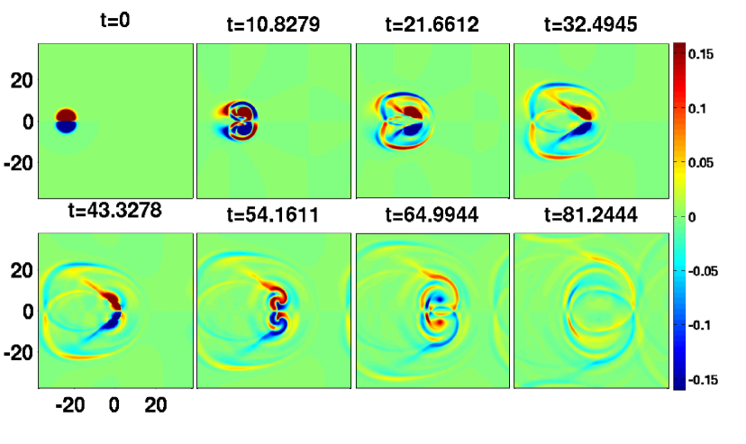
Figure 1: Evolution of sub - luminar dipole in time for visco-elastic fluid of ${\Omega_{0}}$=3.5 with the coupling parameters ${\eta}=5,{\tau_{m}}=20$.

In the other two cases, however, the dipole structure continues to maintain its identity. The wave emission in these cases (because of the super-luminar velocity of dipole) remains confined to a conical spatial regime at the tail. The radiation merely separates the tail region of the dipole somewhat.

In Fig. 2, we show the dipole evolution with more strength i.e. larger velocity amplitude. In this case we restrict speed of dipole not too larger that it leaves behind wake structures. It can be observed that there is wake type structure formation.

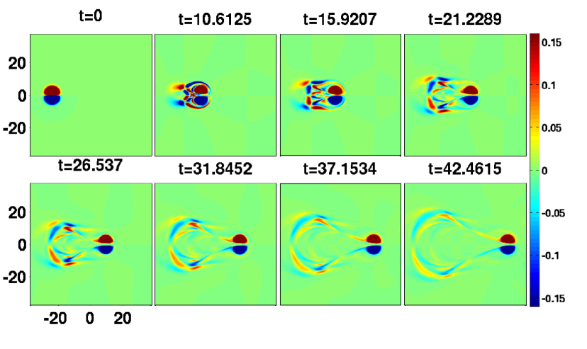
Figure 2: Evolution of super - luminar dipole in time for visco-elastic fluid of ${\Omega_{0}}$=5 with the coupling parameters ${\eta}=5,{\tau_{m}}=20$.

In Fig. 3, we consider the case of dipole moving with more strength than both former cases. The dipole get out of the cage of wake structures.

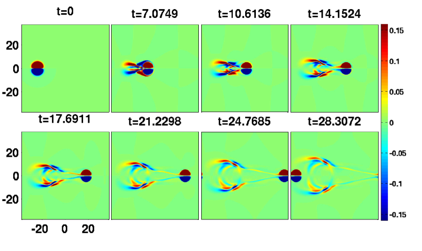
Figure 3: Evolution of super - luminar dipole in time for visco-elastic fluid of ${\Omega_{0}}$=7.5 with the coupling parameters ${\eta}=5,{\tau_{m}}=20$.

Figure 4: Position of maximum of dipole amplitude at different time steps along axial direction with parameter values (a) $\Omega_{0}$=3.5 $(\blacksquare$); $v_{dip}=0.4{<}v_{p}$ corresponds to sub - luminar dipole, (b) $\Omega_{0}$=5 ($\color[rgb]{0,0,0}{\bullet}$); $v_{dip}=1.14{>}v_{p}$ corresponds to super - luminar dipole, and (c) $\Omega_{0}$=7.5 $(\color[rgb]{0,0,0}\bigstar$); $v_{dip}=2.29{>}v_{p}$ is also corresponds to super - luminar dipole, where $v_{dip}$ is the corresponding axial velocity of dipole related to $\Omega_{0}$ and blue line is linear fitted curve.

With increasing speed of the dipole the cone angle between which the TSW radiation is confined is observed to reduce.

IV.2 Head on collision between dipoles

When two oppositely propagating dipoles collide with each other, it is well known in the context of hydrodynamics, that the their lobes exchange partners and form new dipolar structure which propagates orthogonal to the initial propagation direction. This can be observed from the Fig. 5. We consider the two dipoles whose vorticity profile is given by, ${\xi_{0}(x,y,t_{0})}={\xi_{01}(x,y,t_{0})}+{\xi_{02}(x,y,t_{0})}$. Here, right side dipolar vorticity is ${\xi_{01}(x,y,t_{0})}={\Omega_{01}}(y-y_{c1})exp\left(-\left({\left(x-x_{c1}\right)^{2}+(y-y_{c1})^{2}}\right)/{a^{2}_{c1}}\right)$ and left side dipolar vorticity is ${\xi_{02}(x,y,t_{0})}={\Omega_{02}}(y-y_{c2})exp\left(-\left({\left(x-x_{c2}\right)^{2}+(y-y_{c2})^{2}}\right)/{a^{2}_{c2}}\right)$ with parameters ${a_{c1}}$=${a_{c2}}$=2.5, ${x_{c1}}=-24$, ${y_{c1}}$=0, ${x_{c2}}=24$, ${y_{c2}}$=0 and ${\Omega_{01}}$=${\Omega_{02}}$ for equal strength dipoles and different values have been taken for different cases. In cases of disparate strength dipoles ${\Omega_{01}}\neq{\Omega_{02}}$.

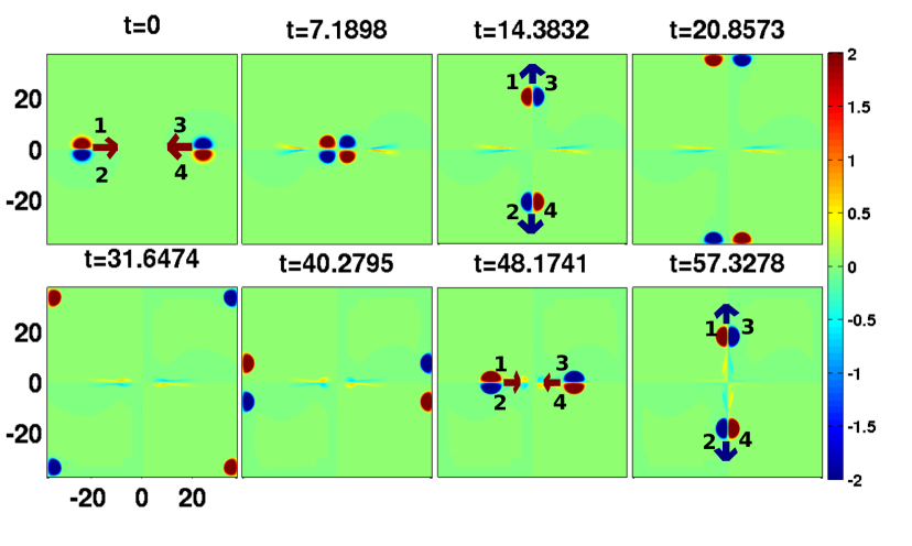
Figure 5: Dipole-dipole head to head collision for hydrodynamic fluid with ${\Omega_{01}}$=${\Omega_{02}}$=7.5.

Similar effect is observed in the context of collision in i-GHD system. We again consider the two cases of collision amidst sub and super - luminar pairs of dipoles in Fig. 6 and Figs. 7,  8 respectively.

In the former case the radiation engulfs the system. The dipoles slow down considerably as they move towards each other. This happens due to the preceding waves from each structure that inhibits their propagation forward. They almost come to a standstill before they exchange partners and then move in the orthogonal direction. This can be observed from the Fig. 6. The identity of the dipolar lobes is ultimately completely lost due to the interaction with the emitted shear waves.

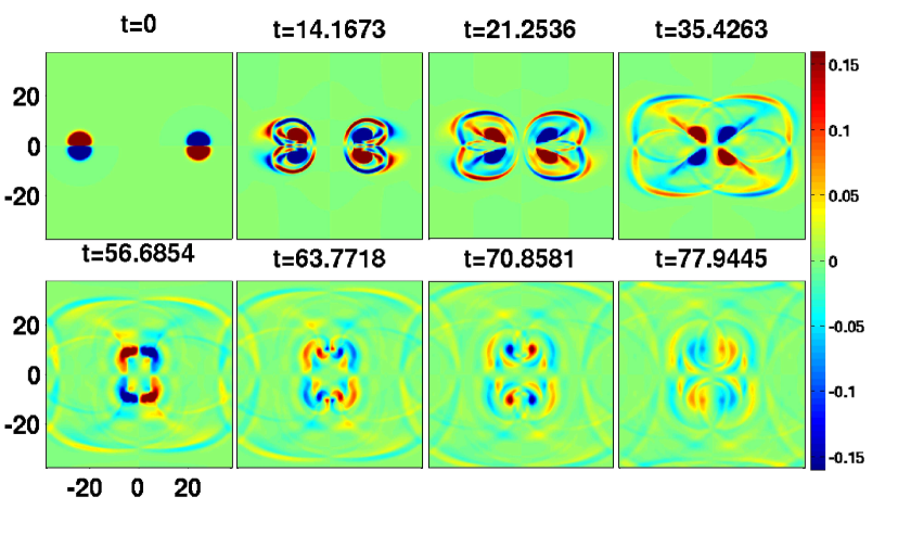
Figure 6: Head to head collision between two equal strength sub - luminar dipoles for visco-elastic fluid of ${\Omega_{01}}$=${\Omega_{02}}$=3.5 with the coupling parameters ${\eta}=5,{\tau_{m}}=20$.

In the second case the dipoles exchange partners and move ahead in the orthogonal direction leaving the radiation behind.

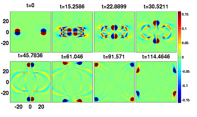
Figure 7: Head to head collision between two equal strength super - luminar dipoles for visco-elastic fluid of ${\Omega_{01}}$=${\Omega_{02}}$=5 with the coupling parameters ${\eta}=5,{\tau_{m}}=20$.

In Fig. 8, we consider the case of dipoles approaching toward each other with more strength than the former cases. The damage in this case to the lobes is very weak and the dipoles retain their identity.

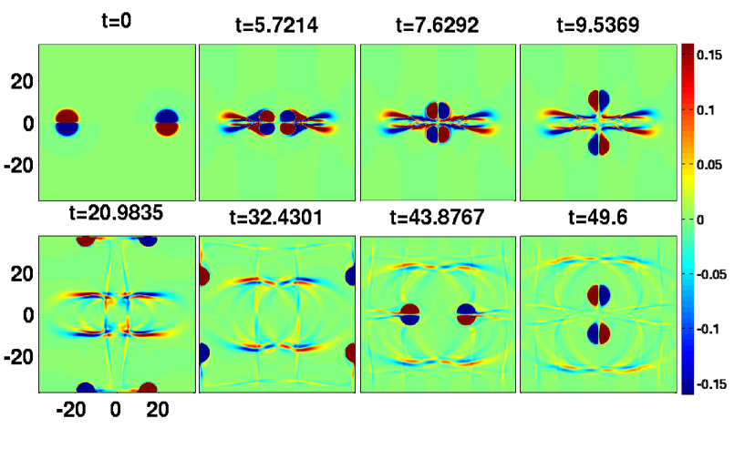
Figure 8: Head to head collision between two equal strength super - luminar dipoles for visco-elastic fluid each of ${\Omega_{01}}$=${\Omega_{02}}$=10 with the coupling parameters ${\eta}=5,{\tau_{m}}=20$.

Collisional interactions of disparate strength dipoles have also been studied. In Fig. 9, we consider two disparate strength dipoles. The sub - luminar dipole on left has ${\Omega_{01}}$= 3.5 and the super - luminar dipole on the right has ${\Omega_{02}}$=10. As opposed to the normal case where the dipoles of equal strength propagate in the direction normal to the direction of propagation before collision, for the present case as evident from Fig. 9, the the super - luminar dipole pierces into the lobes of sub - luminar dipole. It can be clearly seen, after the accomplishment of this crossing process, the lobes of sub - luminar dipole again come close to each other and start propagating like an independent dipole. It is interesting to note that there is no exchange of lobes between dipoles. Both these dipoles (sub and super) propagate in the same direction as before collision. As the time progresses these dipoles interact with the wake type structures (left behind by them) and sub - luminar dipole losses its identity earlier than super - luminar dipole.

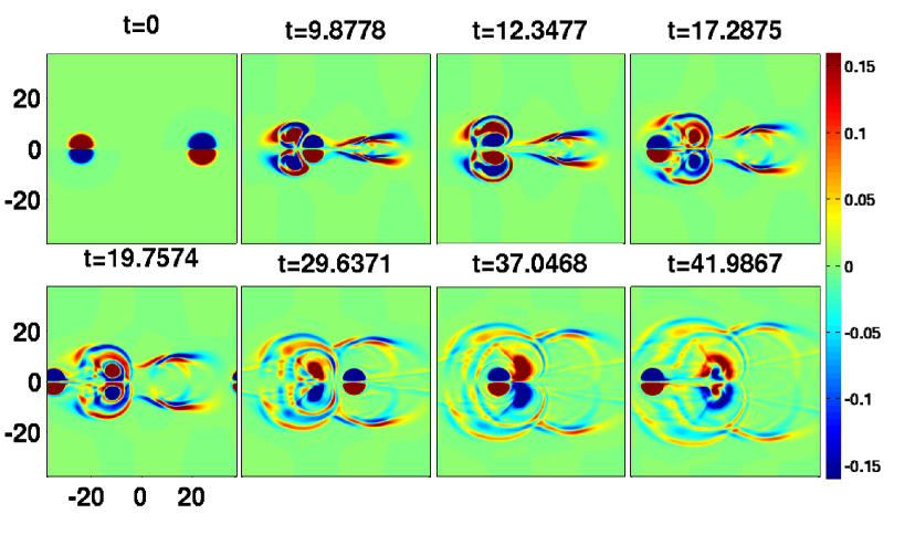
Figure 9: Head to head collision between two disparate strength dipoles, sub - luminar dipole (left) of ${\Omega_{01}}$= 3.5 and super - luminar dipole (right) of ${\Omega_{02}}$=10 with the coupling parameters ${\eta}=5,{\tau_{m}}=20$.

In Fig. 10, we consider two super - luminar disparate strength dipoles, of ${\Omega_{01}}$=7.5 (left) and ${\Omega_{02}}$=10 (right). It is observed that, here after exchanging lobes, these new dipole changes its trajectory and along with the axial motion the weaker lobe rotates around the stronger lobe. With this rotation, new dipoles of unequal lobes strength approaches each other and collide again. The exchange of lobes takes place once again and the newly formed dipoles (with same lobes as before collision process) starts propagating in the same direction just as before collision. This collisional process repeats again and again due to periodic conditions and dipoles also experience the interaction with wake left behind by them.

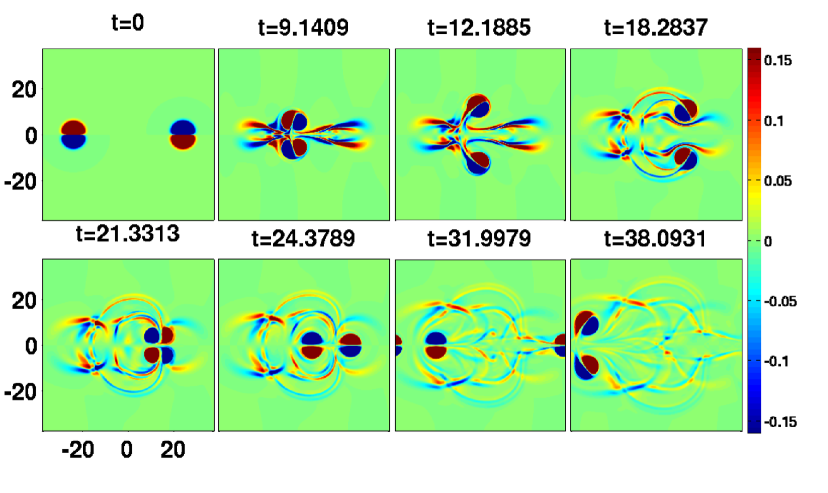
Figure 10: Head to head collision between two disparate strength super - luminar dipoles of ${\Omega_{01}}$= 7.5 (left) and ${\Omega_{02}}$= 10 (right) with the coupling parameters ${\eta}=5,{\tau_{m}}=20$.

All these interactions have shown generation of various complicated radiation and convection patters. We would now take a up a few complex cases and study the accuracy with which the Poynting like conservation theorem is satisfied.

V Numerical verification of Poynting like Equation for i-GHD

We now study the role of different transport processes in the integral equation Eq. (14) on the evolution of $W$ in the context of monopole and dipole evolution.

V.1 For Monopole evolution

We investigated the emission of transverse shear waves from the rotating smooth vorticity profile in strongly coupled dusty plasma medium Dharodi_2014 . In this case the vorticity smooth profile is given by, ${\xi_{0}(x,y,t_{0})}={\Omega_{0}}exp\left(-\left({\left(x-x_{c}\right)^{2}+(y-y_{c})^{2}}\right)/{a^{2}_{c}}\right)$. The numerical simulation has been carried out for ${a_{c}}$=0.5, ${\Omega_{0}}=8$ and ${x_{c}}={y_{c}}$=0. We found that phase velocity $v_{p}$ of such waves is proportional to the coupling strength of the medium. In Fig. 11 the evolution of a circular vorticity patch in the strong coupling limit with parameters (${\eta}=2.5;{\tau_{m}}=20$) for GHD system has been shown. A red circle with a radius of 0.6$\pi$ has been drawn in the plots. Initially all the action is within this circular boundary. However, as time progresses the waves are emitted which cross this boundary. We investigate the validity of the integral Eq. (14) within this boundary. Our simulation region is a square box of length $2\pi$ units with periodic conditions. The periodic condition ensures that the waves would not only propagate out of the circular demarcated region but would also enter it subsequently from the other side due to the periodicity of the square box. In fact the evidence is clear from the subplots in the second row of the Fig. 11.

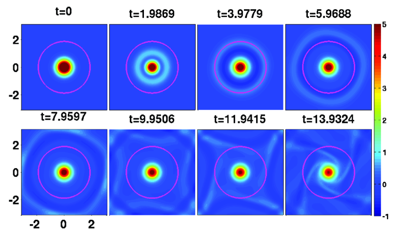
Figure 11: Evolution of smooth circular vorticity profile in time for visco-elastic fluid with the parameters ${\eta}=2.5,{\tau_{m}}=20$ and a circular local volume element (red circumference) over which calculated the different transport quantities.

The change in the magnitude of $W$ within the circular region regime with time is shown in subplot (a) of Fig. 12. We observe a steady decay in magnitude of $W$. It is clear from the plot that the rate of decay of $W$ is not a constant. Thus, the sum of contribution of various terms in Eq. (14) which defines the evolution of $W$ changes with time. The subplot Fig. 12 (b) is $dW/dt$ the slope of $W$ shown in Fig. 12 (a). The evolution of various terms has been shown in the subplots of Fig. 13.

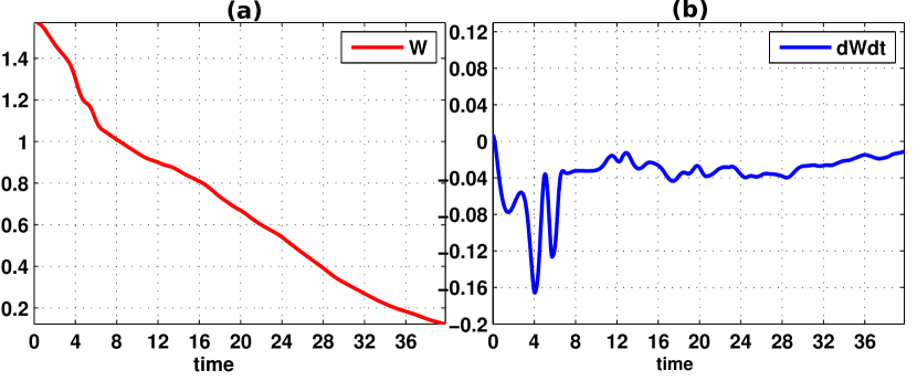
Figure 12: The subplot (a) the conserve quantity $W$ within our considered regime with time and the subplot (b) is the slope of $W$

The subplot (Fig. 13 (a)) represents the change in $W$ by wave emission. It is positive when the waves leave the region and negative when they enter the region. The comparison of subplot (Fig. 13 (a)) with Fig. 11, one can clearly say that the positive peak in this subplot corresponds to the time when the transverse shear waves pulse leaves the circular patch. Similarly, the negative peak here denotes the time when the waves enter the region after re-entering the simulation box from the other end due to the periodic boundary condition. Since, the monopolar vortex remains stationary and merely rotates about its axis so there is no convection of the fluid across the region. Thus, the subplot (Fig. 13 (b)) shows no contribution. The role of dissipating term is shown in subplot of Fig. 13 (c), which is also observed to be finite.

It should be noted that while the contribution from the Poynting flux of wave and convective term can either decrease or increase $W$, the last dissipative terms is always positive and would only cause $W$ to decay.

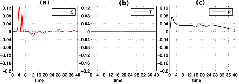
Figure 13: The contribution of each quantity i.e. (a) S, (b) T and (c) $P_{d}$

In Figure 14 we plot $dW/dt$($\color[rgb]{0,0,1}{-}$) and the sum of all the three terms (S+T+P) ($\color[rgb]{1,0,0}{-}$) separately. It can be seen that the two plots are the an accurate mirror image of each other proving that their sum is exactly zero as expected from Eq. (14).

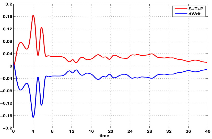
Figure 14: Time derivative of conserved quantity $W$ ($\color[rgb]{0,0,1}{-}$) is the mirror image to the total sum (S+T+P) of all remaining quantities ($\color[rgb]{1,0,0}{-}$) during the run time

V.2 For Dipole evolution

Monopoles being static structures, the contribution due to the convective terms in the equation was negligible as we saw in the previous subsection. We now choose some specific cases of dipoles evolution from earlier section (IV) and study the evolution of the various terms in the Eq. (14) in a circular region of radius $6\pi$. Again, simulation region is a square box of length $24\pi$ units with periodic conditions. The periodic condition ensures that the dipole as well as the emitted waves can enter and leave the region multiple times. The system parameters (system length and circular local volume element) and coupling parameters ($\eta=5$ and $\tau_{m}=20$) are same for all the cases mentioned below. We now show the validity of Eq. (14) for different dipoles with varying strength, $\Omega_{0}$, in the subsequent discussion .

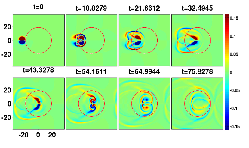
Figure 15: Evolution of dipole with time for visco-elastic fluid of ${\Omega_{0}}$=3.5 with the coupling parameters ${\eta}=5,{\tau_{m}}=20$ and a circular local volume element (red circumference) over which calculated the different transport quantities.

Fig. 15 shows the propagation of the dipolar structures along with the emitted waves. The region inside the red circle is considered for studying the evolution of $W$. The total change in magnitude of conserved quantity $W$ within this region with time is shown in Fig. 16 (a). Since the dipole was placed outside this region initially $W$ was zero to begin with. When the dipole enters this boundary at around time 1.0 $W$ shows a sharp increase. As time progresses the value of $W$ steadily falls owing to the dissipative term (cf. Fig. 17(c)).

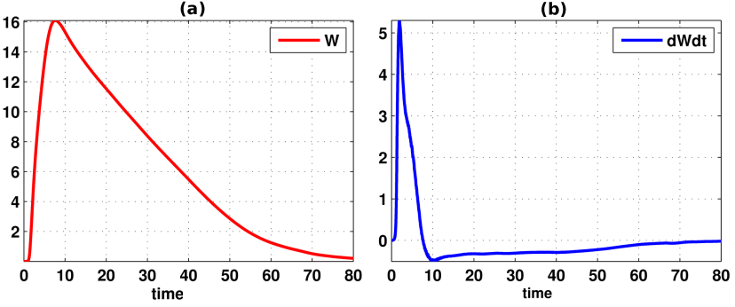
Figure 16: The subplot (a) the conserve quantity $W$ within our considered regime with time and the subplot (b) is the slope of $W$.

When dipole enters this region at around time 1.0, the contribution of transverse and the convection terms can be seen clearly in subplots  17(a),  17(b) respectively.

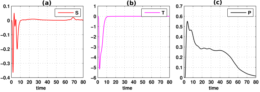
Figure 17: The subplot (a) represents the change in $W$ by wave emission. In case of dipole the major transport process is due to the convection phenomena can be seen in subplot (b). The role of dissipating term is shown in subplot (c), which is observed to be finite.

The conservation equation is pretty accurately satisfied as can be seen from Figure 18 where $dW/dt$ (blue line) and the sum of the three terms has been plotted by red line. They are identical mirror image curves illustrating that the conservation equation $dW/dt+S+P+T=0$ is satisfied with very good precision.

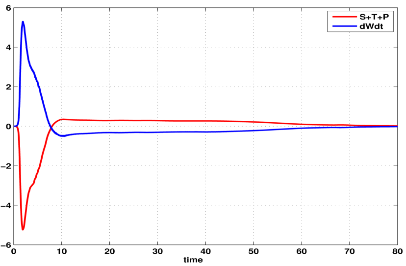
Figure 18: Time derivative of conserved quantity $W$ ($\color[rgb]{0,0,1}{-}$) is the mirror image to the total sum (S+T+P) of all remaining quantities ($\color[rgb]{1,0,0}{-}$) during the run time.

In earlier case (Fig. 15), the dipole was of lesser strength and hence it dissipated inside the circular region considered by us. In Fig. 19, the strength of the dipole is chosen to be sufficiently high so that it can cross the region marked by the red circle over which we are calculating different transport quantities.

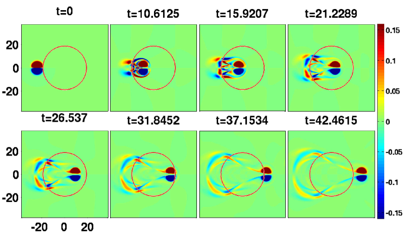
Figure 19: Evolution of dipole with time for visco-elastic fluid of ${\Omega_{0}}$=5.0 with the coupling parameters ${\eta}=5,{\tau_{m}}=20$ and a circular local volume element (red circumference) over which calculated the different transport quantities.

From Fig. 19, it is clear that as the dipole enters and leaves the considered circular region at around time $1$ and $35$ respectively, there is sharp rise and fall in $W$ is also observed as shown in subplot 20 (a). In this time duration the convection term contribute significantly as seen in subplots  21(b) and the contribution of radiation term is smaller as compared to the convection term (cf. subplot 21(a)). However, in the intervening time a steady decrease in $W$ occurs mainly because of the dissipative term shown in subplot 21(c).

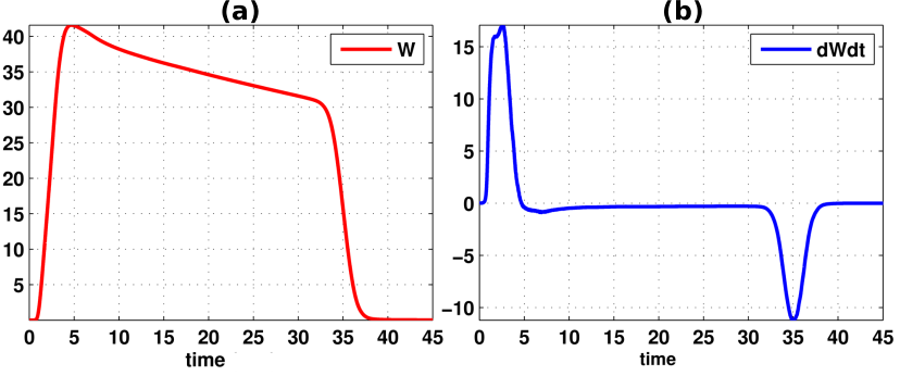
Figure 20: The subplot (a) the conserve quantity $W$ within our considered regime with time and the subplot (b) is the slope of $W$

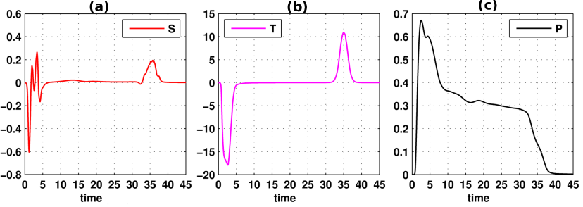
Figure 21: The subplot (a) represents the change in $W$ by wave emission. In this case also the major transport process is due to the convection phenomena can be seen in subplot (b). The role of dissipating term is shown in subplot (c), which is observed to be finite.

From Fig. 22, one observes that $dW/dt$ is the mirror image to the total sum (S+T+P) of all remaining quantities during the run time as observed for earlier cases.

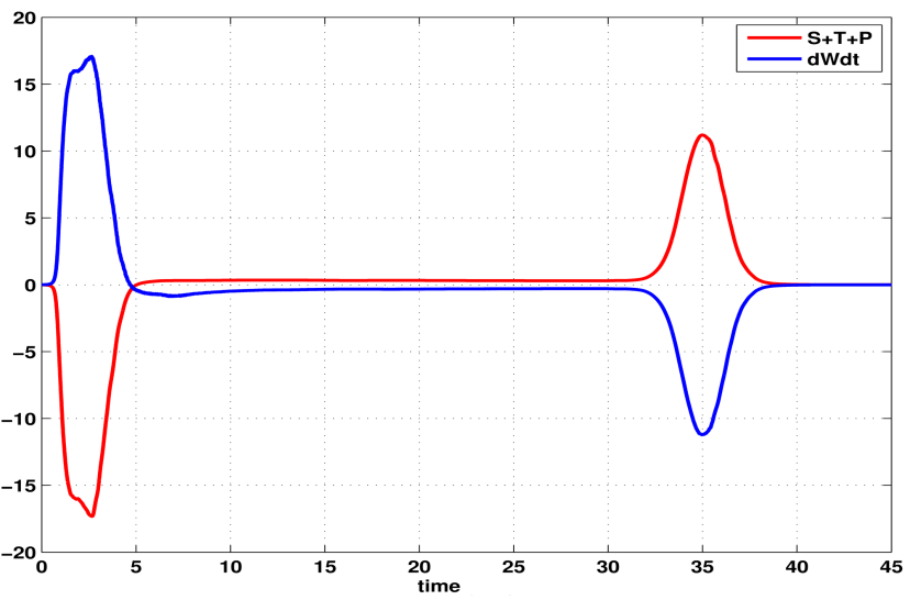
Figure 22: Time derivative of conserved quantity $W$ ($\color[rgb]{0,0,1}{-}$) is the mirror image to the total sum (S+T+P) of all remaining quantities ($\color[rgb]{1,0,0}{-}$) during the run time.

Collision.

In order to confirm the validity of the conservation relation for more complex scenario, we consider the case of two colliding super - luminar disparate strength dipoles of ${\Omega_{01}}$=7.5 (left) and ${\Omega_{02}}$=10 (right) shown in Fig. 23.

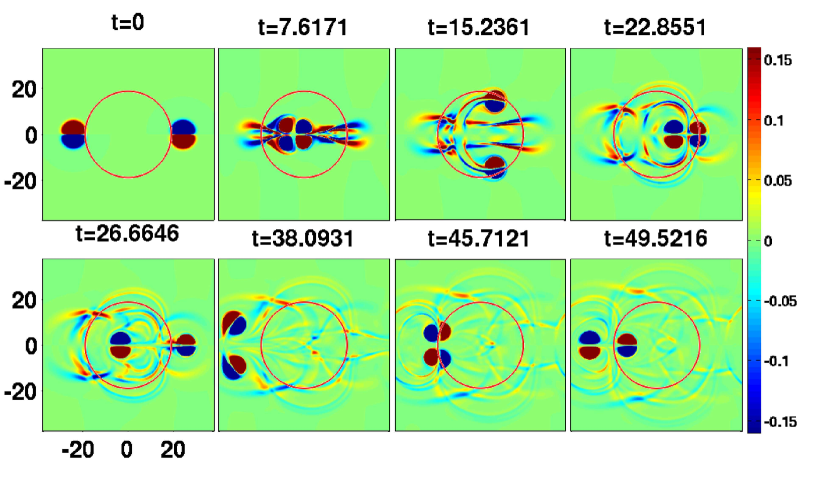
Figure 23: Head to head collision between two disparate strength super - luminar dipoles of ${\Omega_{01}}$= 7.5 (left) and ${\Omega_{02}}$= 10 (right) with the coupling parameters ${\eta}=5,{\tau_{m}}=20$ and a circular local volume element (red circumference) over which calculated the different transport quantities.

The complexity of the motion of dipole is evident in Fig. 23. Here the dipoles exhibits linear/circular motion and collides multiple times inside, outside and along the circumference. This complex evolution of dipoles can be intimately related to the evolution of various terms in the conservation relation. In time duration $5$ to $10$, the dipoles collides axially inside the considered region and then move along the circumference at around time $14$. During this circular motion dipoles share inside and outside vary and finally collide orthogonally to the first collision. This is well reflected in the fluctuation in plot of $W$ shown in Fig. 24(a). Further, in time range ($33$ to $43$) dipoles leave completely this region so $W$ almost becomes zero. Again we observe a sharp increase in $W$ at time around $44$ because of collision between dipoles at the circumference.

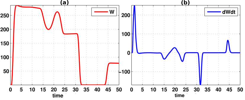
Figure 24: The subplot (a) the conserve quantity $W$ within our considered regime with time and the subplot (b) is the slope of $W$

These events can be corroborated well by observing the contour plot of Fig. 23 and the evolution of the various terms namely, the convective, Poynting and dissipative terms shown in Fig. 25.

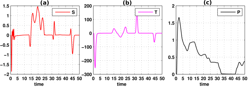
Figure 25: The subplot (a) represents the change in $W$ by wave emission. In this case also the major transport process is due to the convection phenomena can be seen in subplot (b). The role of dissipating term is shown in subplot (c), which is observed to be finite.

Here too the integral condition of Eq. (14) is satisfied identically at all times it can be seen from Fig. 26

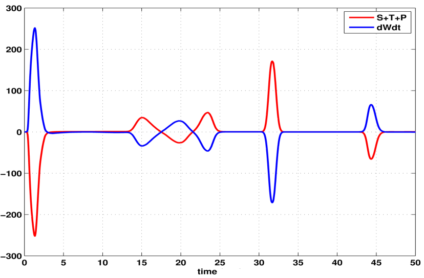
Figure 26: Time derivative of conserved quantity $W$ ($\color[rgb]{0,0,1}{-}$) is the mirror image to the total sum (S+T+P) of all remaining quantities ($\color[rgb]{1,0,0}{-}$) during the run time.

VI Summary and conclusion

The evolution of smooth vorticity profile for a strongly coupled medium by the visco-elastic GHD description have been studied. In contrast to the Newtonian fluid the GHD visco-elastic medium, we have shown numerically the emission of transverse shear waves traveling with phase velocity ${\sqrt{{\eta{}}/{\tau_{m}}}}$ as expected analytically from GHD model. The propagating dipole structures have been studied extensively in both sub/super luminar limits (i.e. when the propagation speed of the dipole is slower/faster than the TSW phase velocity). In the sub - luminar case the dipole remains confined inside the radiation that it emits. Thus the radiation continuously backreacts on the structure which looses its identity soon. On the other hand the radiation emitted by the super - luminar dipole remains confined in a conical wake region of the structure and is unable to distort it. The dipole thus continues to maintain its identity for a much longer duration. Detailed collision studies amidst these structures where also carried out.

A Poynting like conservation theorem was also constructed. The theorem was shown to be satisfied for the GHD set of equations pretty accurately for many complex evolution cases.

References

- [1] C. K. Goertz. Dusty plasmas in the solar system. Reviews of Geophysics, 27(2):271–292, 1989.
- [2] T G Northrop. Dusty plasmas. Physica Scripta, 45(5):475, 1992.
- [3] D A Mendis. Progress in the study of dusty plasmas. Plasma Sources Science and Technology, 11(3A):A219, 2002.
- [4] Padma K Shukla and AA Mamun. Introduction to dusty plasma physics. CRC Press, 2010.
- [5] Laïfa Boufendi and André Bouchoule. Industrial developments of scientific insights in dusty plasmas. Plasma Sources Science and Technology, 11(3A):A211, 2002.
- [6] Alexander Fridman and Lawrence A Kennedy. Plasma physics and engineering. CRC press, 2004.
- [7] Robert L Merlino and John A Goree. Dusty plasmas in the laboratory, industry, and space. Physics Today, 57(7):32–39, 2004.
- [8] Hubertus M. Thomas, Morfill, and E. Gregor. Melting dynamics of a plasma crystal. Nature Publishing Group, 379:806–809, Feb 1996.
- [9] J. H. Chu and Lin I. Direct observation of coulomb crystals and liquids in strongly coupled rf dusty plasmas. Phys. Rev. Lett., 72:4009–4012, Jun 1994.
- [10] H. Thomas, G. E. Morfill, V. Demmel, J. Goree, B. Feuerbacher, and D. Möhlmann. Plasma crystal: Coulomb crystallization in a dusty plasma. Phys. Rev. Lett., 73:652–655, Aug 1994.
- [11] V. E. Fortov, I. T. Iakubov, and A. G. Khrapak. Physics of Strongly Coupled Plasma. Clarendon Press, Oxford, 2006.
- [12] G. Bannasch, T. C. Killian, and T. Pohl. Strongly coupled plasmas via rydberg blockade of cold atoms. Phys. Rev. Lett., 110:253003, Jun 2013.
- [13] H. M. Van Horn. Dense astrophysical plasmas. Science, 252(5004):384–389, 1991.
- [14] P. K. Kaw and A. Sen. Low frequency modes in strongly coupled dusty plasmas. Physics of Plasmas, 5(10), 1998.
- [15] P. K. Kaw. Collective modes in a strongly coupled dusty plasma. Physics of Plasmas, 8(5), 2001.
- [16] D Banerjee, MS Janaki, N Chakrabarti, and M Chaudhuri. Viscosity gradient-driven instability of’shear mode’in a strongly coupled plasma. New Journal of Physics, 12(12):123031, 2010.
- [17] Sanat Kumar Tiwari, Amita Das, Dilip Angom, Bhavesh G. Patel, and Predhiman Kaw. Kelvin-helmholtz instability in a strongly coupled dusty plasma medium. Physics of Plasmas, 19(7):–, 2012.
- [18] Sanat Kumar Tiwari, Vikram Singh Dharodi, Amita Das, Predhiman Kaw, and Abhijit Sen. Kelvin-helmholtz instability in dusty plasma medium: Fluid and particle approach. Journal of Plasma Physics, 2014.
- [19] Sanat Kumar Tiwari, Vikram Singh Dharodi, Amita Das, Bhavesh G Patel, and Predhiman Kaw. Turbulence in strongly coupled dusty plasmas using generalized hydrodynamic description. Physics of Plasmas, 22(2):023710, 2015.
- [20] Samiran Ghosh, Mithil Ranjan Gupta, Nikhil Chakrabarti, and Manis Chaudhuri. Nonlinear wave propagation in a strongly coupled collisional dusty plasma. Phys. Rev. E, 83:066406, Jun 2011.
- [21] M. S. Janaki and N. Chakrabarti. Shear wave vortex solution in a strongly coupled dusty plasma. Physics of Plasmas, 17(5):–, 2010.
- [22] Padma K Shukla and AA Mamun. Dust-acoustic shocks in a strongly coupled dusty plasma. Plasma Science, IEEE Transactions on, 29(2):221–225, 2001.
- [23] J.Frenkel. Kinetic Theory Of Liquids. Dover Publications, 1955.
- [24] MA Berkovsky. Spectrum of low frequency modes in strongly coupled plasmas. Physics Letters A, 166(5):365–368, 1992.
- [25] Setsuo Ichimaru, Hiroshi Iyetomi, and Shigenori Tanaka. Statistical physics of dense plasmas: Thermodynamics, transport coefficients and dynamic correlations. Physics Reports, 149(2-3):91 – 205, 1987.
- [26] J. Pramanik, G. Prasad, A. Sen, and P. K. Kaw. Experimental observations of transverse shear waves in strongly coupled dusty plasmas. Phys. Rev. Lett., 88:175001, Apr 2002.
- [27] H. Ohta and S. Hamaguchi. Wave dispersion relations in yukawa fluids. Phys. Rev. Lett., 84:6026–6029, Jun 2000.
- [28] Vikram Singh Dharodi, Sanat Kumar Tiwari, and Amita Das. Visco-elastic fluid simulations of coherent structures in strongly coupled dusty plasma medium. Physics of Plasmas, 21(7):–, 2014.