Coupled-Channel Model for $\bar{K}N$ Scattering in the Resonant Region

Abstract

We present a unitary multichannel model for $\bar{K}N$ scattering in the resonance region that fulfills unitarity. It has the correct analytical properties for the amplitudes once they are extended to the complex-$s$ plane and the partial waves have the right threshold behavior. To determine the parameters of the model, we have fitted single-energy partial waves up to $J=7/2$ and up to 2.15 GeV of energy in the center-of-mass reference frame obtaining the poles of the $\Lambda^{*}$ and $\Sigma^{*}$ resonances, which are compared to previous analyses. We provide the most comprehensive picture of the $S=-1$ hyperon spectrum to date. Important differences are found between the available analyses making the gathering of further experimental information on $\bar{K}N$ scattering mandatory to make progress in the assessment of the hyperon spectrum.

I Introduction

The comprehensive understanding of strong interactions in the resonance region is an important unresolved issue in particle and nuclear physics. Non-perturbative aspects of QCD related to the question of how quarks and gluons aggregate to build hadrons, can be investigated by analyzing the excited baryon spectrum. Several experiments were devoted in the past to the measurement of $\pi N$ and $\bar{K}N$ scattering as well as meson photoproduction to garner information on the baryon spectrum. The amount of experimental data on hyperon resonances with $S=-1$ ($Y^{*}=\Lambda^{*},\Sigma^{*}$) is not as large as in the case of strangeness zero ($S=0$) nucleon excitations and, as a consequence, the hyperon spectrum is somewhat less understood. For example only recently, following developments in models for $\bar{K}N$ scattering Manley13b ; Kamano14 ; Kamano15 and kaon electroproduction Qiang10 , the Review of Particle Physics (RPP) PDG2014 began to report $Y^{*}$ resonance pole positions. The $\bar{K}N\to\bar{K}N$ reaction amplitudes, besides their importance for studies of the $Y^{*}$ spectrum, play a role in amplitude analysis of more complicated reactions, which include, for example three-body decays, pentaquark searches LHCbpentaquark , or $K\bar{K}$ pair photoproduction ATHOS ; JLAB . For example, recent observation of two pentaquark states in $\Lambda_{b}^{0}\to J/\psi\>K^{-}p$ decay LHCbpentaquark uses a specific model to incorporate $Y^{*}$ resonances in the $K^{-}p$ channel. Studies of systematic uncertainties should, however, involve comparison with other models of $\bar{K}N$ interactions. Real and quasi-real diffractive photoproduction of $K\bar{K}$ pairs can produce the poorly known strangeonia, i.e., mesons containing $s\bar{s}$ pairs that also include exotic mesons with hidden strangeness. To factorize the $K\bar{K}$ photoproduction vertex requires, however, separation of target fragmentation at the amplitude level. Hence, the provision of amplitudes describing, the $\bar{K}N$ interactions in target fragmentation is relevant to future partial-wave analyses of the $\gamma p\to K\bar{K}p$ process. At Jefferson Lab JLAB , both CLAS12 (Hall B) and GluEx (Hall D) experiments will devote part of their effort to study this reaction.

In this article we present a coupled-channel model for $\bar{K}N$ partial waves that incorporates a number of relevant channels, including, for example, $\pi\Sigma$ and $\pi\Lambda$. The approach is based on the $K$-matrix formalism and we pay special attention to the analytical properties of the amplitudes determined by the square-root unitary branch points. This enables continuation of partial waves to the complex $s$-plane and permits a search for amplitude poles (resonances).

The poles of the amplitude that are close to the physical axis in unphysical Riemann sheets determine the behavior of partial waves in the physical region. Identification of baryon resonance poles is one of the goals of meson-baryon amplitude analysis. In recent years, poles of $\bar{K}N$ scattering amplitudes have been reported, initially for the narrow-width $\Lambda(1520)$ Qiang10 , and subsequently from a comprehensive analysis by Zhang et al. Manley13b . Other recent results come from a dynamical coupled-channel model by Kamano et al. Kamano14 ; Kamano15 . Both Manley13b and Kamano15 analyses are in a fair agreement for most of the resonances with a four-star status assigned in the RPP.

This article is organized as follows. In Section II we describe the details of the theoretical model for the partial waves based on the analytical, coupled-channel $K$-matrix representation. In Section III we discuss the fits to the single-energy partial waves, extraction of resonance parameters, and comparison with experimentally measured observables. We also compare with other extractions of $\Lambda^{*}$ and $\Sigma^{*}$ resonance parameters. Finally, in Section IV we present our conclusions and outlook.

II Model

We construct an analytical model that relies on unitarity that enforces square-root singularities at thresholds. Amplitudes are constructed by means of an analytical $K$-matrix representation. Summary of the construction is given below with more details given in Appendix A.

II.1 Observables and Definition of Partial Waves

The differential cross section and polarization for the processes involving $S=-1$ meson-baryon states, which include $\bar{K}N,\pi\Sigma,\ldots\to\bar{K}N,\pi\Sigma,\ldots$ are given by Hoehler1983

$$\frac{d\sigma}{d\Omega}(s,\theta)= \frac{1}{q^{2}}\left[|f(s,\theta)|^{2}+|g(s,\theta)|^{2}\right],$$ (1)

$$P(s,\theta)= \frac{2\>\text{Im}\left[f(s,\theta)\>g^{*}(s,\theta)\right]}{|f(s,\theta)|^{2}+|g(s,\theta)|^{2}},$$ (2)

where $q$ is the magnitude of the relative momentum in the center-of-momentum frame and $\theta$ is the scattering angle. The amplitudes $f(s,\theta)$ and $g(s,\theta)$ correspond to no spin-flip and spin-flip contributions, respectively. These amplitudes are related to the $s$-channel isospin $I=0$ and $I=1$ amplitudes through a general relation

$$f(s,\theta)=\alpha^{0}\>f^{0}_{kj}(s,\theta)+\alpha^{1}\>f^{1}_{kj}(s,\theta),$$ (3)

$$g(s,\theta)=\alpha^{0}\>g^{0}_{kj}(s,\theta)+\alpha^{1}\>g^{1}_{kj}(s,\theta),$$ (4)

where $f^{I}_{kj}(s,\theta)$ and $g^{I}_{kj}(s,\theta)$ are the isospin amplitudes. Here $\alpha^{0}$ and $\alpha^{1}$ are the corresponding Clebsch-Gordan coefficients for isospin zero and one and $kj$ label the initial ($k$) and final ($j$) state, respectively. Specifically, in this work we consider the following cases, for which data are available

$$f^{K^{-}p\to K^{-}p} = \frac{1}{2}f_{\bar{K}N\to\bar{K}N}^{1}+\frac{1}{2}f_{\bar{K}N\to\bar{K}N}^{0},$$ (5)

$$f^{K^{-}p\to\bar{K}^{0}n} = \frac{1}{2}f_{\bar{K}N\to\bar{K}N}^{1}-\frac{1}{2}f_{\bar{K}N\to\bar{K}N}^{0},$$ (6)

$$f^{K^{-}p\to\pi^{-}\Sigma^{+}} = - \frac{1}{2}f_{\bar{K}N\to\pi\Sigma}^{1}-\frac{1}{\sqrt{6}}f_{\bar{K}N\to\pi\Sigma}^{0},$$ (7)

$$f^{K^{-}p\to\pi^{+}\Sigma^{-}} = \frac{1}{2}f_{\bar{K}N\to\pi\Sigma}^{1}-\frac{1}{\sqrt{6}}f_{\bar{K}N\to\pi\Sigma}^{0},$$ (8)

$$f^{K^{-}p\to\pi^{0}\Sigma^{0}} = \frac{1}{\sqrt{6}}f_{\bar{K}N\to\pi\Sigma}^{0},$$ (9)

$$f^{K^{-}p\to\pi^{0}\Lambda} = \frac{1}{\sqrt{2}}f_{\bar{K}N\to\pi\Lambda}^{1},$$ (10)

and similarly for $g(s,\theta)$. Partial-wave expansion of isospin amplitudes is given by

$$f^{I}_{kj}(s,\theta)= \sum_{\ell=0}^{\infty}\left[(\ell+1)R^{I,kj}_{\ell+}(s)+\ell R^{I,kj}_{\ell-}(s)\right]P_{\ell}\left(\theta\right),$$ (11)

$$g^{I}_{kj}(s,\theta)= \sum_{\ell=1}^{\infty}\left[R^{I,kj}_{\ell+}(s)-R^{I,kj}_{\ell-}(s)\right]P^{1}_{\ell}\left(\theta\right),$$ (12)

where $P_{\ell}\left(\theta\right)$ is a Legendre polynomial and $P^{1}_{\ell}\left(\theta\right)=\sin\theta dP_{\ell}\left(\theta\right)/d\cos\theta$. The partial waves $R^{I,kj}_{\ell\tau}(s)$ ($\tau=\pm$) are to be considered as $kj$ elements of the channel-space matrix $R_{\ell}(s)$ as defined below in Eq. (14). In a given meson-baryon channel $\ell$ labels the relative orbital angular momentum and the total angular momentum is given by $J=\ell+\tau/2$. The orbital angular momentum $\ell$ coincides with the orbital angular momentum of the initial $\bar{K}N$ state in $R^{I,kj}_{\ell\tau}(s)$ but it is not necessarily the orbital angular momentum of the other possible states. For example, for the $I=1,\ell=0$ partial wave it is possible to have $\bar{K}\Delta(1232)$ in a $D$ wave state ($L=2$). A complete list of included channels is given in Section III.1. In terms of partial waves, the total cross section is given by

$$\begin{split}\sigma(s)=\frac{4\pi}{q^{2}}\sum_{\ell=0}^{\infty}\left[(\ell+1)|R_{\ell+}(s)|^{2}+\ell\>|R_{\ell-}(s)|^{2}\right],\end{split}$$ (13)

where $R_{\ell\tau}(s)=\alpha^{0}R^{0,kj}_{\ell\tau}(s)+\alpha^{1}R^{1,kj}_{\ell\tau}(s)$.

II.2 Partial-Wave Scattering Matrix

For a given partial wave we write the scattering amplitude as a matrix in the channel-space

$$S_{\ell}=\mathbb{I}+2iR_{\ell}(s)=\mathbb{I}+2i\left[C_{\ell}(s)\right]^{1/2}T_{\ell}(s)\left[C_{\ell}(s)\right]^{1/2},$$ (14)

where $\mathbb{I}$ is the identity matrix, $C_{\ell}(s)$ is a diagonal matrix that accounts for the phase space and $T_{\ell}(s)$ is the analytical partial-wave amplitude matrix. We write $T_{\ell}(s)$ in terms of a $K$ matrix kmatrix to ensure unitarity

$$T_{\ell}(s)=\left[K(s)^{-1}-i\rho(s,\ell)\>\right]^{-1}.$$ (15)

For real $s$, $K(s)$ is a real symmetric matrix and $\rho(s,\ell)$ is a diagonal matrix. To ensure that $\rho(s,\ell)$ is free from kinematical cuts and has only the square-root branch point demanded by unitarity, we write it as a dispersive integral over the phase space matrix $C_{\ell}(s)$, a.k.a. the Chew–Mandelstam representation,

$$i\rho(s,\ell)=\frac{s-s_{k}}{\pi}\int_{s_{k}}^{\infty}\frac{C_{\ell}(s^{\prime})}{s^{\prime}-s}\frac{ds^{\prime}}{s^{\prime}-s_{k}}.$$ (16)

Here $s_{k}$ is the threshold center-of-mass energy squared of the corresponding channel $k$ and we define

$$C_{\ell}(s)=\frac{q_{k}(s)}{q_{0}}\left[\frac{r^{2}q^{2}_{k}(s)}{1+r^{2}q^{2}_{k}(s)}\right]^{\ell}.$$ (17)

The first factor on the r.h.s. of Eq. (17) is related to the breakup momentum near threshold. For a meson-baryon pair with masses $m_{1}$ and $m_{2}$ respectively, $s_{k}=(m_{1}+m_{2})^{2}$ , and

$$\begin{split}q_{k}(s)&=\frac{\sqrt{(s-(m_{1}+m_{2})^{2})(s-(m_{1}-m_{2})^{2})}}{2\sqrt{s}}\\ &\simeq\frac{\sqrt{m_{1}m_{2}}}{(m_{1}+m_{2})}\sqrt{s-s_{k}}.\end{split}$$ (18)

The term in the square bracket ensures the threshold behavior and introduces the effective interaction range parameter, $r=1\>\text{fm}$. Finally, $q_{0}=2\>\text{GeV}$ is a normalization factor for the momentum in the resonance region. Evaluation of the integral in Eq. (16) yields,

$$\begin{split}&i\rho(s,\ell)=\frac{1}{q_{0}r}\left[-\frac{a^{\ell+1/2}_{k}(s-s_{k})^{\ell}\sqrt{s_{k}-s}}{\left[1+a_{k}\>(s-s_{k})\right]^{\ell}}+\frac{\Gamma(\ell+\frac{1}{2})}{\sqrt{\pi}\Gamma(\ell+1)}\right.\\ &\times\left(\left[1+a_{k}(s-s_{k})\right]{{}_{2}F_{1}}\left[1,\ell+\frac{1}{2},-\frac{1}{2},\frac{1}{a_{k}(s_{k}-s)}\right]\right.\\ &\left.\left.-\left[3+2\ell+a_{k}(s-s_{k})\right]{{}_{2}F_{1}}\left[1,\ell+\frac{1}{2},\frac{1}{2},\frac{1}{a_{k}(s_{k}-s)}\right]\right)\right],\end{split}$$ (19)

where $a_{k}=m_{1}m_{2}r^{2}/(m_{1}+m_{2})^{2}$. Notice that Eq. (19) does not require $\ell$ to be integer; hence our amplitudes can be analytically continued both in the $s$ and $\ell$ complex planes Gribov . The physical limit of the amplitudes corresponds to $s+i0$, hence resonances close to the physical region ($s_{p}$ poles in the $T$ matrix) appear at negative values of $\text{Im}s$ when $s$ is continued below the unitary cut of $\rho(s,\ell)$. In Secs. II.3 and II.4 we introduce the building blocks of the $K$ matrix and in Section II.5 we show how these matrices are combined to build the $T$ matrix.

II.3 The Single Pole in the $K$ Matrix

The formalism of Manley et al. Manley serves as a starting point for our model. Given a partial wave that appears in $n_{C}$ channels, it is straightforward to write the elements of the $K$ matrix that may lead to a pole in the amplitude,

$$\left[K_{P}(s)\right]_{kj}=x^{P}_{k}\>\frac{M_{P}}{M_{P}^{2}-s}\>x^{P}_{j}\>.$$ (20)

Here $P$ labels the pole part of $K$. The pole is at a real value of $s=M_{P}^{2}$ and the residue is given in terms of couplings $x^{P}_{k}$ that may be related to partial decay widths. To this end we write,

$$x^{P}_{k}=y^{P}_{k}/\left[|C_{\ell}(M^{2}_{P})|\right]_{kk}\>,$$ (21)

where $\left(y^{P}_{k}\right)^{2}\equiv\Gamma^{P}_{k}$ is to be related to the Breit–Wigner partial-decay width. To see this, we define

$$\Sigma_{P}(s,\ell)=\sum_{k=1}^{n_{C}}\Sigma^{P}_{k}(s,\ell)=\sum_{k=1}^{n_{C}}\left[\rho(s,\ell)\right]_{kk}\left(x^{P}_{k}\right)^{2}.$$ (22)

and

$$\Gamma_{P}(s)=\sum_{k=1}^{n_{C}}\Gamma^{P}_{k}(s)=\sum_{k=1}^{n_{C}}\theta\left(M_{P}^{2}-s_{k}\right)\>\text{Re}\>\Sigma^{P}_{k}(s,\ell),$$ (23)

which at $s=M_{P}^{2}$ reduces to

$$\Gamma_{P}=\sum_{k=1}^{n_{C}}\Gamma^{P}_{k}=\sum_{k=1}^{n_{C}}\left(y^{P}_{k}\right)^{2}\theta\left(M_{P}^{2}-s_{k}\right).$$ (24)

From the relation between $K$ and $T$ matrices in Eq. (15) it follows that the $T$ matrix can be written

$$\left[T_{\ell}(s)\right]_{kj}=x^{P}_{k}\>\mathcal{T}_{P}(s)\>x^{P}_{j}\>,$$ (25)

where

$$\mathcal{T}_{P}(s)=\frac{M_{P}}{M_{P}^{2}-s-iM_{P}\Sigma_{P}(s,\ell)}\>.$$ (26)

Thus $\Gamma^{P}_{k}(s)$ in Eq. (23) is the energy-dependent Breit–Wigner partial width for decay to the $k$-th channel. The $K$-matrix pole mass $M_{P}$ and the couplings $x^{P}_{k}$ are real parameters that will be fitted by comparing the resulting $T$-matrix elements to the data. The resonance pole of the $T$ matrix is given by the solution of equation $M_{P}^{2}-s-iM_{P}\Sigma_{P}(s,\ell)=0$ with $\text{Im}s<0$ on the Riemann sheet analytically connected to the physical region $\text{Im}s\to 0^{+}$ We note that $iM_{P}\Sigma_{P}(s,\ell)$ contributes to both the real and the imaginary parts of the resonance pole.

II.4 Background Contribution to the $K$ Matrix

In addition to resonance poles, which are constrained by the direct channel unitarity, partial-wave amplitudes have dynamical cuts, a.k.a. left hand cuts, which arise when unitarity cuts in the cross-channels are projected onto the direct channel partial waves. In the direct channel physical region, in absence of anomalous thresholds, these non-resonant contributions add up to a smoothly varying background. A simple parameterization of these singularities in the direct channel is to use an expression analogous to that in Eq. (20), i.e. use

$$\left[K_{B}(s)\right]_{kj}=x^{B}_{k}\>\frac{M_{B}}{M_{B}^{2}+s}\>x^{B}_{j}\>.$$ (27)

The label $B$ distinguishes it from the pole contribution to the $K$-matrix. The coefficients $x^{B}_{k}$ are defined by

$$x^{B}_{k}=y^{B}_{k}/\left[C_{\ell}(4\text{GeV}^{2})\right]_{kk}\>,$$ (28)

where $y^{B}_{k}$ is a real number that will be fitted. The parameters $y^{B}_{k}$ are normalized by the phase-space factor as was done for the pole $K_{P}$ matrix parameters, evaluated at an arbitrarily chosen scale of $4$ GeV². If Eq. (27) is used in place of $K_{P}$, then the $T$ matrix becomes

$$\mathcal{T}_{B}(s)=\frac{M_{B}}{M_{B}^{2}+s-iM_{B}\Sigma_{B}(s,\ell)}\>,$$ (29)

where

$$\Sigma_{B}(s,\ell)=\sum_{k=1}^{n_{C}}\Sigma^{B}_{k}(s,\ell)=\sum_{k=1}^{n_{C}}\left[\rho(s,\ell)\right]_{kk}\left(x^{B}_{k}\right)^{2}.$$ (30)

It follows that Eq. (29) has a pole on the real axis at a negative value of $s$. As discussed above this becomes an effective parameterization of non-resonant singularities that originate from exchange processes. Unlike $M_{P}$, the parameter $M_{B}$ in the background parameterization of $K_{B}$ can have any sign (which roughly corresponds to the attractive or repulsive effect of the exchange forces).

II.5 The General Case: Addition of Several $K$ Matrices

In general more than one pole and/or background terms are needed in a given partial wave. Let’s first spell out the result of addition of two $K$ matrices (we drop the $\ell$ index in what follows)

$$\left[K(s)\right]_{kj}=x^{1}_{k}\>K_{1}(s)\>x^{1}_{j}+x^{2}_{k}\>K_{2}(s)\>x^{2}_{j}.$$ (31)

The corresponding $T$ matrix is given by Manley

$$\begin{split}\left[T(s)\right]_{kj}=\frac{1}{\mathcal{D}_{2}(s)}&\left[\>x^{1}_{k}\>c_{11}(s)\>x^{1}_{j}+x^{1}_{k}\>c_{12}(s)\>x^{2}_{j}\right.\\ +&\>\left.x^{2}_{k}\>c_{21}(s)\>x^{1}_{j}+x^{2}_{k}\>c_{22}(s)\>x^{2}_{j}\>\right]\>,\end{split}$$ (32)

where

$$c_{11}(s)= \>\mathcal{T}_{1}(s)\>,$$ (33)

$$c_{22}(s)= \>\mathcal{T}_{2}(s)\>,$$ (34)

$$c_{12}(s)= \>c_{21}(s)=i\epsilon_{12}(s)\mathcal{T}_{1}(s)\mathcal{T}_{2}(s)\>,$$ (35)

$$\mathcal{D}_{2}(s)= \>1+\left(\epsilon_{12}(s)\right)^{2}\mathcal{T}_{1}(s)\mathcal{T}_{2}(s)\>,$$ (36)

and $\mathcal{T}_{1}(s)$ and $\mathcal{T}_{2}(s)$ are given by either Eq. (26) or by Eq. (29) depending on whether $K_{1,2}$ corresponds to the pole or the background parameterization, respectively, and

$$\epsilon_{11}(s)= \sum^{n_{C}}_{k=1}\left[\rho(s,\ell)\right]_{kk}\left(x^{1}_{k}\right)^{2}=\Sigma_{1}(s,\ell)\>,$$ (37)

$$\epsilon_{22}(s)= \sum^{n_{C}}_{k=1}\left[\rho(s,\ell)\right]_{kk}\left(x^{2}_{k}\right)^{2}=\Sigma_{2}(s,\ell)\>,$$ (38)

$$\epsilon_{12}(s)= \epsilon_{21}(s)=\sum^{n_{C}}_{k=1}\left[\rho(s,\ell)\right]_{kk}\>x^{1}_{k}\>x^{2}_{k}\>.$$ (39)

The generalization to several pole/background components

$$\left[K(s)\right]_{kj}=\sum_{a}x^{a}_{k}\>K_{a}(s)\>x^{a}_{j}\>,$$ (40)

yields

$$\left[T(s)\right]_{kj}=\frac{1}{\mathcal{D}(s)}\sum_{a,b}x^{a}_{k}\>c_{ab}(s)\>x^{b}_{j}\>,$$ (41)

where $\mathcal{D}(s)$ and $c_{ab}(s)$ are given by the solution of the system of equations

$$c_{aa}(s)= \mathcal{T}_{a}(s)\left[\mathcal{D}(s)+i\>\sum_{b}(1-\delta_{ab})\>c_{ab}(s)\>\epsilon_{ab}(s)\right],$$ (42)

$$c_{ab}(s)= i\>\mathcal{T}_{a}(s)\left[c_{aa}(s)\>\epsilon_{ab}(s)+\sum_{d}(1-\delta_{ad})\>(1-\delta_{bd})\>c_{ad}(s)\>\epsilon_{bd}(s)\right]\>; \quad a\neq b,$$ (43)

where $c_{ab}(s)=c_{ba}(s)$ and

$$\epsilon_{ab}(s)=\epsilon_{ba}(s)=\sum^{n_{C}}_{k=1}\left[\rho(s,\ell)\right]_{kk}\>x^{a}_{k}\>x^{b}_{k}.$$ (44)

In fits we use up to six pole and background components, $K_{a}$, of the $K$ matrix and up to 13 channels, cf. Table 1. We note that resonance poles in the $T$ matrix are determined by solutions of $\mathcal{D}(s)=0$ in the unphysical Riemann sheets. It encapsulates the difference between $K$-matrix poles and $T$-matrix poles. Explicit solutions of Eqs. (42) and (43) are given in Appendix A.

II.6 Analytic Structure of the $T$ Matrix

The $T$ matrix of the model has the following singularities. It has right-hand cuts due to unitarity whose branch points are placed at corresponding channel thresholds, $s_{k}$. Unitarity gives the discontinuity of the $T$-matrix elements across the right-hand cuts and determines continuation to complex values of $s$ below the real axis where resonance poles are located. There should be no complex poles on the first Riemann sheet, so the equation $\mathcal{D}(s)=0$ should have no complex solutions in the physical, first sheet. The left-hand cuts are represented by poles, on the real axis on the first-sheet below direct channel thresholds. For a single-pole $K$ matrix, as shown in Sec. II.3 the resonance pole of the $T$ matrix is simply related to that of $K$. The background model of $K_{B}$ results in a pole at a real negative value of $s$, approximating the left hand cut. In the general case, $\mathcal{D}(s)$ has a rather complicated structure and the best we can do is to check numerically that the singularities of $T$ are consistent with those described above. In the fits we enforce that any first-sheet pole is far away from the physical region, i.e. we require that it lies at $s<1\>\text{GeV}^{2}$. When several pole and background terms are combined, matching between a certain pole in $K_{P}$ and a resonance pole in $T$ is, in general, lost. Not even the number of resonance poles of $T$ has to be the same as the number of input poles in $K_{P}$ We have taken advantage of this freedom by allowing for various combinations of pole vs. background terms and to assess sensitivity of the data to the presence of certain resonances.

III Results

III.1 Fits to the Single-Energy Partial Waves

Table 1: Summary of the fitted single-energy partial waves. Notation: $n_{P}$: number of pole $K$ matrices; $n_{B}$: number of background $K$ matrices; $n_{C}$: number of channels; $N$: number of fitted single-energy points; $n_{p}$: number of parameters; $\text{dof}=N-n_{p}$: degrees of freedom.

$\ell_{I\>2J}$	$n_{P}$	$n_{B}$	$n_{C}$	$N$	$n_{p}$	dof	$\chi^{2}/N$	$\chi^{2}/\text{dof}$
$S_{01}$	4	2	7	360	43	317	7.64	8.62
$P_{01}$	4	2	6	358	42	316	3.11	3.53
$P_{03}$	2	2	8	508	36	472	1.52	1.64
$D_{03}$	3	1	6	372	28	344	2.25	2.43
$D_{05}$	2	1	5	302	18	284	0.67	0.71
$F_{05}$	2	1	8	460	27	433	1.32	1.41
$F_{07}$	1	1	4	208	10	198	0.11	0.11
$G_{07}$	1	1	6	350	14	336	1.24	1.29
$S_{11}$	4	2	10	546	66	480	8.53	9.70
$P_{11}$	2	3	9	546	50	496	1.68	1.84
$P_{13}$	2	4	11	722	72	650	0.75	0.83
$D_{13}$	1	2	13	814	42	772	0.88	0.93
$D_{15}$	2	1	11	714	36	678	1.09	1.15
$F_{15}$	2	1	12	782	39	743	0.29	0.30
$F_{17}$	1	1	11	704	24	680	0.49	0.51
$G_{17}$	1	0	10	580	11	569	0.10	0.10

The experimental database in the resonance region with $2.19<s<4.70~{}\mbox{GeV}^{2}$, which corresponds to kaon lab momentum of $0.288<p_{\text{lab}}<1.820~{}\mbox{GeV}/c$, Daum1968 ; Andersson1970 ; Albrow1971 ; Conforto1971 ; Adams1975 ; Abe1975 ; Mast1976 ; Alston1978 ; Armenteros1968 ; Armenteros1970 ; Jones1975 ; Griselin1975 ; Conforto1976 ; Prakhov2009 ; Berthon1970a ; Berthon1970b ; Baxter1973 ; London1975 ; Manweiler2008 ; Baldini1988 contains approximately 8000 data points for the $\bar{K}N\to\bar{K}N$ channel ($K^{-}p\to K^{-}p$ and $K^{-}p\to\bar{K}^{0}n$), 4500 for the $\bar{K}N\to\pi\Lambda$ channel ($K^{-}p\to\pi^{0}\Lambda$), and 5000 for the $\bar{K}N\to\pi\Sigma$ channel ($K^{-}p\to\pi^{0}\Sigma^{0}$, $K^{-}p\to\pi^{-}\Sigma^{+}$, and $K^{-}p\to\pi^{+}\Sigma^{-}$). This data set was analyzed in Manley13a and single-energy partial waves were obtained for ($\ell_{I\>2J}$) up to $J=7/2$, namely $S_{01}$, $P_{01}$, $P_{03}$, $D_{03}$, $D_{05}$, $F_{05}$, $F_{07}$, $G_{07}$, $S_{11}$, $P_{11}$, $P_{13}$, $D_{13}$, $D_{15}$, $F_{15}$, $F_{17}$, and $G_{17}$. In Manley13b these partial waves were described in terms of a $K$-matrix model, which in what follows, we refer to as the KSU model. From the model the $\Lambda^{*}$ and $\Sigma^{*}$ spectrum was determined in terms of $T$-matrix poles. Our model is similar to the KSU approach as far as parameterization of the pole $K$ matrix, but differs in construction of the background. Furthermore, in the KSU model unitarity constrains amplitudes only on the real axis, while in the present analysis unitarity is implemented in an analytical way enabling unique continuation of the amplitudes beyond the physical sheet. We compare our results (resonances) to the KSU model in Section III.2.

III.1.1 Channels

We fit the $T$-matrix elements to single-energy partial waves. When evaluating fit uncertainties one should keep in mind that extraction of partial waves from experimental data also carries some model dependence Manley13a ; Manley13b . Consequently, in each partial wave we consider the same set of channels as employed in Manley13a ; Manley13b . The possible initial (final) states correspond to the $k$ ($j$) labels in the $R^{I,kj}_{\ell\tau}(s)$ matrix. All the channels are treated as two-body (meson-baryon) states and are labeled as follows:

• if the state has the same orbital angular momentum ($\ell$) as the partial wave, the channel is identified by the names of the meson and the baryon, e.g. $\bar{K}N$ or $\pi\Sigma$;

• if the baryon has spin $3/2$, as it is the case of $\Sigma(1385)$, $\Delta(1232)$ and $\Lambda(1520)$ (in what follows $\Sigma^{*}$, $\Delta$, and $\Lambda^{*}$ respectively), the orbital angular momentum of the initial state does not correspond to $\ell$ and a subindex $L$ is added denoting the angular momentum of the initial (final) state. For example, in ${\bar{K}}N$ system the $S_{01}$ denotes the isoscalar, $l=0$ partial wave with total spin $J=1/2$. It may couple to $\pi\Sigma^{*}$ with orbital angular momentum $L=2$ ($D$ wave) which we label as $\left[\pi\Sigma^{*}\right]_{D}$;

• if the state contains a spin one $\bar{K}^{*}$ and a nucleon, they can couple to spin $1/2$, which we name $\bar{K}_{1}^{*}N$ or to spin $3/2$, which we name $\bar{K}_{3}^{*}N$. The $\bar{K}_{1}^{*}N$ state has the same orbital angular momentum as the $\bar{K}N$ and the partial wave but the $\bar{K}_{3}^{*}N$ does not, hence we add a $L$ subindex to the last. For example, the $S_{01}$ partial wave has as possible states $\bar{K}_{1}^{*}N$ and $\left[\bar{K}_{3}^{*}N\right]_{D}$.

For every partial wave we include an additional meson-hyperon channel that collectively accounts for any missing inelasticity arising from channels not included explicitly. The kinematical variables for such a dummy channel are chosen arbitrarily as if it were a two-pion $\Lambda$ or $\Sigma$ state labeled as $\pi\pi\Lambda$ for $I=0$ and $\pi\pi\Sigma$ for $I=1$ partial waves. All the channels incorporated in the model have single-energy partial-wave data to fit except for the dummy channels $\pi\pi\Lambda$ and $\pi\pi\Sigma$ and the $\eta\Lambda$ and $\eta\Sigma$ channels in the $S$ waves. The full list of initial (final) states for each partial wave is:

• $\bar{K}N$, $\pi\Sigma$, $\eta\Lambda$, $\bar{K}^{*}_{1}N$, $\left[\bar{K}^{*}_{3}N\right]_{D}$, $\left[\pi\Sigma^{*}\right]_{D}$, $\pi\pi\Lambda$;

• $\bar{K}N$, $\pi\Sigma$, $\bar{K}^{*}_{1}N$, $\left[\bar{K}^{*}_{3}N\right]_{P}$, $\left[\pi\Sigma^{*}\right]_{P}$, $\pi\pi\Lambda$;

• $\bar{K}N$, $\pi\Sigma$, $\bar{K}^{*}_{1}N$, $\left[\bar{K}^{*}_{3}N\right]_{P}$, $\left[\bar{K}^{*}_{3}N\right]_{F}$, $\left[\pi\Sigma^{*}\right]_{P}$, $\left[\pi\Sigma^{*}\right]_{F}$, $\pi\pi\Lambda$;

• $\bar{K}N$, $\pi\Sigma$, $\bar{K}^{*}_{1}N$, $\left[\pi\Sigma^{*}\right]_{S}$, $\left[\pi\Sigma^{*}\right]_{D}$, $\pi\pi\Lambda$;

• $\bar{K}N$, $\pi\Sigma$, $\left[\pi\Sigma^{*}\right]_{D}$, $\left[\pi\Sigma^{*}\right]_{G}$, $\pi\pi\Lambda$;

• $\bar{K}N$, $\pi\Sigma$, $\bar{K}^{*}_{1}N$, $\left[\bar{K}^{*}_{3}N\right]_{P}$, $\left[\bar{K}^{*}_{3}N\right]_{F}$, $\left[\pi\Sigma^{*}\right]_{P}$, $\left[\pi\Sigma^{*}\right]_{F}$, $\pi\pi\Lambda$;

• $\bar{K}N$, $\pi\Sigma$, $\bar{K}^{*}_{1}N$, $\pi\pi\Lambda$;

• $\bar{K}N$, $\pi\Sigma$, $\bar{K}^{*}_{1}N$, $\left[\bar{K}^{*}_{3}N\right]_{D}$, $\left[\bar{K}^{*}_{3}N\right]_{G}$, $\pi\pi\Lambda$;

• $\bar{K}N$, $\pi\Sigma$, $\pi\Lambda$, $\eta\Sigma$, $\bar{K}^{*}_{1}N$, $\left[\bar{K}^{*}_{3}N\right]_{D}$, $\left[\pi\Sigma^{*}\right]_{D}$, $\left[\pi\Lambda^{*}\right]_{P}$, $\left[\bar{K}\Delta\right]_{D}$, $\pi\pi\Sigma$;

• $\bar{K}N$, $\pi\Sigma$, $\pi\Lambda$, $\bar{K}^{*}_{1}N$, $\left[\bar{K}^{*}_{3}N\right]_{P}$, $\left[\pi\Sigma^{*}\right]_{P}$, $\left[\pi\Lambda^{*}\right]_{D}$, $\left[\bar{K}\Delta\right]_{P}$, $\pi\pi\Sigma$;

• $\bar{K}N$, $\pi\Sigma$, $\pi\Lambda$, $\bar{K}^{*}_{1}N$, $\left[\bar{K}^{*}_{3}N\right]_{P}$, $\left[\pi\Sigma^{*}\right]_{P}$, $\left[\pi\Lambda^{*}\right]_{D}$, $\left[\pi\Sigma^{*}\right]_{F}$, $\left[\pi\Lambda^{*}\right]_{S}$, $\left[\bar{K}\Delta\right]_{P}$, $\pi\pi\Sigma$;

• $\bar{K}N$, $\pi\Sigma$, $\pi\Lambda$, $\bar{K}^{*}_{1}N$, $\left[\bar{K}^{*}_{3}N\right]_{S}$, $\left[\bar{K}^{*}_{3}N\right]_{D}$, $\left[\pi\Sigma^{*}\right]_{S}$, $\left[\pi\Sigma^{*}\right]_{D}$, $\left[\pi\Lambda^{*}\right]_{P}$, $\left[\pi\Lambda^{*}\right]_{F}$, $\left[\bar{K}\Delta\right]_{S}$, $\left[\bar{K}\Delta\right]_{D}$, $\pi\pi\Sigma$;

• $\bar{K}N$, $\pi\Sigma$, $\pi\Lambda$, $\bar{K}^{*}_{1}N$, $\left[\bar{K}^{*}_{3}N\right]_{D}$, $\left[\pi\Sigma^{*}\right]_{D}$, $\left[\pi\Sigma^{*}\right]_{G}$, $\left[\pi\Lambda^{*}\right]_{P}$, $\left[\pi\Lambda^{*}\right]_{F}$, $\left[\bar{K}\Delta\right]_{D}$, $\pi\pi\Sigma$;

• $\bar{K}N$, $\pi\Sigma$, $\pi\Lambda$, $\bar{K}^{*}_{1}N$, $\left[\bar{K}^{*}_{3}N\right]_{P}$, $\left[\bar{K}^{*}_{3}N\right]_{F}$, $\left[\pi\Sigma^{*}\right]_{P}$, $\left[\pi\Sigma^{*}\right]_{F}$, $\left[\pi\Lambda^{*}\right]_{D}$, $\left[\pi\Lambda^{*}\right]_{G}$, $\left[\bar{K}\Delta\right]_{P}$, $\pi\pi\Sigma$;

• $\bar{K}N$, $\pi\Sigma$, $\pi\Lambda$, $\bar{K}^{*}_{1}N$, $\left[\bar{K}^{*}_{3}N\right]_{F}$, $\left[\bar{K}^{*}_{3}N\right]_{H}$, $\left[\pi\Sigma^{*}\right]_{F}$, $\left[\pi\Lambda^{*}\right]_{D}$, $\left[\pi\Lambda^{*}\right]_{G}$, $\left[\bar{K}\Delta\right]_{F}$, $\pi\pi\Sigma$;

• $\bar{K}N$, $\pi\Sigma$, $\pi\Lambda$, $\bar{K}^{*}_{1}N$, $\left[\bar{K}^{*}_{3}N\right]_{G}$, $\left[\pi\Lambda^{*}\right]_{F}$, $\left[\pi\Lambda^{*}\right]_{H}$, $\left[\bar{K}\Delta\right]_{D}$, $\left[\bar{K}\Delta\right]_{G}$, $\pi\pi\Sigma$;

The $K\Xi$ channel is not considered in our model because it was not included in the single-energy partial-wave analysis of Manley13a . This channel was not incorporated in Manley13a because the amount of experimental data for that reaction is not enough to perform a reliable partial-wave extraction.

III.1.2 Parameters and Fitting Strategy

The parameters of the model that are fitted to the single-energy partial-wave data are the $K$-matrix parameters, – i.e. $M_{P}$’s for pole and $M_{B}$’s for background, and the pole and background couplings $y_{i}^{P}$’s, $y_{i}^{B}$’s, as given in cf. Eqs. (20) and (27). The summary of the fit results is given in Table 1, where for each partial wave we provide the number of background ($n_{B}$) and pole ($n_{P}$) $K$ terms, the number of channels ($n_{C}$), the number of data points ($N$), the total number of parameters ($n_{p}$), the number of degrees of freedom (dof) and the resulting $\chi^{2}$’s. Due to the large number of parameters, fits have been performed with different strategies and optimization methods until a sufficiently satisfactory solution was obtained. Most of the partial waves, i.e. $P_{13}$, $D_{03}$, $D_{05}$, $D_{13}$, $D_{15}$, $F_{05}$, $F_{07}$, $F_{15}$, $F_{17}$, $G_{07}$ and $G_{17}$, could be fitted using MINUIT MINUIT only, while the other, i.e. $S_{01}$, $S_{11}$, $P_{01}$, $P_{11}$, and $P_{03}$, required more sophisticated methods based on a genetic algorithm genetic combined with MINUIT to increase accuracy as described in genetic . The masses and couplings of the pole $K$ matrices have been guided to yield optimal values for $M_{P}$ and $\Gamma_{P}$ in Eq. (24) penalizing fits that yielded unnatural parameters (such as disproportionate values for the couplings) while the background parameters have been allowed to run freely.

III.1.3 Error Estimation

We have computed the statistical errors of the partial waves parameters and $T$-matrix poles employing the bootstrap technique NumericalRecipes . This calculation is rather straightforward but computationally demanding. It consists of generating, in our case, 50 data sets by randomly sampling the experimental points according to their uncertainties and independently fitting each data sample. The uncertainty for each fitted parameter is given by the standard deviation from the average in 50 fits. For each set of parameters we compute the partial waves, observables and $T$-matrix poles and, again, we estimate the error as the standard deviation.

If the model has problems reproducing a specific partial wave (reflected in large $\chi^{2}/\text{dof}$ values) we perform an additional error estimation by pruning this partial wave. That is, we randomly remove $20\%$ of the data points and fit the remaining $80\%$ of the data. This procedure is repeated 20 times and the standard deviation gives an estimate of the systematic error, these systematic errors have not been propagated to either observables or poles.

Finally, due to the fact that we are fitting single-energy partial waves, our error analysis misses correlations between partial waves as well as systematic uncertainties in the measured differential cross sections and polarization observables. The latter, in those experiments that report them, average to approximately $\pm 10\%$.

III.1.4 Fits

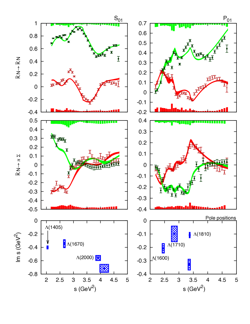
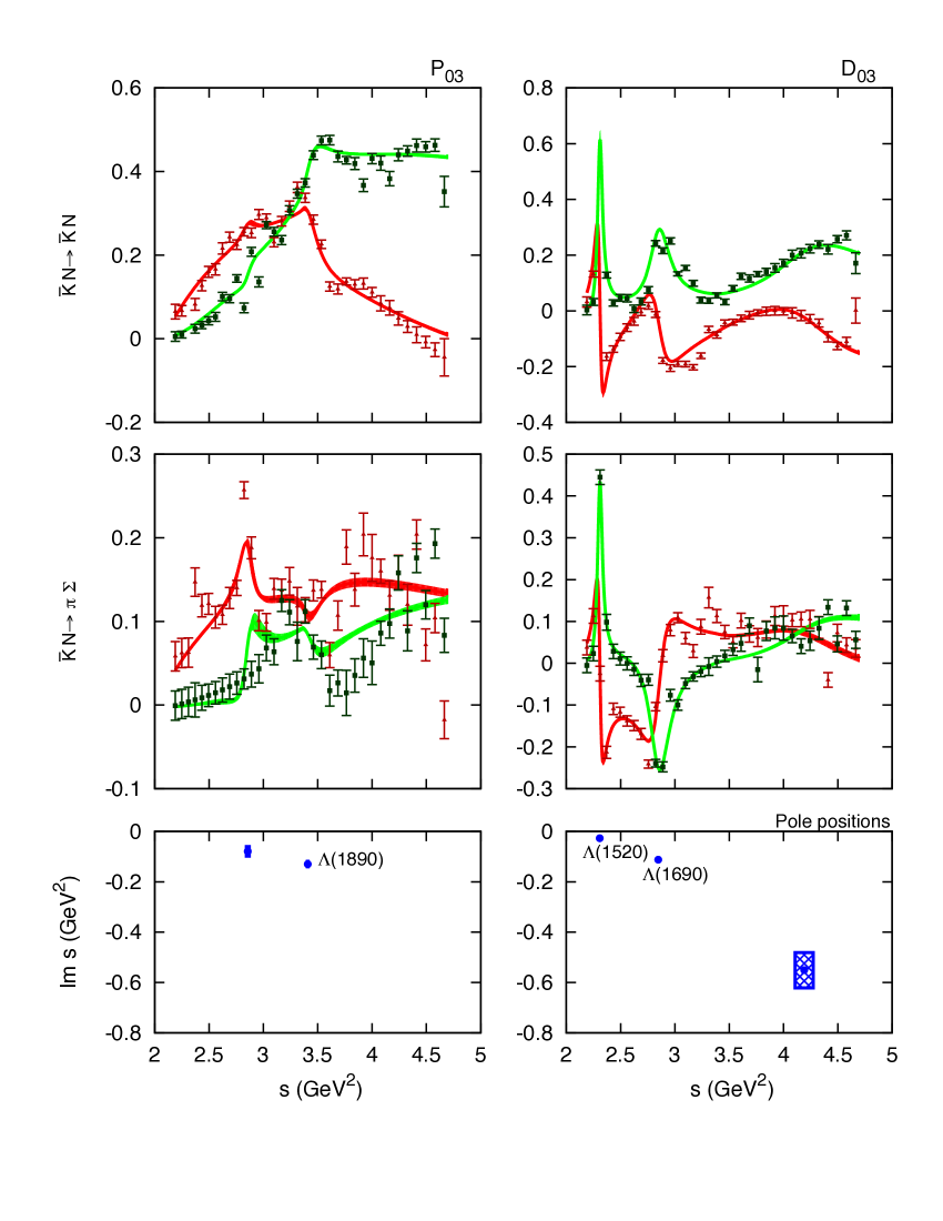
Figure 1: (color online). Partial waves $S_{01}$ (left column), $P_{01}$ (center-left column), $P_{03}$ (center-right column), and $D_{03}$ (right column) together with the $T$-matrix pole positions (last row) compared to the single-energy partial waves from KSU analysis Manley13a for channels $\bar{K}N\to\bar{K}N$ and $\bar{K}N\to\pi\Sigma$ (real part: red triangles; imaginary part: green squares). Red band stands for the real part of the partial wave and green band for the imaginary part of our model. For the $S_{01}$ and $P_{01}$ waves we provide an estimation of the systematic error: bottom-red histogram for the real part of the partial wave and top-green for the imaginary. The resonances (poles of the $T$ matrix) computed are the closest to the physical axis in the corresponding Riemann sheet. One additional pole in the $S_{01}$ partial wave at $2.45-i\>0.47$ GeV² is not shown and believed to be an artifact of the fits (see Sec. III.2.1). Another pole in the $D_{03}$ partial wave at $\left(4.24\pm 0.48\right)-i\left(2.38\pm 0.58\right)$ GeV² is not shown in the bottom-right figure. Error bars for $\Lambda(1520)$, $\Lambda(1690)$ and $\Lambda(1890)$ are smaller than the size of the dots.

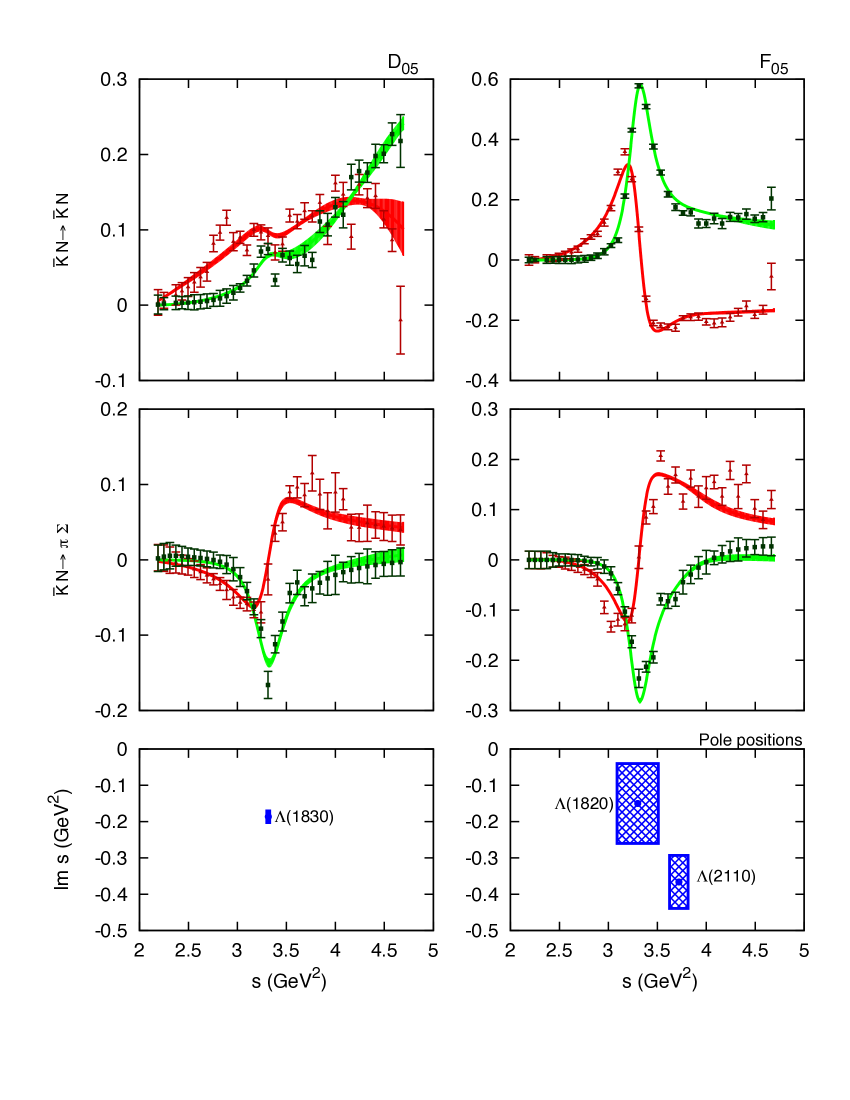
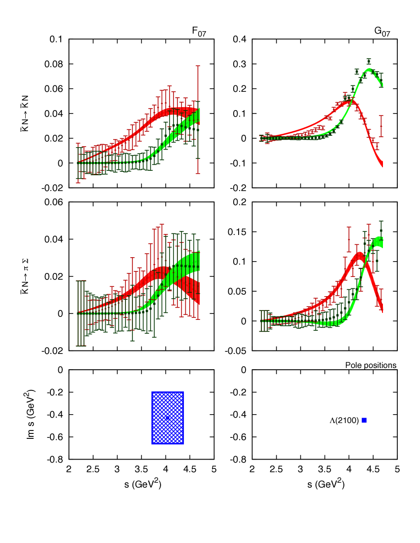
Figure 2: (color online). Same as in Fig. 1 for $D_{05}$ (left column), $F_{05}$ (center-left column), $F_{07}$ (center-right column), and $G_{07}$ (right column) partial waves. An additional pole in the $D_{05}$ partial wave at $\left(4.75\pm 0.19\right)-i\left(1.24\pm 0.41\right)$ GeV² is not shown in the bottom-left figure. The $\Lambda(1820)$ state is found to be highly correlated with a close resonance $\Lambda(2110)$ located at higher energy and deeper in the complex plane.

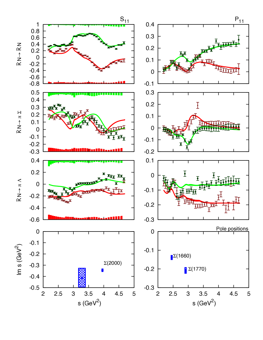
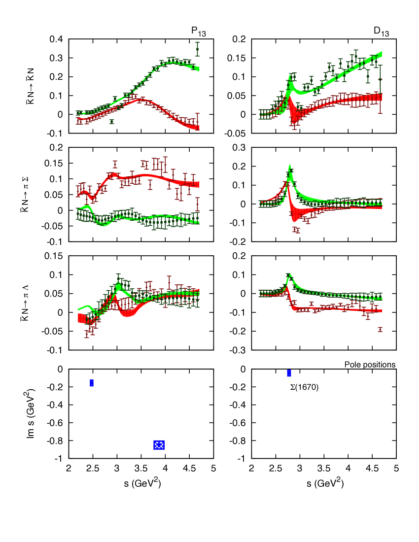
Figure 3: (color online). Partial waves $S_{11}$ (left column), $P_{11}$ (center-left column), $P_{13}$ (center-right column), and $D_{13}$ (right column) together with the pole positions (last row) compared to single-energy partial waves from KSU analysis for channels $\bar{K}N\to\bar{K}N$, $\bar{K}N\to\pi\Sigma$, and $\bar{K}N\to\pi\Lambda$ (real part: red triangles; imaginary part: green squares). Red band stands for the real part of the partial wave and green band for the imaginary part for our model. For the $S_{11}$ wave we provide an estimation of the systematic error: bottom-red histogram for the real part of the partial wave and top-green for the imaginary.

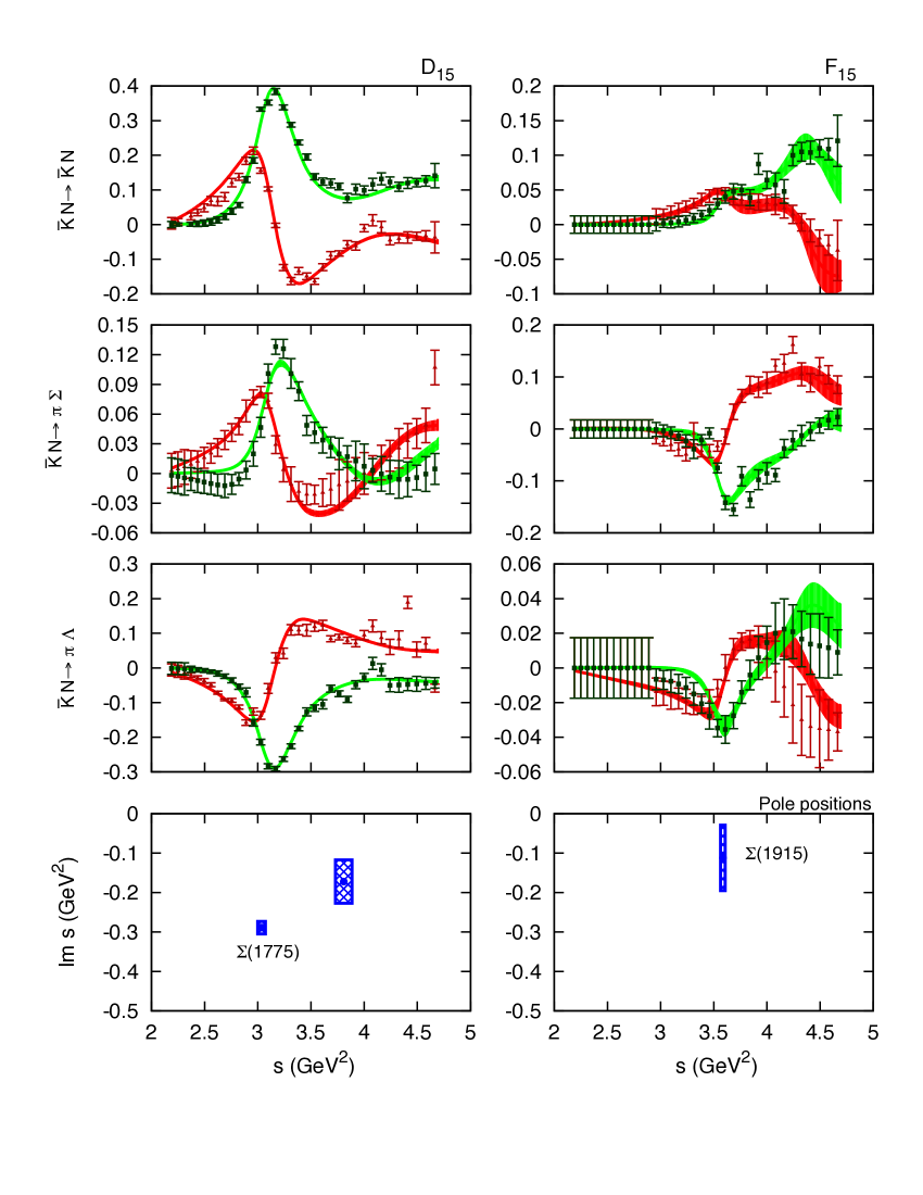
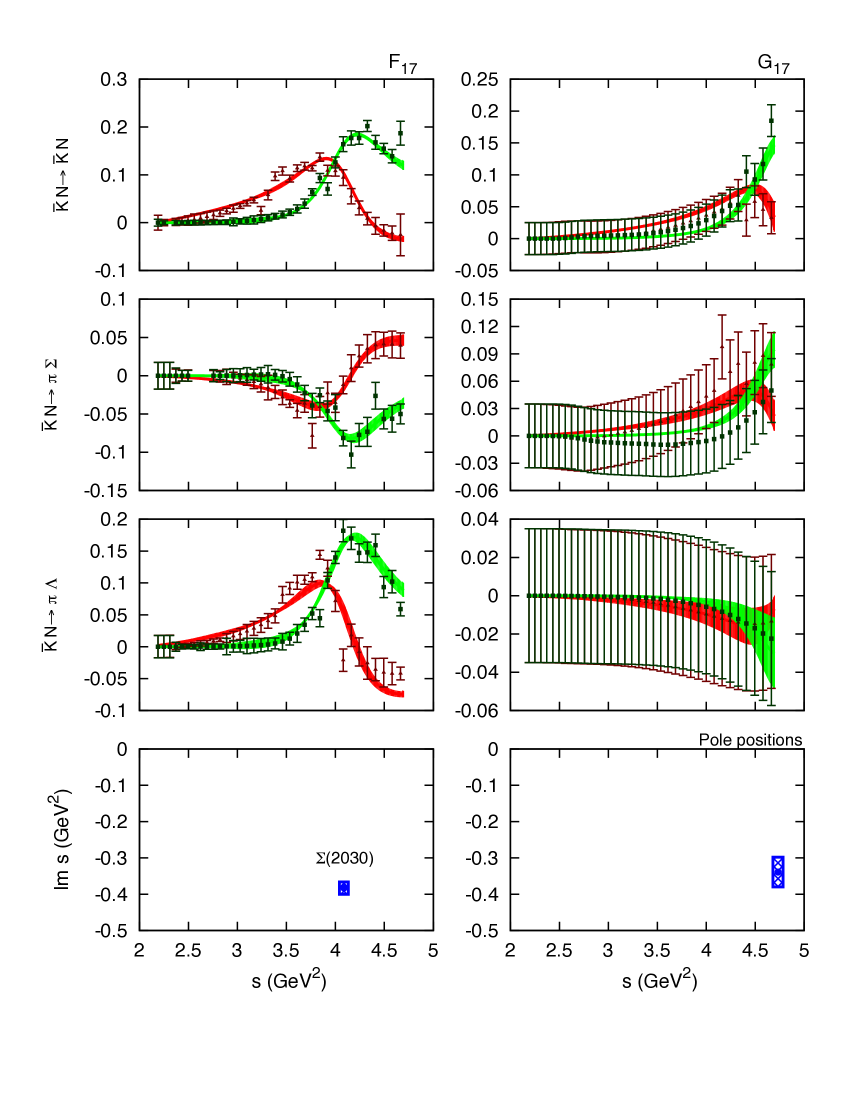
Figure 4: (color online). Same as in Fig. 3 for $D_{15}$ (left column), $F_{15}$ (center-left column), $F_{17}$ (center-right column), and $G_{17}$ (right column) partial waves. An additional pole in the $F_{15}$ partial wave at $\left(4.346\pm 0.026\right)-i\left(0.993\pm 0.018\right)$ GeV² is not shown in the bottom center-left figure.

In Figs. 1–4 we compare our fits to the KSU single-energy partial waves for the channels where there are experimental data available, namely $\bar{K}N\to\pi\Lambda$ for $I=1$ and $\bar{K}N\to\bar{K}N$ and $\bar{K}N\to\pi\Sigma$ for both isospins. The bottom plots in each figure show the position of the $T$-matrix, resonance poles in the Riemann sheet closest to the threshold for the given channel. The values of the pole parameters are given in Tables 2 and 3 and discussed in Section III.2.

The $\chi^{2}/\text{dof}$’s for most of the fits are quite reasonable (see Table 1) and provide a good description of the data as shown in Figs. 1–4. The exceptions are the $S_{01}$, $S_{11}$, $P_{01}$ and $D_{03}$ partial waves.

The $S_{01}$ and $S_{11}$ fits were specially cumbersome. Even with the aid of a genetic algorithm the parameters could get trapped in a local minima and fits needed to be repeated more than 30 times to reach the $\chi^{2}$’s presented in Table 1. It is worth noting that these two partial waves are the most affected by systematic errors and database inconsistencies. For both partial waves we estimate the systematic uncertainty by data pruning and refitting as was described in Section III.1.3. These systematic errors are shown in Figs. 1 and 3 as vertical bars (see figure captions for more details).

The $S_{01}$ for $\bar{K}N\to\bar{K}N$ has a complicated shape. It is rather flat and between 2 and 3 GeV² the imaginary part suddenly drops, which is followed by a bump and another drop. These variations are difficult to reproduce with an analytical parameterization, and results in the large $\chi^{2}/\text{dof}$. Nevertheless, the model seems to describe the general features of both $\bar{K}N\to\bar{K}N$ and $\bar{K}N\to\pi\Sigma$.

One of the main features of the $S_{01}$ partial wave is the appearance of the $\Lambda(1405)$ resonance below the $\bar{K}N$ threshold PDG2014 . This behavior of the $S_{01}$ wave in this mass region is often attributed to existence of two poles, Lambda1405old ; Mai1405 located at $1429^{+8}_{-7}-i\>12^{+2}_{-3}\>\text{MeV}$ and $1325^{+15}_{-15}-i\>90^{+12}_{-18}\>\text{MeV}$ Mai1405 ; Lambda1405 . Our model is built to cover a wide energy range and cannot account for the fine details of the near-threshold effects. For example, the detailed analysis the poles in $\Lambda(1405)$ region required constraints from $\pi\Sigma K^{+}$ photoproduction off the proton Mai1405 . If we do not restrict the fit to obtain a resonance in the region where $\Lambda(1405)$ should appear we obtain $\chi^{2}/\text{dof}\sim 6$ while no resonance poles appear in the $\Lambda(1405)$ region. Hence, we enforce an effective $\Lambda(1405)$ resonance that accounts for both states by penalizing fits that do not generate a pole in this region. The enforcement of this pole results in a more rigid model and a larger $\chi^{2}$.

The $S_{11}$ partial wave has the highest $\chi^{2}/\text{dof}$. Overall, out of the three channels shown in Fig. 3, only the data $\bar{K}N\to\bar{K}N$ can be reasonably well described, except for the real part in the region between 2.5 and 3 GeV². The $\bar{K}N\to\pi\Sigma$ channel of the $S_{11}$ partial wave is reproduced in shape but not in magnitude. The same is true for $\bar{K}N\to\pi\Lambda$. Because of the disagreement with the $S_{11}$ data we cannot accurately reproduce the total cross section data for $K^{-}p\to\pi^{0}\Lambda$ and $s<3$ GeV² (cf. Section III.3).

The difficulties encountered when using a highly constrained analytical model can have several origins. There could be missing resonances or background features in the model, other channels, or there could be inherent problems related to the single-energy extraction. For example, the rapid variation of the partial waves in certain energy regions that the model tries to smear out, may have underestimated uncertainties. The single-energy partial waves were obtained from experimental data in 10 MeV bins, hence rapid variations from one bin to another should be taken with care because a different binning of the data would impact the variation. The uncertainties associated to binning can be assessed by pruning the data and refitting them as was described in Section III.1.3. Finally we note that our channel set overlaps with that of Manley13b which are, for example, not the same as used by Kamano et al. Kamano14 .

When uncertainties and visual inspection are considered, $P_{01}$ and $D_{03}$ (Fig. 1) yield acceptable results. $P_{01}$ shows large uncertainties mostly derived from the difficulty of the imaginary parts to follow the several oscillations of single-energy partial waves in the $2.5-4$ GeV² range for the $\bar{K}N\to\bar{K}N$ and $\bar{K}N\to\pi\Sigma$ channels, that the model tries to average. In the case of the $D_{03}$ partial wave most of the $\chi^{2}/\text{dof}$ is due to the difficulties of the model to follow the rapid variation of the single-energy partial-wave data points in the region of the $\Lambda(1520)$. The change in the partial wave is more rapid than produced by the model. We will return to this discrepancy in $D_{03}$ when comparing to $K^{-}p\to K^{-}p$ observables in Section III.3.

Some of the partial waves show clear signs of over-fitting (very low $\chi^{2}/\text{dof}$), e.g. $F_{07}$, $F_{15}$, $F_{17}$, $G_{17}$. The $F_{07}$ and $G_{17}$ are straightforward to understand, as the data have large uncertainties. The $F_{15}$ and $F_{17}$ cases are different. Because the number of channels for each partial wave is fixed by the single-energy data, the only freedom is in the number of pole and background $K$ matrices. We cannot change the number of parameters one by one until we get the optimal amount of them. For example, the partial wave $F_{17}$ with 11 channels and two $K$ matrices has 24 parameters (two masses and 22 couplings). If we remove one $K$ matrix we drop the number of parameters to 12 (one mass and 11 couplings). With this new model the partial wave still yields a good $\chi^{2}/\text{dof}\sim 0.9$ but the most relevant channels that are straightforwardly connected to experimental data, i.e. $\bar{K}N\to\bar{K}N$, $\bar{K}N\to\pi\Sigma$, and $\bar{K}N\to\pi\Lambda$ are poorly described ($\chi^{2}/\text{dof}\sim 2.5$). Hence, we prefer the model with two $K$ matrices. A similar situation happens with the $F_{15}$ partial wave.

In Section III.2 additional details on the fitting procedure and results are discussed in connection with the $T$-matrix poles determination.

III.2 $T$ Matrix Poles

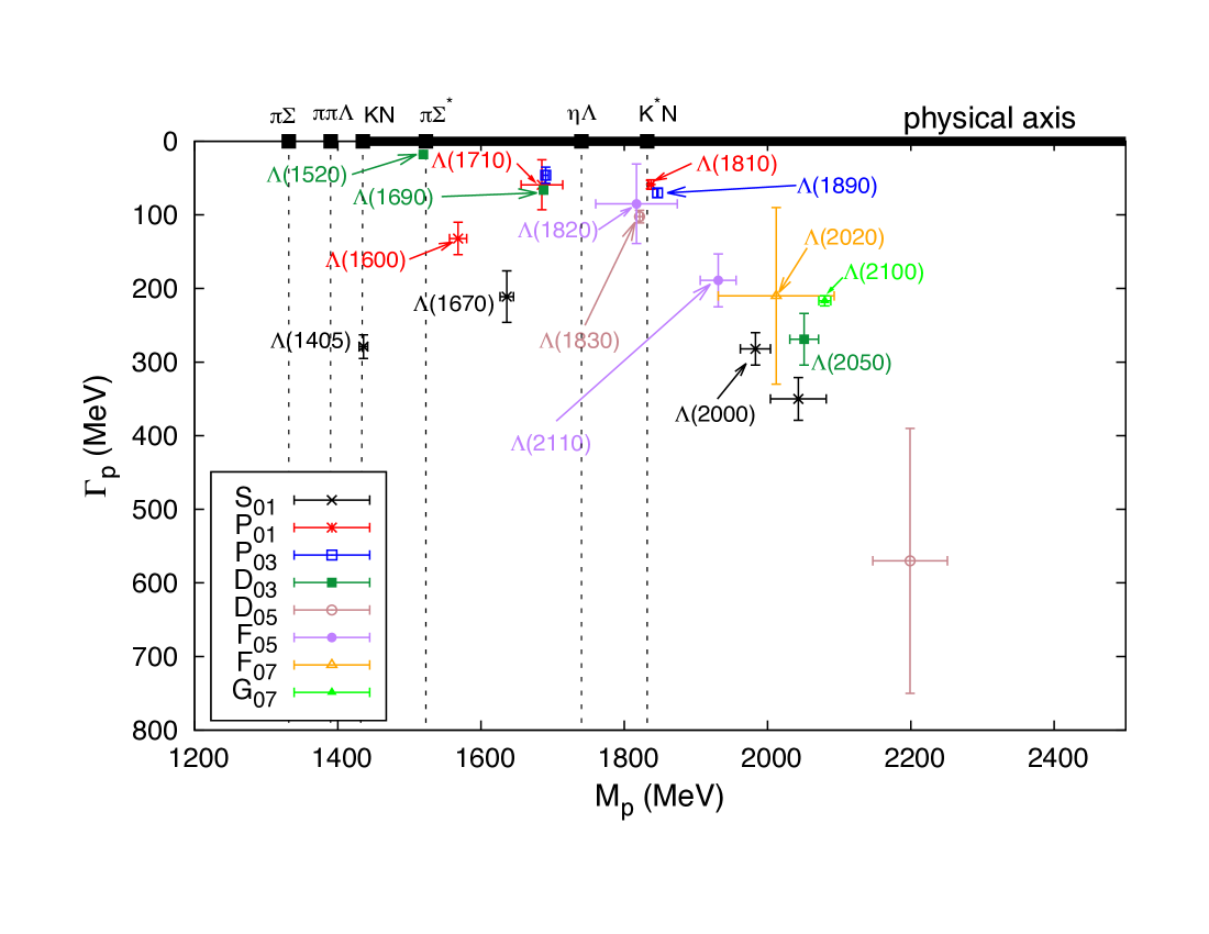
(a)   $\Lambda^{*}$ resonances.

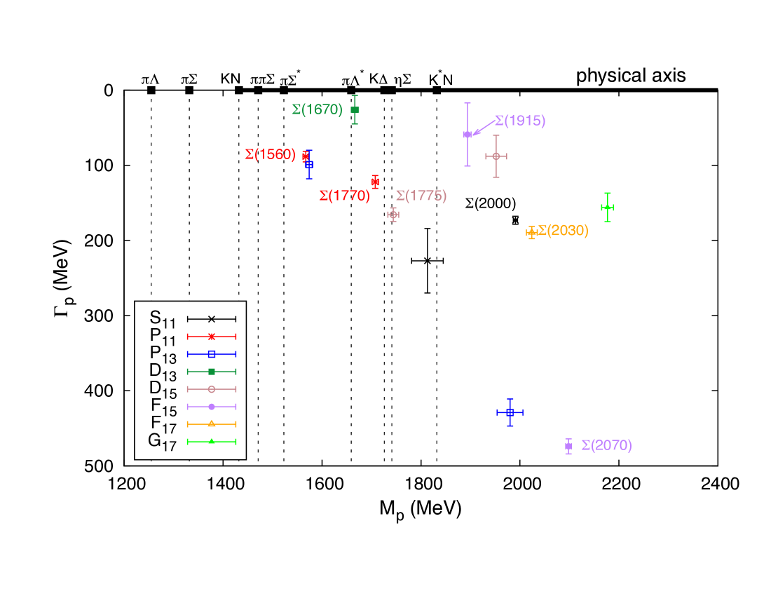
(b)  $\Sigma^{*}$ resonances.

Figure 5: (color online). Poles for $I=0$ (a) and $I=1$ (b) partial waves from Tables 2 and 3 except those with a very large imaginary part and those marked with ‡ (believed to be artifacts of the fits). Poles are computed in the unphysical Riemann sheet where all the available cuts have been crossed (nearest Riemann sheet to the physical amplitude) and their $\ell_{I\>2J}$ quantum numbers are provided. The different thresholds are highlighted as vertical dashed lines and in the physical axis as filled black boxes where $K^{*}$ stands for $K^{*}(892)$, $\Delta$ for $\Delta(1232)$, $\Sigma^{*}$ for $\Sigma(1385)$ and $\Lambda^{*}$ for $\Lambda(1520)$. The last is treated as a stable state and therefore an accessible decay channel in the $I=1$ channels although in the $I=0$ it is a resonance whose properties emerge from our analysis.

The structure found in the partial waves is due to the appearance of poles (resonances) in the $T$ matrix when extended to the unphysical Riemann sheets. These resonances are shown at the bottom in Figs. 1–4. The poles are obtained by computing zeros of $\mathcal{D}(s)=0$ in the nearest unphysical Riemann sheet defined by the crossing of all the available unitarity cuts. $\mathcal{D}(s)$ is defined in Eq. (47). In Tables 2 and 3 we summarized the obtained pole positions, –in the usual notation of masses and widths–, and we compare our results to the KSU model Manley13b and models $A$ and $B$ from Kamano et al. Kamano15 (referred to as KA and KB models in what follows). We also give a possible relation to the resonances listed by the RPP PDG2014 . The poles in the analyses of Kamano et al. are based on a dynamical coupled-channel model described in Kamano14 . Because we use the same single-energy partial waves as the KSU model one would expect a fairly good agreement between the two analyses. There indeed is an agreement for some of the well-established resonances, but several important discrepancies are found in the remaining states, which we discuss in this section. In Fig. 5 we show the resonances from Tables 2 and 3 (except those with very large imaginary part and those believed to be artifacts of the fits) and in Fig. 6 we show the real part of the pole positions on the Chew–Frautschi plot.

Table 2: Summary of $\Lambda^{*}$ pole masses ($M_{p}=\text{Re}\>\sqrt{s_{p}}$) and widths ($\Gamma_{p}=-2\>\text{Im}\>\sqrt{s_{p}}$) in MeV. Our poles are depicted in Fig. 5 unless they have a very large imaginary part or are considered artifacts. In Qiang10 the $\Lambda(1520)$ pole was obtained at ($M_{p}=1518.8$, $\Gamma_{p}=17.2$). Ref. Kamano15 implements two models labeled as KA and KB (see text). $I$ stands for isospin, $\eta$ for naturality, $J$ for total angular momentum, $P$ for parity, and $\ell$ for orbital angular momentum. For baryons, $\eta=+$, natural parity, if $P=(-1)^{J-1/2}$ and $\eta=-$, unnatural parity, if $P=-(-1)^{J-1/2}$. Resonances marked with † are unreliable due to systematics and lack of good-quality $\chi^{2}/\text{dof}$. Resonances marked with ‡ are most likely artifacts of the fits.

	This work		KSU from Manley13b		KA from Kamano15		KB from Kamano15		RPP PDG2014
$I^{\eta}\>J^{P}\>\>\ell$	$M_{p}$	$\Gamma_{p}$	$M_{p}$	$\Gamma_{p}$	$M_{p}$	$\Gamma_{p}$	$M_{p}$	$\Gamma_{p}$	Name	Status
$0^{-}\>\frac{1}{2}^{-}\>S$	$1435.8\pm 5.9^{\dagger}$	$279\pm 16$	1402	49	—	—	—	—	$\Lambda(1405)$	****
	$1573^{\ddagger}$	$300$	—	—	—	—	1512	370	—	—
	$1636.0\pm 9.4^{\dagger}$	$211\pm 35$	1667	26	1669	18	1667	24	$\Lambda(1670)$	****
	—	—	1729	198	—	—	—	—	$\Lambda(1800)$	***
	$1983\pm 21^{\dagger}$	$282\pm 22$	1984	233	—	—	—	—	$\Lambda(2000)$	*
	$2043\pm 39^{\dagger}$	$350\pm 29$	—	—	—	—	—	—	—	—
$0^{+}\>\frac{1}{2}^{+}\>P$	$1568\pm 12$	$132\pm 22$	1572	138	1544	112	1548	164	$\Lambda(1600)$	***
	$1685\pm 29^{\dagger}$	$59\pm 34$	1688	166	—	—	—	—	$\Lambda(1710)$	*
	$1835\pm 10^{\ddagger}$	$180\pm 22$	—	—	—	—	—	—	—	—
	$1837.2\pm 3.4^{\dagger}$	$58.7\pm 6.5$	1780	64	—	—	1841	62	$\Lambda(1810)$	***
	—	—	2135	296	2097	166	—	—	—	—
$0^{-}\>\frac{3}{2}^{+}\>P$	$1690.3\pm 3.8$	$46.4\pm 11.0$	—	—	—	—	1671	10	—	—
	$1846.36\pm 0.81$	$70.0\pm 6.0$	1876	145	1859	112	—	—	$\Lambda(1890)$	****
	—	—	2001	994	—	—	—	—	—	—
$0^{+}\>\frac{3}{2}^{-}\>D$	$1519.33\pm 0.34$	$17.8\pm 1.1$	1518	16	1517	16	1517	16	$\Lambda(1520)$	****
	$1687.40\pm 0.79$	$66.2\pm 2.3$	1689	53	1697	66	1697	74	$\Lambda(1690)$	****
	$2051\pm 20$	$269\pm 35$	1985	447	—	—	—	—	$\Lambda(2050)$	*
	$2133\pm 120^{\ddagger}$	$1110\pm 280$	—	—	—	—	—	—	$\Lambda(2325)$	*
$0^{-}\>\frac{5}{2}^{-}\>D$	$1821.4\pm 4.3$	$102.3\pm 8.6$	1809	109	1766	212	—	—	$\Lambda(1830)$	****
	—	—	1970	350	1899	80	1924	90	—	—
	$2199\pm 52$	$570\pm 180$	—	—	—	—	—	—	—	—
$0^{+}\>\frac{5}{2}^{+}\>F$	$1817\pm 57$	$85\pm 54$	1814	85	1824	78	1821	64	$\Lambda(1820)$	****
	$1931\pm 25$	$189\pm 36$	1970	350	—	—	—	—	$\Lambda(2110)$	***
$0^{-}\>\frac{7}{2}^{+}\>F$	—	—	—	—	1757	146	—	—	—	—
	$2012\pm 81$	$210\pm 120$	1999	146	—	—	2041	238	$\Lambda(2020)$	*
$0^{+}\>\frac{7}{2}^{-}\>G$	$2079.9\pm 8.3$	$216.7\pm 6.8$	2023	239	—	—	—	—	$\Lambda(2100)$	****

Table 3: Summary of $\Sigma^{*}$ pole masses ($M_{p}=\text{Re}\>\sqrt{s_{p}}$) and widths ($\Gamma_{p}=-2\>\text{Im}\>\sqrt{s_{p}}$) in MeV. Our poles are depicted in Fig. 5 unless they have a very large imaginary part. Notation is the same as in Table 2. Resonances marked with † are unreliable due to systematics and lack of good-quality $\chi^{2}/\text{dof}$.

	This work		KSU from Manley13b		KA from Kamano15		KB from Kamano15		RPP PDG2014
$I^{\eta}\>J^{P}\>\>\ell$	$M_{p}$	$\Gamma_{p}$	$M_{p}$	$\Gamma_{p}$	$M_{p}$	$\Gamma_{p}$	$M_{p}$	$\Gamma_{p}$	Name	Status
$1^{-}\>\frac{1}{2}^{-}\>S$	—	—	1501	171	—	—	1551	376	$\Sigma(1620)$	*
	—	—	1708	158	1704	86	—	—	$\Sigma(1750)$	***
	$1813\pm 32^{\dagger}$	$227\pm 43$	—	—	—	—	—	—	—	—
	—	—	1887	187	—	—	—	—	$\Sigma(1900)$	*
	$1990.8\pm 4.3^{\dagger}$	$173.1\pm 5.4$	—	—	—	—	1940	172	$\Sigma(2000)$	*
	—	—	2040	295	—	—	—	—	—	—
$1^{+}\>\frac{1}{2}^{+}\>P$	$1567.3\pm 5.7$	$88.4\pm 7.0$	—	—	1547	184	1457	78	$\Sigma(1560)$	**
	—	—	—	—	—	—	—	—	$\Sigma(1660)$	***
	$1707.7\pm 6.6$	$122.1\pm 8.5$	1693	163	1706	102	—	—	$\Sigma(1770)$	*
	—	—	1776	270	—	—	—	—	$\Sigma(1880)$	**
	—	—	—	—	—	—	2014	140	—	—
$1^{-}\>\frac{3}{2}^{+}\>P$	$1574.1\pm 7.2$	$99\pm 19$	—	—	—	—	—	—	—	—
	—	—	1683	243	—	—	—	—	—	—
	—	—	1874	349	—	—	—	—	—	—
	$1980\pm 26$	$429\pm 18$	—	—	—	—	—	—	—	—
$1^{+}\>\frac{3}{2}^{-}\>D$	—	—	—	—	1607	252	1492	138	$\Sigma(1580)$	*
	$1666.3\pm 7.0$	$26\pm 19$	1674	54	1669	64	1672	66	$\Sigma(1670)$	****
	—	—	—	—	—	—	—	—	$\Sigma(1940)$	***
$1^{-}\>\frac{5}{2}^{-}\>D$	$1744\pm 11$	$165.7\pm 9.0$	1759	118	1767	128	1765	128	$\Sigma(1775)$	****
	$1952\pm 21$	$88\pm 28$	2183	296	—	—	—	—	—	—
$1^{+}\>\frac{5}{2}^{+}\>F$	—	—	—	—	—	—	1695	194	—	—
	$1893.9\pm 7.2$	$59\pm 42$	1897	133	1890	99	—	—	$\Sigma(1915)$	****
	$2098.2\pm 5.8$	$474\pm 10$	2084	319	—	—	—	—	$\Sigma(2070)$	*
$1^{-}\>\frac{7}{2}^{+}\>F$	$2024\pm 11$	$189.5\pm 8.1$	1993	176	2025	130	2014	206	$\Sigma(2030)$	****
$1^{+}\>\frac{7}{2}^{-}\>G$	$2177\pm 12$	$156\pm 19$	2252	290	—	—	—	—	$\Sigma(2100)$	*

As explained in Section II.6, in our model there are no poles on the first Riemann sheet except for those on the real axis below thresholds parameterizing the left-hand cut. These poles, in most of the cases were found to be far away from the physical region. The poles closest to the physical region are found in $F_{05}$ at $-0.45$ GeV², $D_{13}$ at $-0.41$ GeV², $P_{03}$ at $0.08$ GeV², $S_{11}$ at $0.31$ GeV², $S_{01}$ at $0.38$ GeV², and $P_{13}$ at $0.88$ GeV², and they all produce a smooth behavior in the physical region.

The resonance poles are mainly responsible for giving structure to the partial waves on the real axis. Therefore, when the fit is not very good the model tries to smear the structures that it is not able to reproduce. If we take a set of parameters (far from the best-fit parameters but not too far) in a certain partial wave and we do a pole search it is likely that we find fewer resonances than for the best fit. As $\chi^{2}/\text{dof}$ improves, more resonances appear. If we overfit the data, we start to identify as structure some variations in the data that could potentially be identified as a statistical noise instead of genuine resonances. Hence, pole extraction from under-fitted and over-fitted waves has to be treated with care.

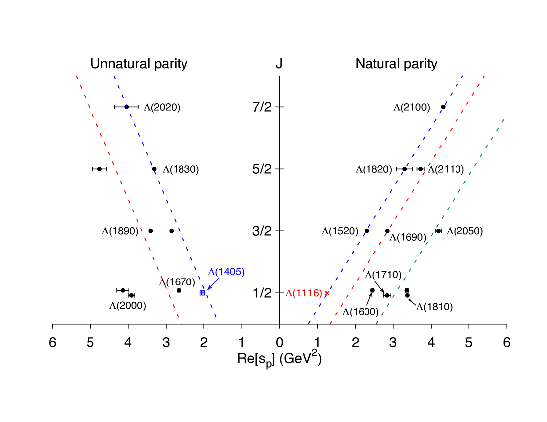
(a)   $\Lambda^{*}$ resonances.

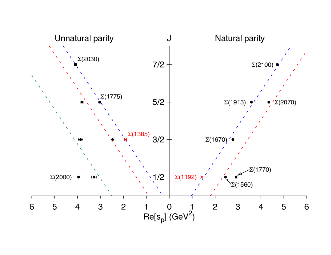
(b)  $\Sigma^{*}$ resonances.

Figure 6: (color online). Chew–Frautschi plot for the $\Lambda^{*}$ (a) and $\Sigma^{*}$ (b) resonances. Poles are displayed according to positive (natural) or negative (unnatural) naturality ($\eta$). Poles colored in red, i.e. $\Lambda(1116)$, $\Sigma(1192)$ and $\Sigma(1385)$, are taken from RPP PDG2014 . The $\Lambda(1405)$ is displayed in blue to highlight that in our approach it is an effective state that mimics two actual resonances (see text). Dashed lines are displayed to guide the eye through the Regge trajectories. Blue lines guide the eye through the parent Regge trajectories while red and green guide through the daughter trajectories.

III.2.1 $\Lambda^{*}$ Resonances

All the $\Lambda^{*}$ resonances obtained are summarized in Table 2 and almost all are displayed in Figs. 5(a) and 6(a) (see respective captions for details). Throughout this section pole masses and widths are reported in MeV unless stated otherwise.

$\mathbf{S_{01}}$ poles. Besides the $\Lambda(1405)$ (which was imposed as explained in Section III.1) we find four resonances in our best fit of the $S_{01}$ partial wave. The first one at $1573-i\>300/2$ is close to the one obtained by model KB at $1512-i\>370/2$ and is not obtained by any other model. We believe it is an artifact of the fit because when we perform the bootstrap to obtain the error bars, it does disappears from most of the fits. Hence, we do not quote an error bar for it in Table 2 and we do not show it in Figs. 1, 5(a), and 6(a). Two of the other poles can be associated with $\Lambda(1670)$ and $\Lambda(2000)$ states in the RPP. The $\Lambda(2000)$ pole agrees with KSU analysis and is not found either by KA or KB. The $\Lambda(1670)$ has a four-star status in the RPP. The mass we obtain is within a reasonable range when compared to the KSU, KA, and KB analyses, although our width is larger with a sizable uncertainty. This pole appears in the energy region where our model does not reproduce properly the abrupt change in the $\bar{K}N\to\pi\Sigma$ channel around 2.8 GeV² (see left column in Fig. 1) so the width we obtain is not very reliable. We also find a higher-energy resonance that no other analysis finds. Further confirmation of its existence is needed. Neither us nor KA nor KB find a pole close to the $1729-i\>198/2$, $\Lambda(1800)$, found in KSU analysis. This pole has a three-star status and, considering the large systematic uncertainties of the $S_{01}$ wave its status might need to be reconsidered in the RPP. Nevertheless, because of the systematic uncertainties and the high $\chi^{2}/\text{dof}$ we cannot make definitive statements on the $S_{01}$ pole locations.

$\mathbf{P_{01}}$ poles. In the $P_{01}$ partial wave we find four resonances. The lowest-lying is at $1568-i132/2$, which corresponds to the three-star $\Lambda(1600)$. All the analysis, KSU, KA, KB and us, agree on the location of this resonance within their uncertainties making it a very well established state. However, when we try to identify which Regge trajectory it belongs to (see Fig. 6(a)) it looks like it does not match the general pattern. This signals that the $\Lambda(1600)$ resonance is of different nature than the other resonances we are finding and that it is not an ordinary three-quark state. The $\Lambda(1710)$ state was first introduced by KSU analysis and we find a pole at similar mass but closer to the real axis. This state needs further confirmation through an independent analysis given that we obtain a smaller width than KSU model and we both fit the same single-energy partial waves. However, our result together with those of KSU and rhohyperon reinforce the hypothesis that there are two poles in the $P_{01}$ partial wave for $\sqrt{s}<1.9$ GeV. In rhohyperon a non-three-quark nature is suggested for both states. We also obtain a pole at $1837.2-i58.7/2$ that can be identified as the $\Lambda(1810)$ state and is in very good agreement with the pole at $1841-i62/2$ obtained by the KB model. The reliability of the $\Lambda(1810)$ pole position can be questioned due to the appearance of a pole at $1835-i\>180/2$ that looks like an artifact linked to the opening of the $\bar{K}^{*}N$ threshold. The $\Lambda(1710)$ and $\Lambda(1810)$ extractions are not very reliable given the high value of the $\chi^{2}/\text{dof}$, the discrepancies with other analysis and how they do not fit within the Regge trajectories in Fig. 6(a) ($J=1/2$, natural parity) while the higher-lying resonances do.

$\mathbf{P_{03}}$ poles. The $P_{03}$ is a very interesting case regarding the interplay of resonances, fits and Regge trajectories. First it has to be noted that this particular partial wave is dominated by inelasticities, which make the extraction of the single-energy partial waves and the poles very challenging. This is notorious if we see how scattered are the data in the $\bar{K}N\to\pi\Sigma$ channel in Fig. 1 (center-right column). During the fitting process we first obtained a solution with $\chi^{2}/\text{dof}=1.65$ with poles located at $3.580-i0.213$ GeV² ($1893-i113/2$) and $3.3169-i1.450$ GeV² ($1862-i779/2$). In the KSU analysis, two poles were also obtained, located at $1876-i145/2$ and $2001-i994/2$. This first solution was smoother than the one we report and it did not show the apparent peak at 3 GeV² in the $\bar{K}N\to\pi\Sigma$ channel. The first pole is a good candidate for the $\Lambda(1890)$ state and is compatible with KSU analysis. The second looks like an artifact because its mass is smaller than for the first pole and its width is larger. Also, it is very different from what was obtained by KSU model, suggesting that this second pole may be an artifact in both analyses. Hence, we exchanged one of the pole $K$ matrices with a background $K$ matrix to check what was the effect in the $\chi^{2}$ and the appearance of poles in the $T$ matrix. The results were systematically worse and the $T$ matrix still presented two poles. So, we conclude that data require the existence of two poles. The location of the second pole was not satisfactory so we performed a new fit influenced by the expected Regge behavior in Fig. 6(a) guiding the fit to provide a pole with $M_{p}^{2}$ within 2 and 3 GeV² that would fill in the $3/2^{+}$ gap in the unnatural parity parent trajectory. We note that we did not impose any restriction in the imaginary part of the pole. In this way we obtained the solution presented in Fig. 1 with a marginally better $\chi^{2}/\text{dof}=1.64$ and the resonances shown in Fig. 5 with more reasonable widths. The real part of the parent Regge trajectory was slightly improved, although, as shown in Fig. 6(a), there is some tension between what we expect from linear Regge behavior. For all these reasons, we consider this second fit to be more reliable and it is the one we report. If we compare our $P_{03}$ poles to those in KSU and KA, we find a reasonable agreement with the masses for the four-star $\Lambda(1890)$ state although our width is significantly smaller than in the other analyses. Guided by our Regge analysis we report a $P_{03}$ state at $1690$ MeV. In lambda1680 a similar $P_{03}$ state with mass 1680 MeV was found, although with a larger width. The KB model reports a state close in mass, at $1671$ MeV with a very small width, however, this result should be taken with care because for the same model no $\Lambda(1890)$ is obtained. We found no evidence of the large-width state at $2001$ MeV reported by KSU analysis. As a conclusion, we are convinced that the two poles have to be present in this partial wave and lie in the regions where we obtained them, although the error bars might be underestimated given that the $\chi^{2}/\text{dof}$ is larger than one.

$\mathbf{D_{03}}$ poles. This partial wave is modeled with three pole $K$ matrices and one background $K$ matrix. Four $T$-matrix poles are obtained. Two of them correspond to well-established states: $\Lambda(1520)$ and $\Lambda(1690)$. These extractions agree very well with those in KSU, KA, KB and Qiang10 (which only computes $\Lambda(1520)$), as it should for such well-established states. Any difference can be associated with model details. The third pole obtained can be matched to the $\Lambda(2050)$ state, which was first obtained in the KSU analysis although it is not found in either KA or KB. However, we obtain a very different pole position, which can be understood if we realize that the deeper in the complex plane we need to go to find a resonance, the more important analyticity and model dependence become. Finally, we obtain a higher-energy and deep in the complex plane pole ($M_{p}=2133$, $\Gamma_{p}=1110$). It is likely that this state is an artifact of the fits although its quantum numbers and mass would befit the one-star $\Lambda(2325)$ in RPP (but not its width, which is reported to be $\sim 150$ MeV).

$\mathbf{D_{05}}$ poles. The four-star $\Lambda(1830)$ is obtained in the $D_{05}$ partial wave and our result agrees with the one obtained by KSU model. Model KA also obtains this pole, although at smaller mass (1766) and larger width ($\Gamma_{p}/2=106^{+47}_{-31}$). However, the associated uncertainites are not small enough to consider the disagreement worrisome. We obtain a second pole as KA and KSU model do, but the three analyses find this pole at very different locations. Hence, we can conclude that this second pole in the partial wave does exist but its exact position is debatable.

$\mathbf{F_{05}}$ poles. According to the RPP, the $F_{05}$ partial wave contains one four-star resonance, $\Lambda(1820)$, and one three-star resonance, $\Lambda(2110)$. This is not obvious from Fig. 2 because the partial wave looks like a one well-isolated resonance instead of the combination of two states. All the analyses find the $\Lambda(1820)$ at the same location within uncertainites. The $\Lambda(2110)$ is a good example of how a resonance can show up in a partial wave without a bump when it is deep in the complex plane. The fact that both our analysis and KSU require the $\Lambda(2110)$ ratifies its three-star status, although the exact location is debatable.

$\mathbf{F_{07}}$ and $\mathbf{G_{07}}$ poles. Both the KSU model and us fit the same single-energy partial waves from Manley13a , hence we are both biased by such extraction and we should be obtaining similar results for the simplest cases. $F_{07}$ and $G_{07}$ partial waves present a clear resonant structure (see Fig. 2) that can be well reproduced with just one pole $K$ matrix and one background $K$ matrix. Both analyses yield similar resonance positions compatible within uncertainties. The $\Lambda(2020)$ ($F_{07}$) state obtained in KSU, awarded a one-star status by the RPP, gains further confirmation on existence and pole position by both our analysis and KB.

III.2.2 $\Sigma^{*}$ Resonances

All the $\Sigma^{*}$ resonances obtained are summarized in Table 3 and displayed in Figs. 5(b) and 6(b) (see respective captions for details). Throughout this section pole masses and widths are reported in MeV unless stated otherwise.

$\mathbf{S_{11}}$ poles. Our fit to the $S_{11}$ partial wave has large uncertainties. Hence, resonances existence, their location and errors should be taken with care. For example, the resonance that we get at $1813-i227/2$ has large error bars both for the real and the imaginary part and no other analysis finds a similar state. It is a state that should not be taken as well founded. Contrary to KSU and KB (KA) analyses we find no evidence of the $\Sigma(1620)$ ($\Sigma(1750)$) state. Also in sigma1620 no evidence of $\Sigma(1620)$ was found. We find a resonance compatible with KB analysis whose most likely RPP assignment is $\Sigma(2000)$ and we do not find any evidence of the $\Sigma(1900)$ state. Our model does not incorporate $\rho$-hyperon channels, which were found in the model of rhohyperon to couple strongly to $\Sigma(1620)$, $\Sigma(1750)$, and $\Sigma(1900)$ states. This fact could be the reason why we do not find such states in our analysis.

$\mathbf{P_{11}}$ poles. In the $P_{11}$ partial wave we find two resonances that we match to the $\Sigma(1560)$ and the $\Sigma(1770)$ states in RPP. The KSU analysis does not find a resonance that can be matched to $\Sigma(1560)$ while our analysis, KA, and KB do, although with very different values of the mass and the width. The $\Sigma(1770)$ state is also found by KSU and KA models, the latter agreeing with our analysis for both the mass and the width. The KSU analysis provides a larger width and a smaller mass, but not far from ours. None of the analyses finds evidence of the three-star state $\Sigma(1660)$. However, as suggested by p01molecule , additional information from three-body decay channels (e.g. $\pi\bar{K}N$ and $\pi\pi\Sigma$), might be important to establish the existence/properties of $\Sigma(1660)$. In sigma1620 a $\Sigma(1635)$ is found to be necessary while we find two states in the same energy region at 1567 and 1708 MeV. Neither our calculation nor KA nor KB find the higher energy state that KSU assigns to $\Sigma(1880)$.

$\mathbf{P_{13}}$ poles. States that contribute to the $P_{13}$ are controversial. We find two resonances in this partial wave, KSU also finds two resonances at different locations and KA and KB find no resonances. The strongest argument in favor of the existence of these states comes from the unnatural parity daughter $\Sigma^{*}$ Regge trajectories in Fig. 6(b), which requires two states at the approximate masses we report.

$\mathbf{D_{13}}$ poles. To describe the $D_{13}$ partial wave we employed one pole and two background $K$ matrices. We find only one resonance at $1666.3-i26/2$ that corresponds to the four-star $\Sigma(1670)$ resonance. The same state is also found in the KSU, KA, and KB analyses with a larger width on average, although all compatible within errors. In Kamano15 a low-lying state in both the KA and KB models with very large width was found, that can be matched to one-star resonance $\Sigma(1580)$. Neither we nor the other analyses, KSU, KA, or KB obtain the three-star $\Sigma(1940)$ state, which sheds doubts on its existence. However, Fig. 6(b) presents a gap in the natural parity daughter trajectory suggesting that $\Sigma(1940)$ should be there. In rhohyperon , $\Sigma(1940)$ was found to couple to the $K^{*}\Xi$ channel, which was not included in neither in the KSU, KA, KB, or present analyses. This could explain why none of the global $\bar{K}N$ coupled-channel analyses finds it. This state requires further experimental information and analysis before any definitive statement can be made.

$\mathbf{D_{15}}$ poles. We find two resonances in the $D_{15}$ partial wave. One corresponds to the four-star $\Sigma(1775)$ state, which was also found by KSU, KA, and KB. KSU also finds a second resonance in this partial wave, but it appears at a very different location. Hence, the existence of this second state is dubious.

$\mathbf{F_{15}}$ poles. KSU, KA, and we agree within errors on the $\Sigma(1915)$ state for the $F_{15}$ partial wave and we get a similar result for $\Sigma(2070)$ to the one of KSU.

$\mathbf{F_{17}}$ poles. The $F_{17}$ partial wave provides a very clean resonant signal and all the analysis obtain reasonably compatible results as expected for $\Sigma(2030)$, a four-star state.

$\mathbf{G_{17}}$ poles. The $G_{17}$ partial wave has too large uncertainties to be able to make a conclusive determination. However, the mass we obtain fits very nicely within the natural parity Regge trajectory in Fig. 6(b).

III.2.3 Regge Trajectories

From Fig. 6 it is apparent that there is an alignment of the resonances in Regge trajectories. We are employing the real part of the extracted poles and not Breit–Wigner masses as has been customary reggetrajectories . It should be noted that each line displayed in Fig. 6 actually contains two degenerate Regge trajectories, e.g. in Fig. 6(a) the parent trajectory, $I^{\eta}=0^{+}$ $\Lambda(1116)$ and $\Lambda(1820)$ correspond to one trajectory and $\Lambda(1520)$ and $\Lambda(2100)$ correspond to another. The conclusions we can derive from Fig. 6 are as follows:

• We have a fairly accurate and comprehensive picture of the $Y^{*}$ spectrum for the parent Regge trajectories up to $J=7/2$.

• Our knowledge of the first daughter Regge trajectories up to $J=5/2$ is also good except for the lowest ($J=1/2$) natural parity $\Lambda^{*}$ state associated to the $P_{01}$ partial wave, for the gap at $J=3/2$ (connected to the $\Sigma(1940)$ resonance) in the $\Sigma^{*}$ natural trajectory associated to the $D_{13}$ partial wave, and the possible existence of the a $S_{11}$ state that would constitute its lowest-energy state.

• The $\Lambda(1600)$ pole position is very well established and it does not fit within the daughter $0^{+}$ linear Regge trajectory. Its nature seems to be different from that of the other resonances that do follow the linear Regge trajectories, signaling a non-three quark nature.

III.3 Comparison to Experimental Data

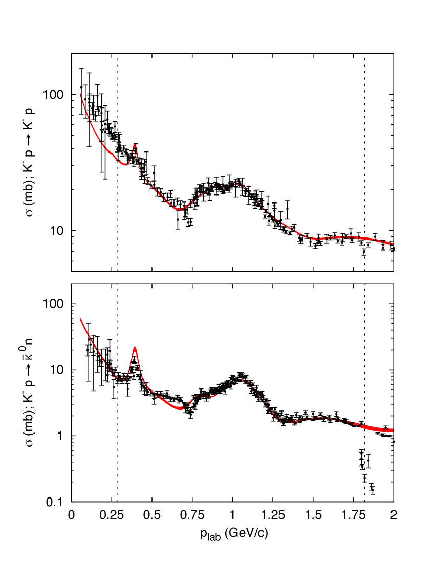
Figure 7: (color online). Cross sections for $K^{-}p\to K^{-}p,\bar{K}^{0}n$ processes. The vertical dashed lines mark the energy range where the single-energy partial waves have been fitted.

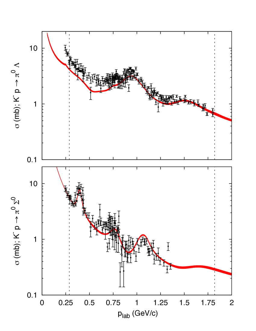
Figure 8: (color online). Cross sections for $K^{-}p\to\pi^{0}\Lambda,\pi^{0}\Sigma^{0}$ processes. The vertical dashed lines mark the energy range where the single-energy partial waves have been fitted.

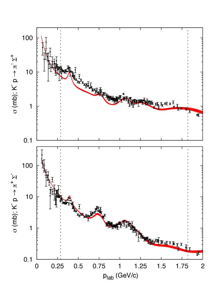
Figure 9: (color online). Cross sections for $K^{-}p\to\pi^{-}\Sigma^{+},\pi^{+}\Sigma^{-}$ processes. The vertical dashed lines mark the energy range where the single-energy partial waves have been fitted.

In this section we compare our model to the data on total cross sections (Section III.3.1, Figs. 7, 8, and 9), differential cross sections, and polarization observables (Section III.3.2, Figs. 10–19) for processes $\bar{K}N\to\bar{K}N$ Daum1968 ; Andersson1970 ; Albrow1971 ; Conforto1971 ; Adams1975 ; Abe1975 ; Mast1976 ; Alston1978 ; Armenteros1968 ; Armenteros1970 ; Jones1975 ; Griselin1975 ; Conforto1976 ; Prakhov2009 , $\bar{K}N\to\pi\Lambda$ Armenteros1968 ; Armenteros1970 ; Jones1975 ; Griselin1975 ; Conforto1976 ; Prakhov2009 ; Berthon1970a ; Baxter1973 ; London1975 ; Baldini1988 and $\bar{K}N\to\pi\Sigma$ Armenteros1968 ; Armenteros1970 ; Jones1975 ; Griselin1975 ; Conforto1976 ; Prakhov2009 ; Berthon1970b ; Baxter1973 ; London1975 ; Baldini1988 ; Manweiler2008 .

Because we have fitted the single-energy partial waves, their correlations are not incorporated in our analysis, which translates into missing an important piece of the error estimation in the observables. In order to account partly for that, we performed the following simulation. (i) For each partial wave we have picked randomly one of the 50 sets of parameters available from the bootstrap fits (cf. Section III.1). (ii) We have computed each partial wave. (iii) We have computed the observable. We have repeated this algorithm 1000 times to generate an average and standard deviation. Systematics are not considered in either the theoretical or the experimental error bars displayed and might be of importance in what regards to the cross sections, where a $\pm 10\%$ normalization effect is within experimental uncertainty.

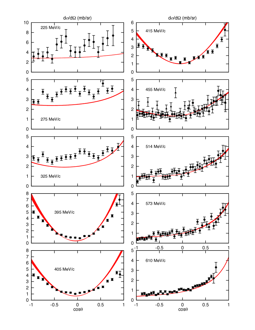
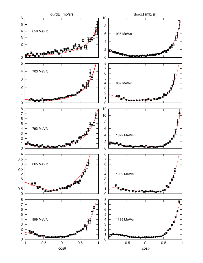
Figure 10: (color online). Differential cross-section ($d\sigma/d\Omega$), for the $K^{-}p\to K^{-}p$ process in terms of the cosine of the center-of-mass scattering angle $\theta$. The width of the theory bands correspond to the errors propagated from the partial waves to the observables as explained in the text. The momentum of the incoming $K^{-}$ in the laboratory frame is shown for each plot. Data from Andersson1970 ; Albrow1971 ; Conforto1971 ; Adams1975 ; Mast1976 ; Armenteros1970 ; Conforto1976 .

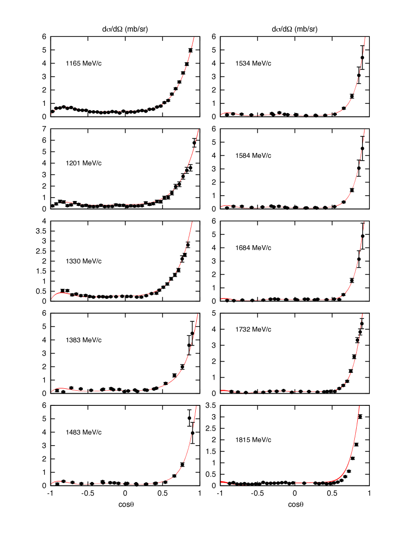
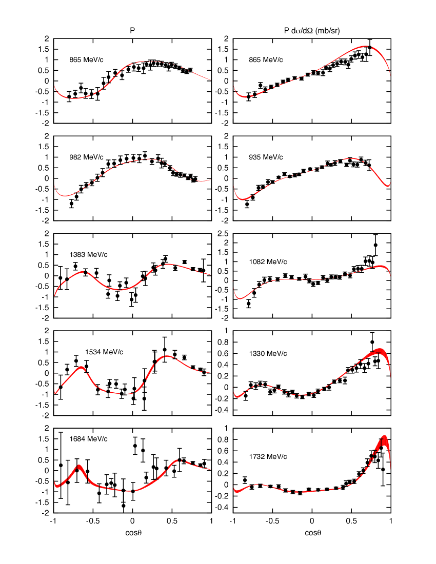
Figure 11: (color online). Differential cross-section ($\frac{d\sigma}{d\Omega}$, left and left-center columns) polarization asymmetry ($P$, right-center column), and $P\>\frac{d\sigma}{d\Omega}$ (right column) for the $K^{-}p\to K^{-}p$ process in terms of the cosine of the center-of-mass scattering angle $\theta$. The width of the theory bands correspond to the errors propagated from the partial waves to the observables as explained in the text. The momentum of the incoming $K^{-}$ in the laboratory frame is shown for each plot. Differential cross section data from Daum1968 ; Albrow1971 ; Abe1975 ; Andersson1970 ; Griselin1975 ; Conforto1976 , polarization data from Daum1968 ; Albrow1971 ; Andersson1970 , and $P\>\frac{d\sigma}{d\Omega}$ data from Albrow1971 ; Andersson1970 .

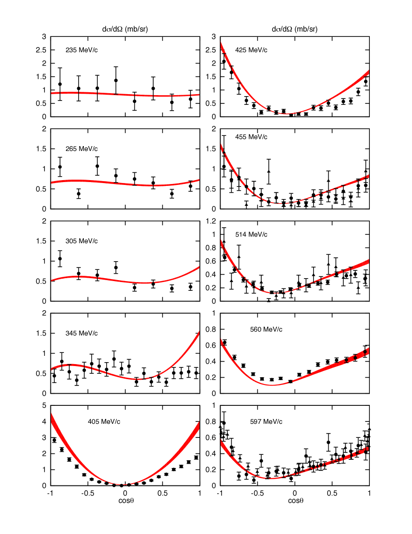
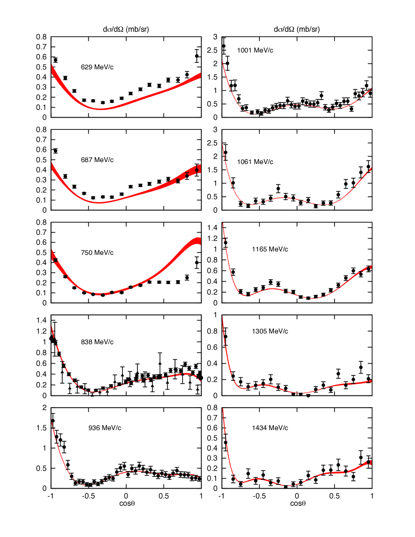
Figure 12: (color online). Same as Fig. 10 for the $K^{-}p\to\bar{K}^{0}n$ process. Data from Daum1968 ; Mast1976 ; Armenteros1970 ; Alston1978 ; Jones1975 ; Griselin1975 ; Conforto1976 ; Prakhov2009 .

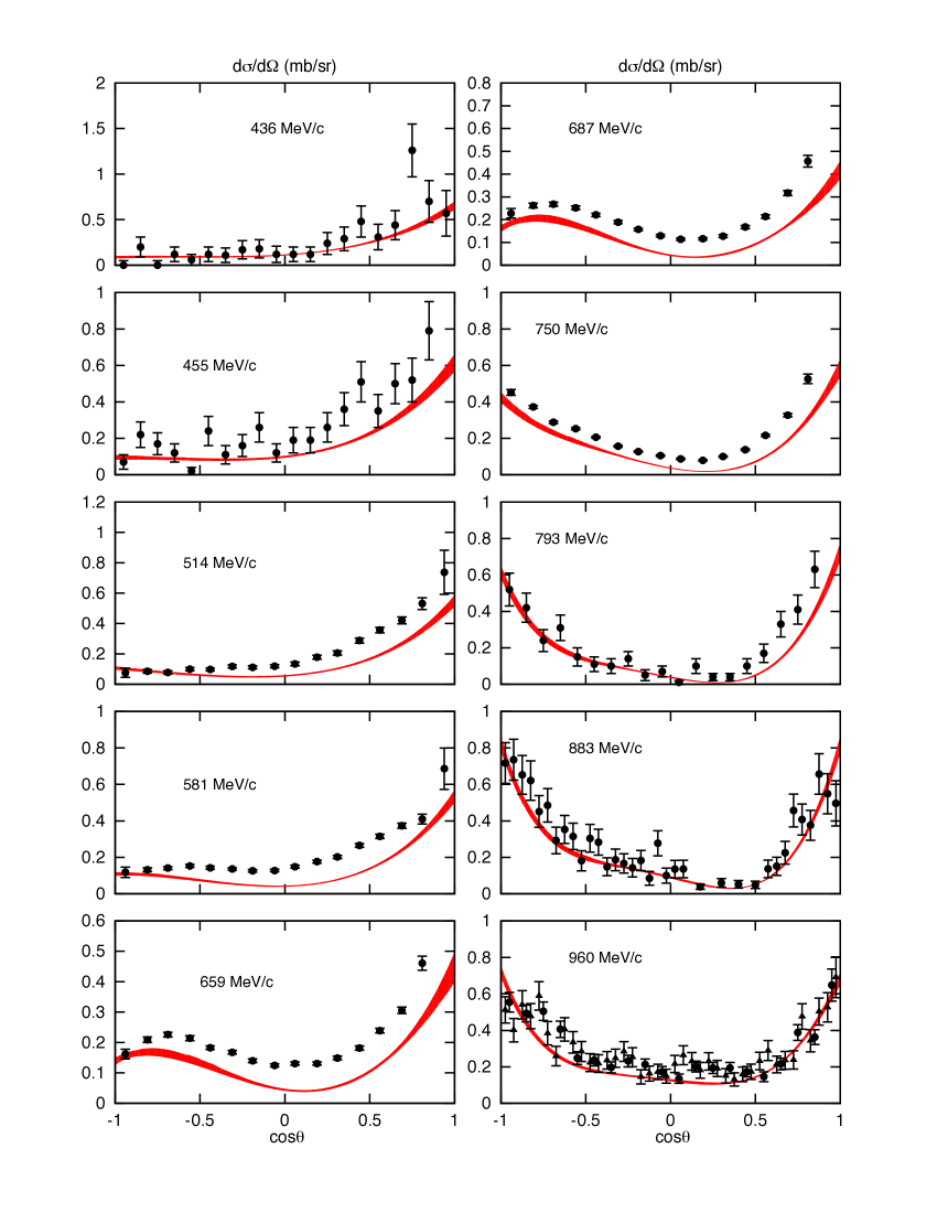
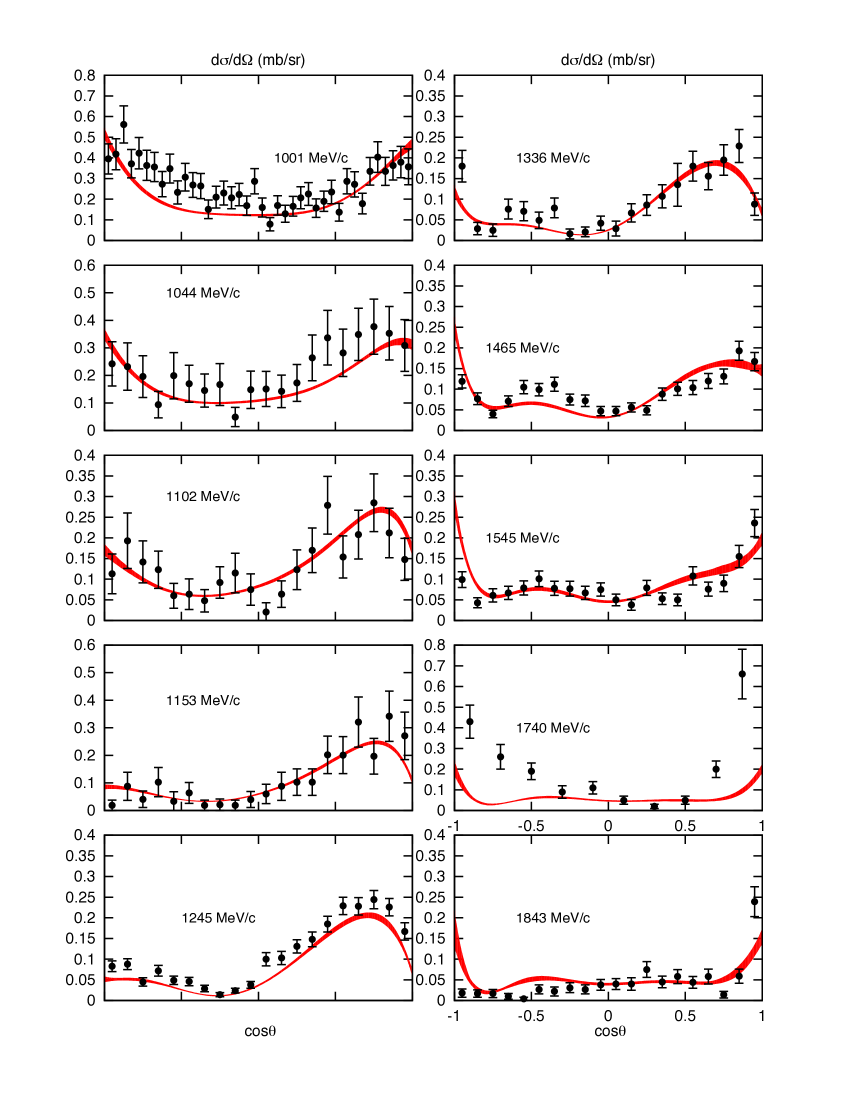
Figure 13: (color online). Same as Fig. 10 for the $K^{-}p\to\pi^{0}\Lambda$ process. Data from Armenteros1968 ; Armenteros1970 ; Jones1975 ; Griselin1975 ; Conforto1976 ; Berthon1970a ; London1975 ; Prakhov2009 .

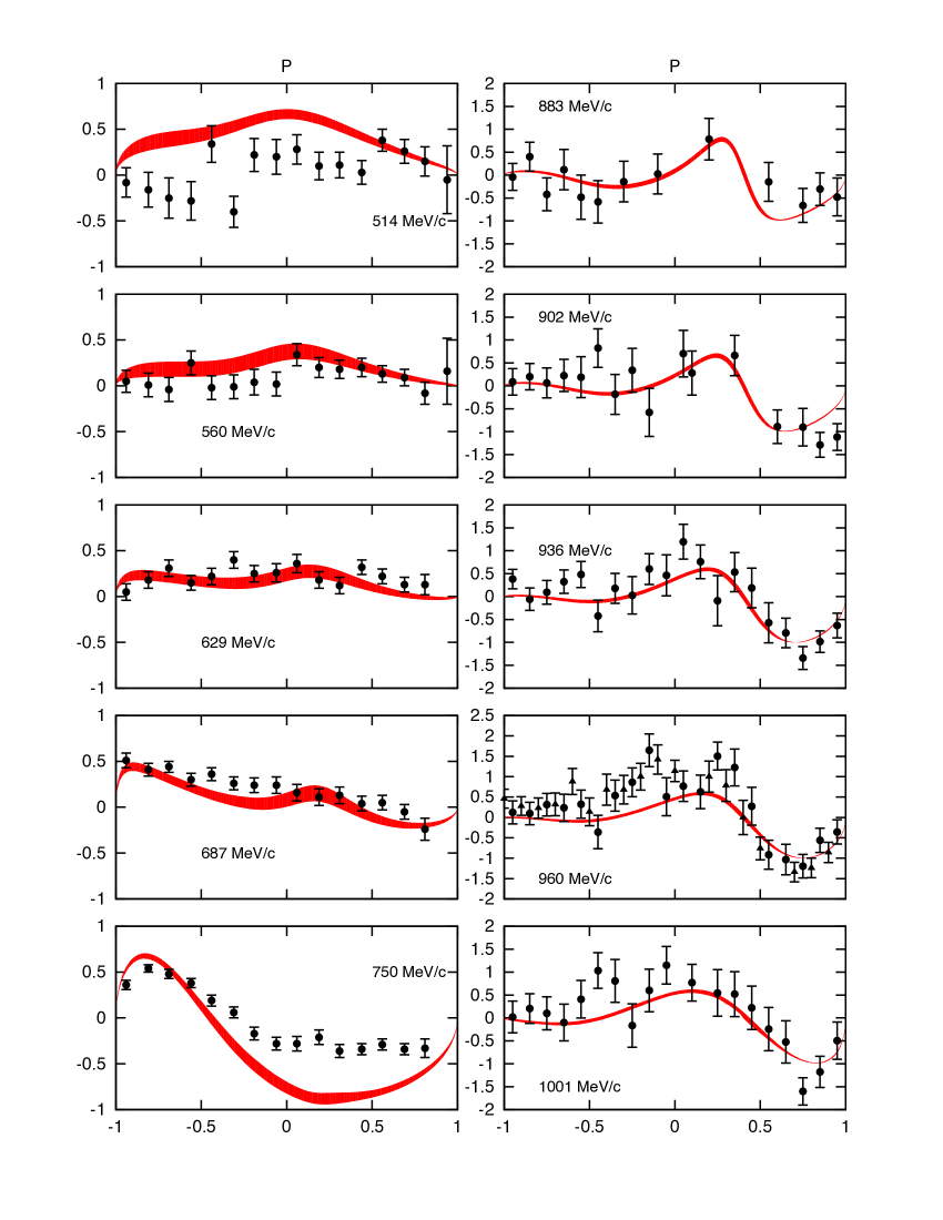
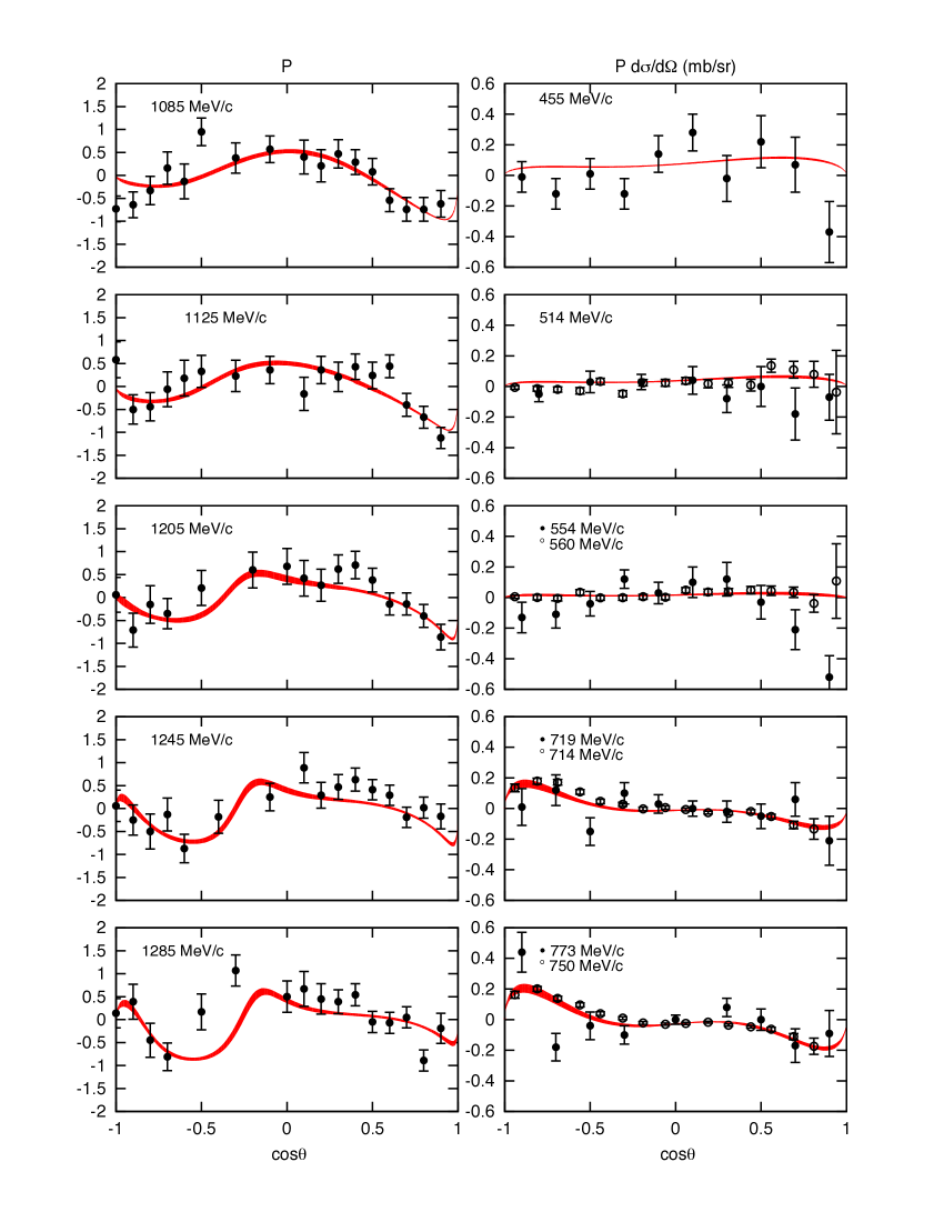
Figure 14: (color online). Polarization asymmetry ($P$, left, left-center and right-center columns), and $P\>\frac{d\sigma}{d\Omega}$ (right column) for the $K^{-}p\to\pi^{0}\Lambda$ process in terms of the cosine of the center-of-mass scattering angle $\theta$. Polarization data from Prakhov2009 for left column, from Conforto1976 for left-center column, and from Griselin1975 right-center column. $P\>\frac{d\sigma}{d\Omega}$ data from Armenteros1970 (solid circles) and Prakhov2009 (empty circles). For the last we have computed the error bars using standard error propagation from the $P$ and $d\sigma/d\Omega$ data. For plots where data are shown at two different energies the theory band has been computed at both energies.

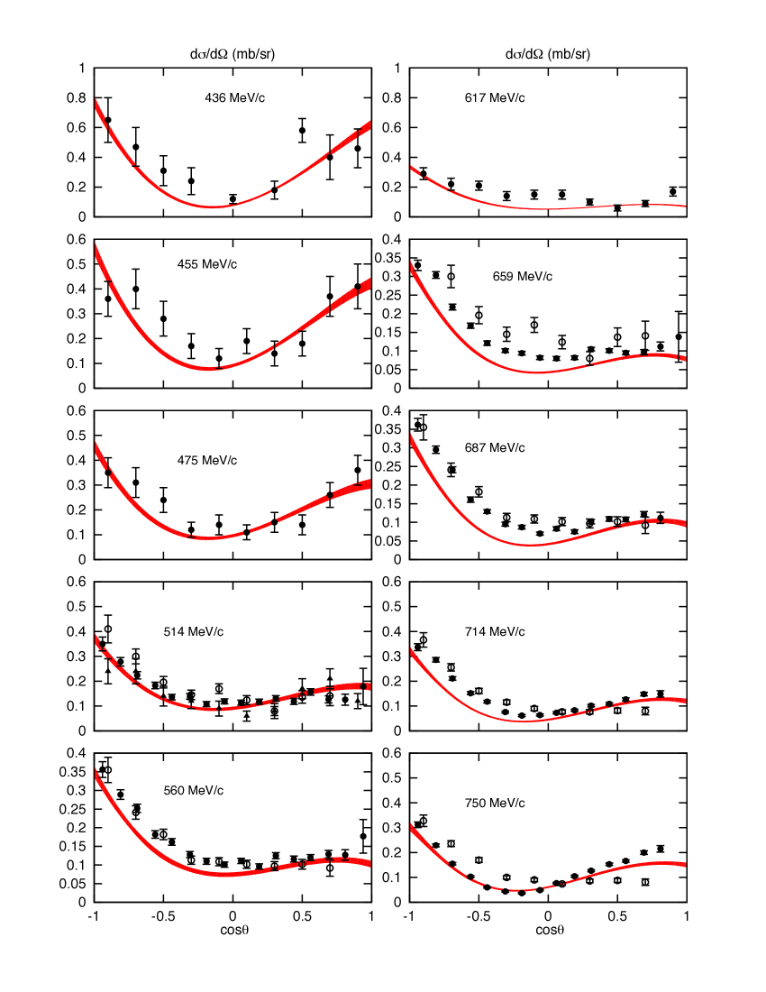
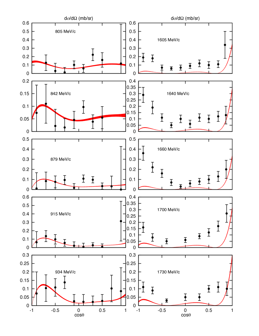
Figure 15: (color online). Same as Fig. 10 for the $K^{-}p\to\pi^{0}\Sigma^{0}$ process. Data at $p_{\text{lab}}=514,560,659,687,714$ and $750$ MeV$/c$ are from Prakhov2009 (solid circles), from Manweiler2008 (empty circles) and from Armenteros1970 (solid triangles only at 514 MeV$/c$). Remainder of the data from Armenteros1970 ; Baxter1973 ; London1975 .

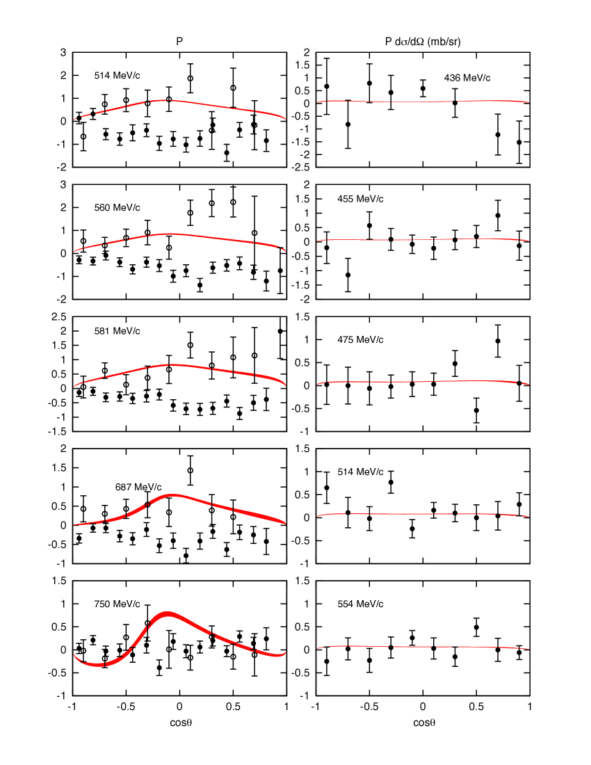
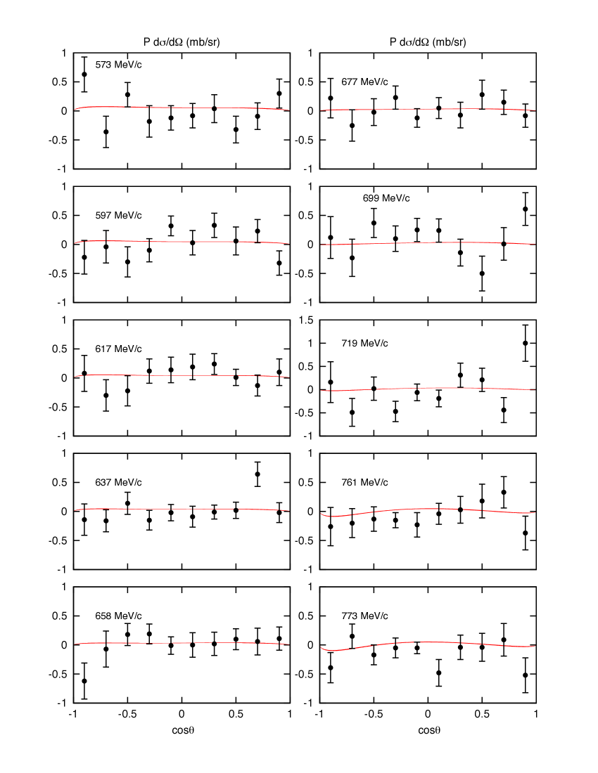
Figure 16: (color online). Polarization asymmetry ($P$, left column) and $P\>\frac{d\sigma}{d\Omega}$ (left-center, right-center and right columns) for the $K^{-}p\to\pi^{0}\Sigma^{0}$ process in terms of the cosine of the center-of-mass scattering angle $\theta$. Polarization data from Prakhov2009 , solid circles, and Manweiler2008 , empty circles. $P\>\frac{d\sigma}{d\Omega}$ data from Armenteros1970 .

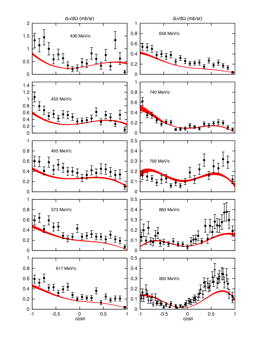
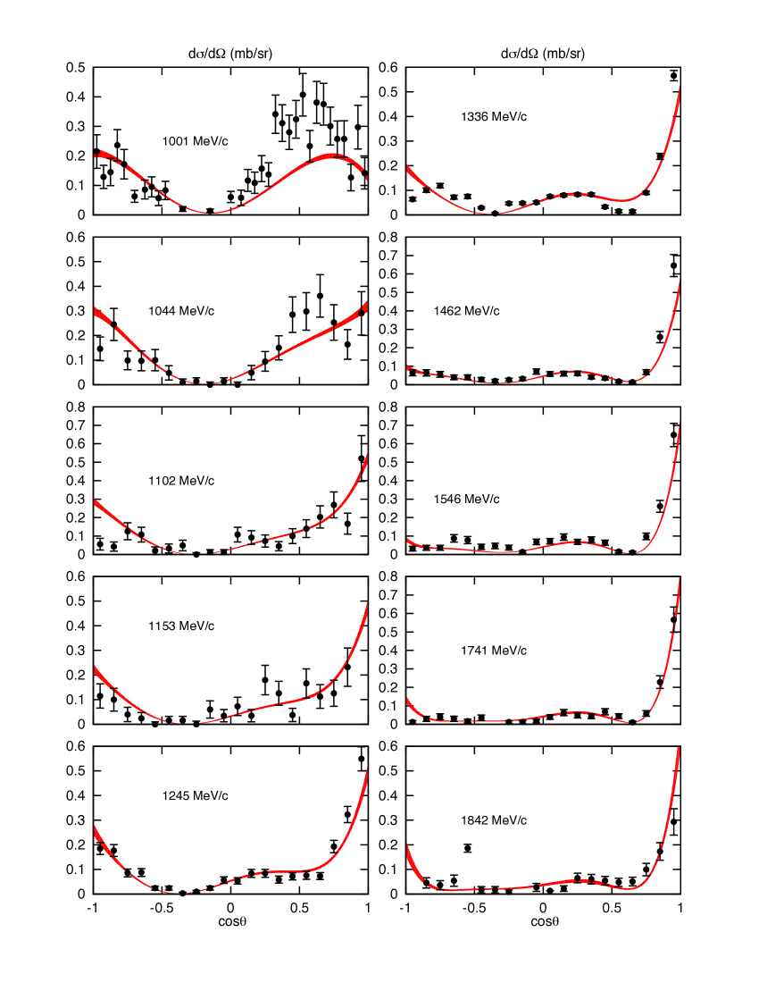
Figure 17: (color online). Same as Fig. 10 for the $K^{-}p\to\pi^{-}\Sigma^{+}$ process. Data from Armenteros1968 ; Armenteros1970 ; Jones1975 ; Griselin1975 ; Conforto1976 ; Berthon1970b .

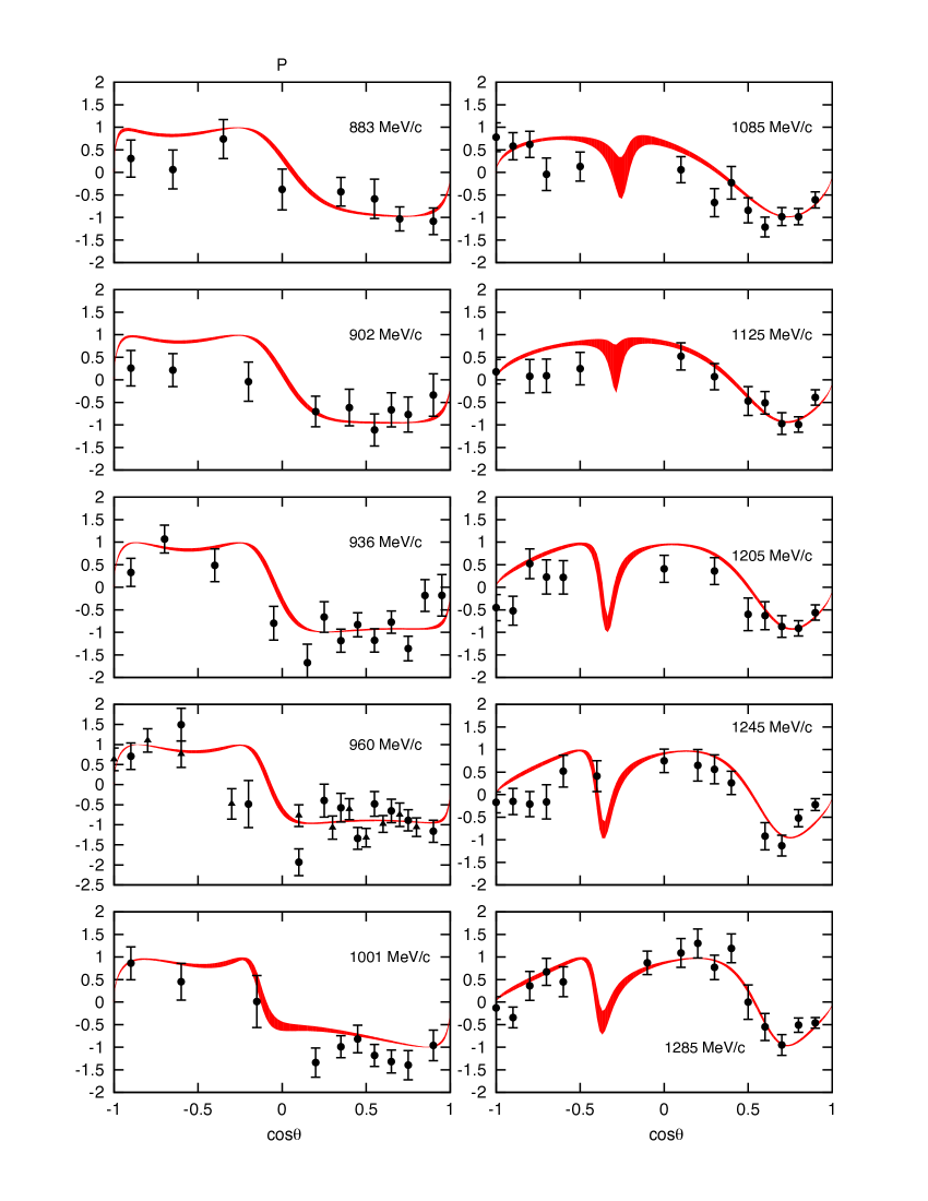
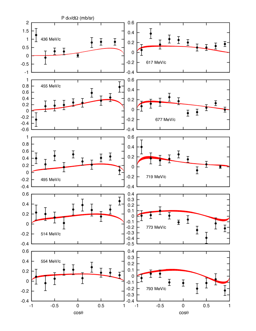
Figure 18: (color online). Polarization asymmetry ($P$, left and left-center columns) and $P\>\frac{d\sigma}{d\Omega}$ (right-center and right columns) for the $K^{-}p\to\pi^{-}\Sigma^{+}$ process in terms of the cosine of the center-of-mass scattering angle $\theta$. Polarization data from Jones1975 ; Conforto1976 and $P\>\frac{d\sigma}{d\Omega}$ data from Armenteros1970 .

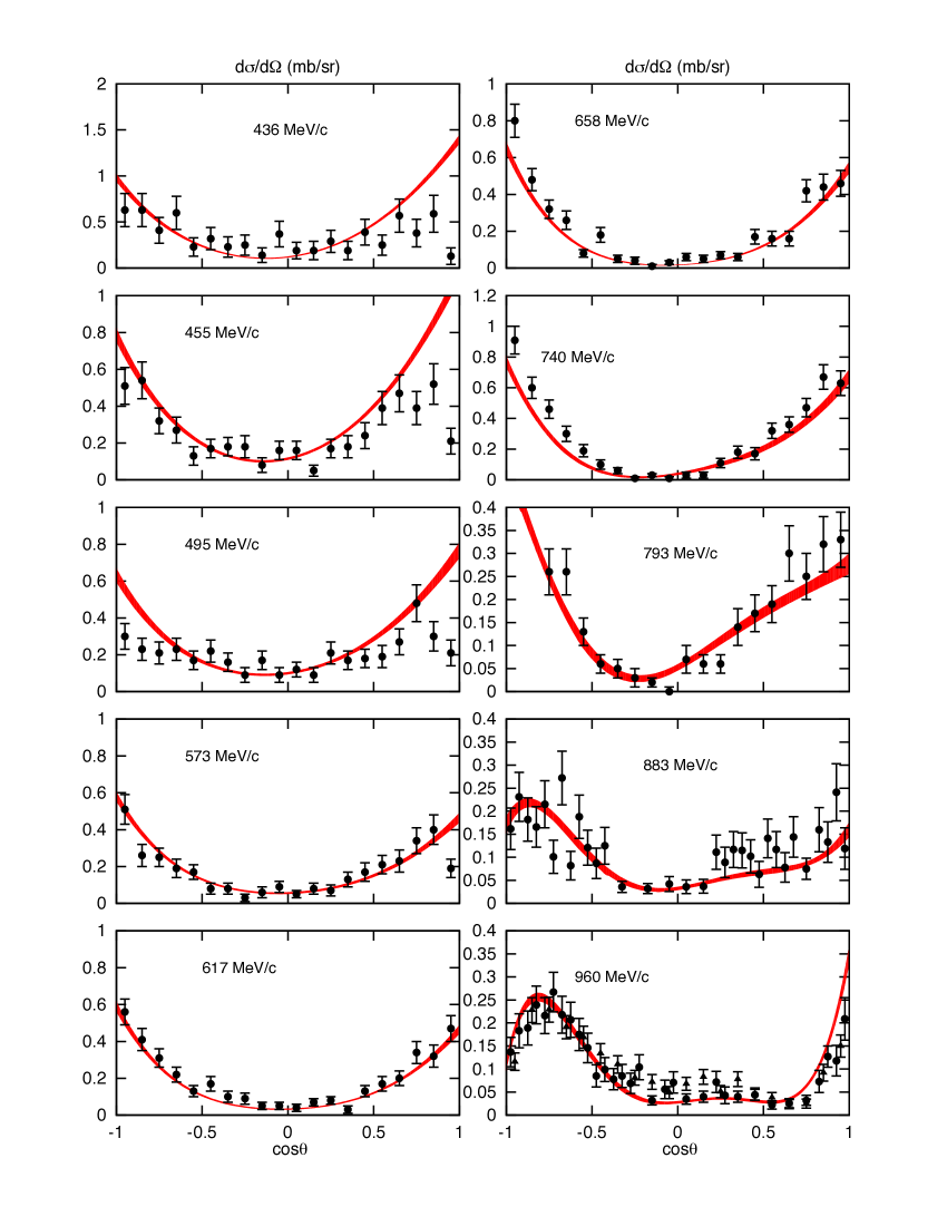
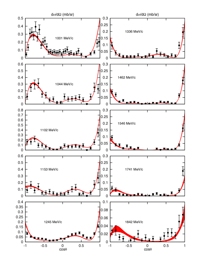
Figure 19: (color online). Same as Fig. 10 for the $K^{-}p\to\pi^{+}\Sigma^{-}$ process. Data from Armenteros1968 ; Armenteros1970 ; Jones1975 ; Griselin1975 ; Conforto1976 ; Berthon1970b .

III.3.1 Total Cross Sections

Figure 7 shows the total cross sections for $K^{-}p\to K^{-}p$ and $K^{-}p\to\bar{K}^{0}n$, which are the ones that matter the most for the future analysis of heavy meson decays and quasi-real diffractive photoproduction of $K\bar{K}$ on the proton at GluEx and CLAS12 JLAB . Both processes are well reproduced in the whole energy range. The $K^{-}p\to K^{-}p$ is underestimated below $p_{\text{lab}}=300$ MeV$/c$, although the general trend of the data is well described. We will revisit this discrepancy in Section III.3.2 where we compare to differential cross sections and polarizations.

Our results for $K^{-}p\to\pi^{0}\Lambda$ and $K^{-}p\to\pi^{0}\Sigma^{0}$ total cross sections are shown in Fig. 8. The uncertainties in the $K^{-}p\to\pi^{0}\Sigma^{0}$ process are very large and our model reproduces the total cross section very nicely except at $p_{\text{lab}}\simeq 600$ MeV$/c$, where we underestimate the observable. We obtain the general trend of the $K^{-}p\to\pi^{0}\Lambda$ data but they are poorly reproduced for $p_{\text{lab}}<800$ MeV$/c$ and $p_{\text{lab}}>1300$ MeV$/c$ as a direct consequence of our difficulties in describing the $S_{11}$ partial wave for $s<3$ GeV² and $s>3.9$ GeV² as shown in Fig 3. From the theoretical point of view, the $K^{-}p\to\pi^{0}\Lambda$ and $K^{-}p\to\pi^{0}\Sigma^{0}$ processes are very interesting. The first has only isospin-1 contributions ($\Sigma^{*}$’s) and the second has only isospin-0 contributions ($\Lambda^{*}$’s). This selectivity allows to decouple both sets of resonances and partial waves. However, in practice, both channels are difficult to separate experimentally Conforto1976 ; Prakhov2009 ; Manweiler2008 , which leads to systematic uncertainties in the data analysis. This is very well exposed if we compare total cross sections for two experimental data sets: Armenteros et al. Armenteros1970 and the most recent by Prakhov et al. Prakhov2009 in the energy region between $p_{\text{lab}}=450$ and $800$ MeV$/c$. For $K^{-}p\to\bar{K}^{0}n$ the agreement between both data sets is excellent as shown in Fig. 10 in Prakhov2009 . This indicates that uncertainties are well under control in both experiments for this reaction. However, for $K^{-}p\to\pi^{0}\Sigma^{0}$, Armenteros et al. shows a certain structure in the total cross section that, with better statistics and better control on the systematics, disappears in Prakhov et al., showing a flatter total cross section.

In Fig. 9 we display the $K^{-}p\to\pi^{\pm}\Sigma^{\mp}$ reactions. The $K^{-}p\to\pi^{+}\Sigma^{-}$ total cross section is very well reproduced except for the peak at $p_{\text{lab}}=750$ MeV$/c$ and the energy region between 1400 and 1750 MeV$/c$ where the observable is underestimated. The shape of the $K^{-}p\to\pi^{-}\Sigma^{+}$ total cross section is well reproduced although the absolute value of the observable is largely underestimated. The main source of disagreement is the inability of the model to provide a good description of the $S_{11}$ partial wave for the $\bar{K}N\to\pi\Sigma$ channel (Fig. 3) below $s=3$ GeV².

We find a certain level of inconsistency between the total cross section data for $K^{-}p\to\pi^{+}\Sigma^{-}$, $K^{-}p\to\pi^{0}\Sigma^{0}$ and $K^{-}p\to\pi^{-}\Sigma^{+}$ reactions. We reproduce $K^{-}p\to\pi^{0}\Sigma^{0}$ data, which have only isospin one contributions –see Eq. (9)– and we also reproduce $K^{-}p\to\pi^{+}\Sigma^{-}$ data whose amplitude is obtained as the isospin one amplitude minus the isospin zero amplitude. Hence, we should be able to predict correctly the $K^{-}p\to\pi^{-}\Sigma^{+}$ cross section, which corresponds to the addition of the two isospin amplitudes –see Eq. (7). Instead, we underestimate the $K^{-}p\to\pi^{-}\Sigma^{+}$ total cross section.

III.3.2 Differential Cross Sections and Polarizations

In this section we compare with the differential cross section and polarization data. Almost all of the database is from experiments performed during the late 60’s and the 70’s except for Prakhov2009 and Manweiler2008 published in 2009 and 2008, respectively. These two data sets come from the same BNL experiment and report measurements on the differential cross sections and polarizations for $K^{-}p\to\pi^{0}\Sigma^{0}$ Manweiler2008 ; Prakhov2009 and for $K^{-}p\to\bar{K}^{0}n$ and $K^{-}p\to\pi^{0}\Lambda$ Prakhov2009 for eight anti-kaon momenta. There are some discrepancies between these two data sets that will be apparent in the discussion of the $K^{-}p\to\pi^{0}\Sigma^{0}$ polarization.

We first compare to $K^{-}p\to K^{-}p$ and $K^{-}p\to\bar{K}^{0}n$ because one of our main interests is the $\bar{K}N\to\bar{K}N$ amplitude due to its importance in the rescattering of heavy-baryon decays and $K\bar{K}$ photoproduction experiments. The $\bar{K}N\to\bar{K}N$ data constitute almost half of the experimental database. However, the amount of polarization data is small with no data below $p_{\text{lab}}=865$ MeV$/c$ Albrow1971 . In Figs. 10 and 11 we compare our results to a wide sample of the $K^{-}p\to K^{-}p$ database. It is the best known reaction under consideration in this paper and the general description we obtain is excellent for both differential cross sections and polarizations. The only exceptions happen at low momenta, around $p_{\text{lab}}\simeq 400$ MeV$/c$, and at very high momentum, $p_{\text{lab}}=1815$ MeV$/c$. At low momentum we do not expect that a model like ours, built to describe the whole resonant region, provides an accurate description of the amplitude because we lack additional constrains like chiral symmetry that drives the physics at low energies. In the region around $p_{\text{lab}}\simeq 400$ MeV$/c$ ($\Lambda(1520)$ region) we capture the main behavior of the differential cross section although our model is not able to keep up with the rapid fall off of the cross section at forward and backward angles. This happens because, as shown in Section III.1, the variation of the single-energy partial-wave data is faster than the variation of the model, making difficult to capture the full extent of the partial wave in such region. At very high energy ($p_{\text{lab}}>1800$ MeV$/c$) our model overestimates the differential cross section, and is no longer very accurate, although it reproduces the trend of the data. We note the forward-angle behavior as the energy increases, which is the expected trend from Regge physics Mathieu15 .

We compare to $K^{-}p\to\bar{K}^{0}n$ differential cross sections in Fig. 12 (no polarization data are available). The overall agreement is very good. At $p_{\text{lab}}=345$ MeV$/c$ we find a large discrepancy at forward angles. The forward peak in the amplitude is due to the constructive interference between $P_{01}$, $P_{03}$, and $D_{03}$ partial waves, while at backward angles the interference between $P$ waves and $D_{03}$ is destructive. As for $K^{-}p\to K^{-}p$, the rapid variation of the amplitude due to the presence of the $\Lambda(1520)$ is not well reproduced and impacts the description of the data. The same explanation applies for the $p_{\text{lab}}=405$ MeV$/c$ data. Data points at $p_{\text{lab}}=560,629,687$ and $750$ MeV$/c$ and solid dots at $p_{\text{lab}}=514$ MeV$/c$ are from the most recent experiment in Ref. Prakhov2009 . These data have small statistical error bars and they were not used in the single-energy partial-wave amplitudes in Manley13b that we are fitting. We systematically underestimate the $p_{\text{lab}}=629$ MeV$/c$ and 687 MeV$/c$ data and we fail to reproduce the 750 MeV$/c$ data, where we find a larger forward contribution from the $P_{01}$, $P_{03}$ and specially $D_{03}$, $\Lambda(1690)$ contribution, that the other partial waves cannot compensate. In Prakhov2009 , the differential cross sections were fitted to Legendre polynomials expansion up to order five, rendering excellent fits for the $K^{-}p\to\bar{K}^{0}n$ data except for $p_{\text{lab}}=560,687$ and $750$ MeV$/c$. Hence, although we do not reproduce the 750 MeV$/c$ data, it is not worrisome because the data themselves might not be as good as they look according to their error bars. As the energy increases, experimental data are very well described.

The comparison to $K^{-}p\to\pi^{0}\Lambda$ differential cross sections is provided in Fig. 13 and to polarizations in Fig. 14. Only isospin-1 partial waves contribute to this reaction and as expected from the comparison to the total cross section, the energy region above $p_{\text{lab}}=790$ MeV$/c$ is very well described for differential cross sections except at $p_{\text{lab}}=1740$ MeV$/c$ ($s=4.52$ GeV${}^{2}/c^{2}$). This energy corresponds to the upper limit of the fitted energy region and neither the magnitude nor the shape of the cross section are properly reproduced. The shape of the the low-energy cross sections is correctly obtained but we fail to recover the right magnitude mainly due to our poor description of the $S_{11}$ partial wave.

We have a good description of the polarization data in Fig. 14 with the exception of $p_{\text{lab}}=514,960$ and $750$ MeV$/c$. Despite the fact that we do not obtain the correct magnitude of the differential cross section or polarization at 514 MeV$/c$ and 750 MeV$/c$ we do obtain both magnitude and shape for the $P\frac{d\sigma}{d\Omega}$ observable. This is specially puzzling in the case of 750 MeV$/c$ where the discrepancy between theory and experiment is very apparent.

Polarization data are experimentally very challenging for the $K^{-}p\to\pi^{0}\Lambda$ and $K^{-}p\to\pi^{0}\Sigma^{0}$. These difficulties become obvious when we compare to $K^{-}p\to\pi^{0}\Sigma^{0}$ polarization data from Refs. Prakhov2009 ; Manweiler2008 . For $P\frac{d\sigma}{d\Omega}$ we compare to data from Armenteros1970 for $p_{\text{lab}}=455,514,554,719$ and $773$ MeV$/c$ and we construct the observable from the differential cross section and the polarization observable from the most recent data in Prakhov2009 for the closest possible momenta $p_{\text{lab}}=514,560,714$ and $750$ MeV$/c$. In this way it is possible to observe the improvement these latest data constitute. For example, at $p_{\text{lab}}=554$ (560) MeV$/c$ the forward and backward structures disappear obtaining a flatter distribution and at 719 (714) and 773 (750) MeV$/c$ any disagreement between theory and experiment vanishes. Hence, disagreements at 960 and 1285 MeV$/c$ for $P$ and at 455 MeV$/c$ for $P\frac{d\sigma}{d\Omega}$ are not worrisome.

The measurement of the $K^{-}p\to\pi^{0}\Sigma^{0}$ reaction is very challenging. An excellent example of the difficulties is provided by the only two experimental papers in the last 35 years on $K^{-}p$ scattering, which have tried to tackle this reaction, i.e. Manweiler et al. Manweiler2008 and Prakhov et al. Prakhov2009 . Both analyses have been performed on the same experimental data at eight incident $K^{-}$ momenta ($p_{\text{lab}}=514,560,581,629,659,687,714$, and $750$ MeV$/c$) reporting overall normalization uncertainties of $\pm 7\%$ Prakhov2009 and $\pm 10\%$ Manweiler2008 with serious disagreements on the systematic uncertainties treatment and their results, specially at forward angles. Figure 15 shows a sample of $K^{-}p\to\pi^{0}\Sigma^{0}$ differential cross sections and in particular data from these two analyses at six momenta. Both analyses agree for the lower energies but the discrepancies are very apparent at the higher energies. This situation gets worse if we compare the polarization results as we do in the first column in Fig. 16, where they disagree even in the sign of the polarization at every momenta except at 750 MeV$/c$, which has very large error bars. The KSU single-energy partial waves that we have fitted incorporated the data from Manweiler2008 but not the data from Prakhov2009 in their extraction. This explains why our model has better agreement with the polarization data from Manweiler2008 . In Fig. 16 we also compare to the $P\frac{d\sigma}{d\Omega}$ from Armenteros1970 although the large error bars make difficult any meaningful comparison between theory and experiment. At high energies, the differential cross section is not well reproduced as it is obvious from the fourth column in Fig. 15. The KSU single-energy partial waves we have fitted do not reproduce these high-energy $K^{-}p\to\pi^{0}\Sigma^{0}$ data, hence we do not expect to reproduce them with our model.

As expected from the results on the total cross section, the differential cross sections are systematically underestimated at low energies for the $K^{-}p\to\pi^{-}\Sigma^{+}$ reaction as it is shown in Fig. 17. We underestimate the peak at $\cos\theta\simeq 0.7$ that shows up for $p_{\text{lab}}$ from $\sim 790$ MeV$/c$ to $\sim 1100$ MeV$/c$. The peak shape is generated by the $F_{05}$ partial wave and its magnitude by its interference with $P_{03}$ wave. If we compare both partial waves for the $\bar{K}N\to\pi\Sigma$ channel in the energy range between 2 and 3 GeV² in Figs. 1 ($2^{\text{nd}}$ row, $3^{\text{rd}}$ column) and 2 ($2^{\text{nd}}$ row, $2^{\text{nd}}$ column) we find that there is a sizable underestimation of the single-energy partial waves by our fits that are responsible for the result we obtain for the differential cross sections. This explains also the deviation from the $P\frac{d\sigma}{d\Omega}$ data in Fig. 18 at the same energies (although polarization data are fairly well reproduced). The rest of the polarization and $P\frac{d\sigma}{d\Omega}$ data are well reproduced considering the large uncertainties and that many experimental data points have unphysical values of $|P|>1$. Unfortunately, in the angular region for the polarization data ($\cos\theta\simeq-0.25$) where the most interesting structure shows up we lack experimental information.

The comparison to $K^{-}p\to\pi^{+}\Sigma^{-}$ differential cross sections is presented in Fig. 19. No polarization data are available for this reaction. The agreement between theory and experiment is excellent for all energies and angles except for the forward region at low energies (see $p_{\text{lab}}=436,455$, and $495$ MeV$/c$) where the reduction of the differential cross section can be achieved through the interference of $D_{05}$ with higher-order partial waves, however, $D_{03}$ contribution compensates $D_{05}$ and $P_{01}$, $P_{13}$ and $D_{13}$ contribute to the large overestimation shown in the plots. Nevertheless, all the low-energy experimental points come from the same experiment in Ref. Armenteros1970 and further independent experimental information would be useful.

IV Conclusions and Outlook

We have presented a coupled-channel model for $\bar{K}N,\pi\Sigma,\ldots\to\bar{K}N,\pi\Sigma,\ldots$ processes in the resonant region (up to $s=4.70$ GeV²) incorporating all the relevant channels. The approach presented is based on $K$-matrix formalism and Breit–Wigner parameterizations. The $T$ matrix is analytical, the first Riemann sheet has no poles (at least in a very wide area that envelopes the physical region of interest). Unitarity gives the discontinuity of the $T$-matrix elements across the right-hand cuts and determines continuation to complex values of $s$ below the real axis where resonance poles are located in the unphysical Riemann sheets. Analytical amplitudes enable the application of dispersion relations to connect the resonance region with the high-energy domain that is dominated by Regge poles in cross-channels, e.g. in a similar fashion to that used recently in the analysis of $\pi N$ scattering Mathieu15 . The construction of amplitudes valid in a wide range of energies is required in the analysis of processes that have $\bar{K}N$ in the final states, e.g. three-body decays to $\bar{K}N+$meson in pentaquark searches LHCbpentaquark and real and quasi-real diffractive photoproduction of $K\bar{K}$ pairs on the proton in the search for strangeonia and exotic mesons with hidden strangeness JLAB .

For simplicity and computational reasons we have fitted our model to the single-energy partial waves from Manley13a . We present the results of our fits in Table 1 and Figs. 1–4. Statistical errors have been estimated by means of the bootstrap technique. In general the fits obtained are very good except for $S_{01}$, $P_{01}$ and $S_{11}$ partial waves, whose resonance extraction is less reliable than for other partial waves. For these three partial waves we have performed additional analyses on systematic errors by randomly pruning and refitting the data base. Due to their nature, these systematic uncertainties have not been propagated to the resonances or observables error estimation.

We have reported the most comprehensive analysis of the $Y^{*}$ spectrum to date. All the obtained resonances are summarized in Tables 2 and 3 together with their uncertainties and a comparison to previous pole extractions by Zhang et al. Manley13b and Kamano et al. Kamano15 . We provide graphical representations of the location of the resonances in Fig. 5 ($T$-matrix pole positions in the unphysical Riemann sheets) and Fig. 6 (Regge trajectories). The Regge trajectories provide additional insight into the nature of the hyperon spectrum. Gaps in the trajectories provide hints on possible missing states and the shape of the trajectories and their (non-)linearity information on the quark-gluon dynamics reggetrajectories . We find that most of the states fit within linear trajectories, implying a three-quark state nature. An exception is the $\Lambda(1600)$ whose mass and width are very well established and does not fit within the daughter natural parity linear Regge trajectory. Hence, it is likely that its nature is not that of a three-quark state. We report a $3/2^{+}$ state in the $P_{03}$ partial wave with a mass of $1690$ MeV and a narrow width of 46 MeV that fills in the gap in the parent $0^{-}$ Regge trajectory (see Fig. 6(a)). A similar $P_{03}$ state was found in Kamano15 at $M_{p}=1671$ MeV and $\Gamma_{p}=10$ MeV, although with a model that does not obtain the four-star $\Lambda(1830)$ state also present in the $P_{03}$ partial wave. Neither present nor Manley13b ; Kamano15 analyses find evidence of the three-star $\Sigma(1940)$ state in the $D_{13}$ partial wave, however, the structure of the Regge trajectories in Fig. 6(b) suggests that this state is necessary to fill in a gap in the $1^{+}$ daughter Regge trajectory and further studies are mandatory.

Finally, we have compared our model predictions to the experimental observables for $K^{-}p\to K^{-}p$, $\bar{K}^{0}n$, $\pi^{0}\Lambda$, $\pi^{0}\Sigma^{0}$, $\pi^{-}\Sigma^{+}$, $\pi^{+}\Sigma^{-}$ reactions, namely, total and differential cross sections, polarizations and $P\frac{d\sigma}{d\Omega}$. The $K^{-}p\to K^{-}p$ and $K^{-}p\to\bar{K}^{0}n$ data are well reproduced and our amplitudes are an adequate input for $\bar{K}N+$meson decays and $\gamma p\to K\bar{K}p$ partial-wave analyses. The model also provides a general good description for $K^{-}p\to\pi^{+}\Sigma^{-}$ and $K^{-}p\to\pi^{0}\Sigma^{0}$ processes and a not-so-good description of the $K^{-}p\to\pi^{-}\Sigma^{+}$ and $K^{-}p\to\pi^{0}\Lambda$ reactions depending on the energy range under consideration. The reasons for discrepancies, database inconsistencies and systematics have been addressed in Section III.3.

The next step in a comprehensive description and analysis of the hyperon spectrum consists on fitting directly the experimental data as done in Kamano14 bypassing the single-energy partial waves from Manley13a . The partial waves presented in this paper can be used as starting point in the fitting process. The examination of the experimental database shows how in dire need of new data we are due to discrepancies encountered between different experimental analyses. Considering how increasingly important $\bar{K}N$ amplitudes are becoming in the data analysis for hadron spectroscopy research programs at LHCb LHCbpentaquark and Jefferson Lab JLAB an ambitious experimental program should be seriously considered in the future experimental research programs at hadron beam facilities KNstatus .

The codes employed to compute the partial waves and the observables are available for downloading as well as in an interactive form online at the Joint Physics Analysis Center (JPAC) webpage JPACwebpage .

Appendix A Solution to Eqs. (42) and (43)

In this Appendix we provide the analytic expressions of $c_{ab}(s)$ and $\mathcal{D}(s)$ for the case of six $K$ matrices that satisfy the system of equations defined by Eqs. (42) and (43). Throughout this Appendix we drop the $s$ dependence in the equations. The solution reads:

$$c_{aa}=\mathcal{T}_{a}\left(1+2i\>f_{bcdef}\mathcal{T}_{bcdef}+\sum_{\{j,k\}}\varepsilon_{jk}\mathcal{T}_{jk}+2i\>\sum_{\{j,k,l\}}f_{jkl}\>\mathcal{T}_{jkl}+\sum_{\{j,k,l,m\}}f_{jklm}\mathcal{T}_{jklm}\right)\>,$$ (45)

$$c_{ab}=i\varepsilon_{ab}\mathcal{T}_{a}\mathcal{T}_{b}\left(1+\sum_{\{j,k\}}\varepsilon_{jk}\mathcal{T}_{jk}+2i\>\sum_{\{j,k,l\}}f_{jkl}\>\mathcal{T}_{jkl}+\sum_{\{j,k,l,m\}}f_{jklm}\mathcal{T}_{jklm}+2i\>f_{jklmn}\mathcal{T}_{jklmn}\right)\>,\quad a\neq b\>;$$ (46)

$$\mathcal{D}=1+\sum_{\{j,k\}}\varepsilon_{jk}^{2}\>\mathcal{T}_{jk}+2i\>\sum_{\{j,k,l\}}f_{jkl}\>\mathcal{T}_{jkl}+\sum_{\{j,k,l,m\}}f_{jklm}\mathcal{T}_{jklm}+2i\>\sum_{\{j,k,l,m,n\}}f_{jklmn}\mathcal{T}_{jklmn}+f_{123456}\mathcal{T}_{123456}\>,$$ (47)

where we define $\{j,k\}$, $\{j,k,l\}$, $\{j,k,l,m\}$ and $\{j,k,l,m,n\}$ as the set of combinations without repetition of six elements taken in sets of two, three, four, and five elements at a time, respectively, where $1$ to $6$ label each one of the $K_{a}$ matrices. In Eqs. (45) and (46) $a,b\neq j,k,l,m,n$. $\varepsilon_{ij}$ is defined by Eq. (44). The $\mathcal{T}$’s are defined by

$$\mathcal{T}_{123456} = \mathcal{T}_{1}\>\mathcal{T}_{2}\>\mathcal{T}_{3}\>\mathcal{T}_{4}\>\mathcal{T}_{5}\>\mathcal{T}_{6}\>,$$ (48)

$$\mathcal{T}_{jklmn} = \mathcal{T}_{j}\>\mathcal{T}_{k}\>\mathcal{T}_{l}\>\mathcal{T}_{m}\>\mathcal{T}_{n}\>,$$ (49)

$$\mathcal{T}_{jklm} = \mathcal{T}_{j}\>\mathcal{T}_{k}\>\mathcal{T}_{l}\>\mathcal{T}_{m}\>,$$ (50)

$$\mathcal{T}_{jkl} = \mathcal{T}_{j}\>\mathcal{T}_{k}\>\mathcal{T}_{l}\>,$$ (51)

$$\mathcal{T}_{jk} = \mathcal{T}_{j}\>\mathcal{T}_{k}\>,$$ (52)

where $\mathcal{T}_{j}$ is defined by Eq. (26) if $j$ denotes a pole $K$ matrix and by Eq. (29) if $j$ denotes a background $K$ matrix.

The $f$ functions are defined as follows:

$$f_{jkl}=\varepsilon_{jk}\varepsilon_{kl}\varepsilon_{lj}\>,$$ (54)

$$\begin{split}f_{ijkl}=&\>\varepsilon_{il}^{2}\>\varepsilon_{jk}^{2}+\varepsilon_{ij}^{2}\>\varepsilon_{kl}^{2}+\varepsilon_{ik}^{2}\>\varepsilon_{jl}^{2}-2\>\varepsilon_{ij}\>\varepsilon_{ik}\>\varepsilon_{jl}\>\varepsilon_{kl}\\ &-2\>\varepsilon_{ik}\>\varepsilon_{il}\>\varepsilon_{jk}\>\varepsilon_{jl}-2\>\varepsilon_{ij}\>\varepsilon_{il}\>\varepsilon_{jk}\>\varepsilon_{kl}\>,\end{split}$$ (55)

$$\begin{split}f_{ijklm}=&\>\varepsilon_{im}^{2}\varepsilon_{jk}\varepsilon_{jl}\varepsilon_{kl}+\varepsilon_{ik}\varepsilon_{il}\varepsilon_{jm}^{2}\varepsilon_{kl}\\ +&\>\varepsilon_{ij}\varepsilon_{im}\varepsilon_{jm}\varepsilon_{kl}^{2}+\varepsilon_{ik}\varepsilon_{im}\varepsilon_{jl}^{2}\varepsilon_{km}\\ +&\>\varepsilon_{il}^{2}\varepsilon_{jk}\varepsilon_{jm}\varepsilon_{km}+\varepsilon_{ij}\varepsilon_{il}\varepsilon_{jl}\varepsilon_{km}^{2}\\ +&\>\varepsilon_{il}\varepsilon_{im}\varepsilon_{jk}^{2}\varepsilon_{lm}+\varepsilon_{ik}^{2}\varepsilon_{jl}\varepsilon_{jm}\varepsilon_{lm}\\ +&\>\varepsilon_{ij}^{2}\varepsilon_{kl}\varepsilon_{km}\varepsilon_{lm}+\varepsilon_{ij}\varepsilon_{ik}\varepsilon_{jk}\varepsilon_{lm}^{2}\\ -&\>\varepsilon_{il}\varepsilon_{im}\varepsilon_{jk}\varepsilon_{jm}\varepsilon_{kl}-\varepsilon_{ik}\varepsilon_{im}\varepsilon_{jl}\varepsilon_{jm}\varepsilon_{kl}\\ -&\>\varepsilon_{il}\varepsilon_{im}\varepsilon_{jk}\varepsilon_{jl}\varepsilon_{km}-\varepsilon_{ik}\varepsilon_{il}\varepsilon_{jl}\varepsilon_{jm}\varepsilon_{km}\\ -&\>\varepsilon_{ij}\varepsilon_{im}\varepsilon_{jl}\varepsilon_{kl}\varepsilon_{km}-\varepsilon_{ij}\varepsilon_{il}\varepsilon_{jm}\varepsilon_{kl}\varepsilon_{km}\\ -&\>\varepsilon_{ik}\varepsilon_{im}\varepsilon_{jk}\varepsilon_{jl}\varepsilon_{lm}-\varepsilon_{ik}\varepsilon_{il}\varepsilon_{jk}\varepsilon_{jm}\varepsilon_{lm}\\ -&\>\varepsilon_{ij}\varepsilon_{im}\varepsilon_{jk}\varepsilon_{kl}\varepsilon_{lm}-\varepsilon_{ij}\varepsilon_{ik}\varepsilon_{jm}\varepsilon_{kl}\varepsilon_{lm}\\ -&\>\varepsilon_{ij}\varepsilon_{il}\varepsilon_{jk}\varepsilon_{km}\varepsilon_{lm}-\varepsilon_{ij}\varepsilon_{ik}\varepsilon_{jl}\varepsilon_{km}\varepsilon_{lm}\>,\end{split}$$ (56)

$$f_{123456}=\>\alpha-4\beta+2\left(\gamma_{1}+\gamma_{2}-\delta_{1}-\delta_{2}\right)\>,$$ (57)

where

$$\begin{split}\alpha=&\>\varepsilon_{16}^{2}\varepsilon_{25}^{2}\varepsilon_{34}^{2}+\varepsilon_{15}^{2}\varepsilon_{26}^{2}\varepsilon_{34}^{2}+\varepsilon_{16}^{2}\varepsilon_{24}^{2}\varepsilon_{35}^{2}+\varepsilon_{14}^{2}\varepsilon_{26}^{2}\varepsilon_{35}^{2}+\varepsilon_{15}^{2}\varepsilon_{24}^{2}\varepsilon_{36}^{2}+\varepsilon_{14}^{2}\varepsilon_{25}^{2}\varepsilon_{36}^{2}\\ +&\>\varepsilon_{12}^{2}\varepsilon_{35}^{2}\varepsilon_{46}^{2}+\varepsilon_{13}^{2}\varepsilon_{24}^{2}\varepsilon_{56}^{2}+\varepsilon_{16}^{2}\varepsilon_{23}^{2}\varepsilon_{45}^{2}+\varepsilon_{12}^{2}\varepsilon_{36}^{2}\varepsilon_{45}^{2}+\varepsilon_{13}^{2}\varepsilon_{26}^{2}\varepsilon_{45}^{2}+\varepsilon_{12}^{2}\varepsilon_{34}^{2}\varepsilon_{56}^{2}\\ +&\>\varepsilon_{14}^{2}\varepsilon_{23}^{2}\varepsilon_{56}^{2}+\varepsilon_{13}^{2}\varepsilon_{25}^{2}\varepsilon_{46}^{2}+\varepsilon_{15}^{2}\varepsilon_{23}^{2}\varepsilon_{46}^{2}\>,\end{split}$$ (58)

$$\begin{split}\beta=&\>\varepsilon_{12}\varepsilon_{13}\varepsilon_{23}\varepsilon_{45}\varepsilon_{46}\varepsilon_{56}+\varepsilon_{12}\varepsilon_{14}\varepsilon_{24}\varepsilon_{35}\varepsilon_{36}\varepsilon_{56}+\varepsilon_{12}\varepsilon_{16}\varepsilon_{26}\varepsilon_{34}\varepsilon_{35}\varepsilon_{45}+\varepsilon_{13}\varepsilon_{16}\varepsilon_{24}\varepsilon_{25}\varepsilon_{36}\varepsilon_{45}\\ +&\>\varepsilon_{14}\varepsilon_{15}\varepsilon_{23}\varepsilon_{26}\varepsilon_{36}\varepsilon_{45}+\varepsilon_{14}\varepsilon_{16}\varepsilon_{23}\varepsilon_{25}\varepsilon_{35}\varepsilon_{46}+\varepsilon_{13}\varepsilon_{15}\varepsilon_{24}\varepsilon_{26}\varepsilon_{35}\varepsilon_{46}+\varepsilon_{12}\varepsilon_{15}\varepsilon_{25}\varepsilon_{34}\varepsilon_{36}\varepsilon_{46}\\ +&\>\varepsilon_{15}\varepsilon_{16}\varepsilon_{23}\varepsilon_{24}\varepsilon_{34}\varepsilon_{56}+\varepsilon_{13}\varepsilon_{14}\varepsilon_{25}\varepsilon_{26}\varepsilon_{34}\varepsilon_{56}\>,\end{split}$$ (59)

$$\begin{split}\gamma_{1}=&\>\varepsilon_{15}\varepsilon_{16}\varepsilon_{24}\varepsilon_{26}\varepsilon_{34}\varepsilon_{35}+\varepsilon_{14}\varepsilon_{16}\varepsilon_{25}\varepsilon_{26}\varepsilon_{34}\varepsilon_{35}+\varepsilon_{15}\varepsilon_{16}\varepsilon_{24}\varepsilon_{25}\varepsilon_{34}\varepsilon_{36}+\varepsilon_{14}\varepsilon_{15}\varepsilon_{25}\varepsilon_{26}\varepsilon_{34}\varepsilon_{36}\\ +&\>\varepsilon_{14}\varepsilon_{16}\varepsilon_{24}\varepsilon_{25}\varepsilon_{35}\varepsilon_{36}+\varepsilon_{14}\varepsilon_{15}\varepsilon_{24}\varepsilon_{26}\varepsilon_{35}\varepsilon_{36}+\varepsilon_{15}\varepsilon_{16}\varepsilon_{23}\varepsilon_{26}\varepsilon_{34}\varepsilon_{45}+\varepsilon_{13}\varepsilon_{16}\varepsilon_{25}\varepsilon_{26}\varepsilon_{34}\varepsilon_{45}\\ +&\>\varepsilon_{15}\varepsilon_{16}\varepsilon_{23}\varepsilon_{24}\varepsilon_{36}\varepsilon_{45}+\varepsilon_{14}\varepsilon_{16}\varepsilon_{23}\varepsilon_{25}\varepsilon_{36}\varepsilon_{45}+\varepsilon_{13}\varepsilon_{15}\varepsilon_{24}\varepsilon_{26}\varepsilon_{36}\varepsilon_{45}+\varepsilon_{13}\varepsilon_{14}\varepsilon_{25}\varepsilon_{26}\varepsilon_{36}\varepsilon_{45}\\ +&\>\varepsilon_{12}\varepsilon_{16}\varepsilon_{25}\varepsilon_{34}\varepsilon_{36}\varepsilon_{45}+\varepsilon_{12}\varepsilon_{15}\varepsilon_{26}\varepsilon_{34}\varepsilon_{36}\varepsilon_{45}+\varepsilon_{12}\varepsilon_{16}\varepsilon_{24}\varepsilon_{35}\varepsilon_{36}\varepsilon_{45}+\varepsilon_{12}\varepsilon_{14}\varepsilon_{26}\varepsilon_{35}\varepsilon_{36}\varepsilon_{45}\\ +&\>\varepsilon_{13}\varepsilon_{15}\varepsilon_{25}\varepsilon_{26}\varepsilon_{34}\varepsilon_{46}+\varepsilon_{15}\varepsilon_{16}\varepsilon_{23}\varepsilon_{24}\varepsilon_{35}\varepsilon_{46}+\varepsilon_{13}\varepsilon_{16}\varepsilon_{24}\varepsilon_{25}\varepsilon_{35}\varepsilon_{46}+\varepsilon_{14}\varepsilon_{15}\varepsilon_{23}\varepsilon_{26}\varepsilon_{35}\varepsilon_{46}\\ +&\>\varepsilon_{13}\varepsilon_{14}\varepsilon_{25}\varepsilon_{26}\varepsilon_{35}\varepsilon_{46}+\varepsilon_{12}\varepsilon_{16}\varepsilon_{25}\varepsilon_{34}\varepsilon_{35}\varepsilon_{46}+\varepsilon_{15}\varepsilon_{16}\varepsilon_{23}\varepsilon_{25}\varepsilon_{34}\varepsilon_{46}+\varepsilon_{12}\varepsilon_{15}\varepsilon_{26}\varepsilon_{34}\varepsilon_{35}\varepsilon_{46}\\ +&\>\varepsilon_{14}\varepsilon_{15}\varepsilon_{23}\varepsilon_{25}\varepsilon_{36}\varepsilon_{46}+\varepsilon_{13}\varepsilon_{15}\varepsilon_{24}\varepsilon_{25}\varepsilon_{36}\varepsilon_{46}+\varepsilon_{14}\varepsilon_{16}\varepsilon_{23}\varepsilon_{26}\varepsilon_{35}\varepsilon_{45}+\varepsilon_{13}\varepsilon_{16}\varepsilon_{24}\varepsilon_{26}\varepsilon_{35}\varepsilon_{45}\\ +&\>\varepsilon_{12}\varepsilon_{15}\varepsilon_{24}\varepsilon_{35}\varepsilon_{36}\varepsilon_{46}+\varepsilon_{12}\varepsilon_{14}\varepsilon_{25}\varepsilon_{35}\varepsilon_{36}\varepsilon_{46}\>,\end{split}$$ (60)

$$\begin{split}\gamma_{2}=&\>\varepsilon_{13}\varepsilon_{15}\varepsilon_{23}\varepsilon_{26}\varepsilon_{45}\varepsilon_{46}+\varepsilon_{13}\varepsilon_{16}\varepsilon_{23}\varepsilon_{25}\varepsilon_{45}\varepsilon_{46}+\varepsilon_{12}\varepsilon_{16}\varepsilon_{23}\varepsilon_{35}\varepsilon_{45}\varepsilon_{46}+\varepsilon_{12}\varepsilon_{13}\varepsilon_{26}\varepsilon_{35}\varepsilon_{45}\varepsilon_{46}\\ +&\>\varepsilon_{12}\varepsilon_{15}\varepsilon_{23}\varepsilon_{36}\varepsilon_{45}\varepsilon_{46}+\varepsilon_{12}\varepsilon_{13}\varepsilon_{25}\varepsilon_{36}\varepsilon_{45}\varepsilon_{46}+\varepsilon_{14}\varepsilon_{16}\varepsilon_{23}\varepsilon_{25}\varepsilon_{34}\varepsilon_{56}+\varepsilon_{13}\varepsilon_{16}\varepsilon_{24}\varepsilon_{25}\varepsilon_{34}\varepsilon_{56}\\ +&\>\varepsilon_{14}\varepsilon_{15}\varepsilon_{23}\varepsilon_{26}\varepsilon_{34}\varepsilon_{56}+\varepsilon_{13}\varepsilon_{15}\varepsilon_{24}\varepsilon_{26}\varepsilon_{34}\varepsilon_{56}+\varepsilon_{14}\varepsilon_{16}\varepsilon_{23}\varepsilon_{24}\varepsilon_{35}\varepsilon_{56}+\varepsilon_{13}\varepsilon_{14}\varepsilon_{24}\varepsilon_{26}\varepsilon_{35}\varepsilon_{56}\\ +&\>\varepsilon_{12}\varepsilon_{16}\varepsilon_{24}\varepsilon_{34}\varepsilon_{35}\varepsilon_{56}+\varepsilon_{12}\varepsilon_{14}\varepsilon_{26}\varepsilon_{34}\varepsilon_{35}\varepsilon_{56}+\varepsilon_{14}\varepsilon_{15}\varepsilon_{23}\varepsilon_{24}\varepsilon_{36}\varepsilon_{56}+\varepsilon_{13}\varepsilon_{14}\varepsilon_{24}\varepsilon_{25}\varepsilon_{36}\varepsilon_{56}\\ +&\>\varepsilon_{12}\varepsilon_{14}\varepsilon_{23}\varepsilon_{36}\varepsilon_{45}\varepsilon_{56}+\varepsilon_{12}\varepsilon_{13}\varepsilon_{24}\varepsilon_{36}\varepsilon_{45}\varepsilon_{56}+\varepsilon_{12}\varepsilon_{15}\varepsilon_{24}\varepsilon_{34}\varepsilon_{36}\varepsilon_{56}+\varepsilon_{12}\varepsilon_{14}\varepsilon_{25}\varepsilon_{34}\varepsilon_{36}\varepsilon_{56}\\ +&\>\varepsilon_{12}\varepsilon_{13}\varepsilon_{25}\varepsilon_{34}\varepsilon_{46}\varepsilon_{56}+\varepsilon_{13}\varepsilon_{16}\varepsilon_{23}\varepsilon_{24}\varepsilon_{45}\varepsilon_{56}+\varepsilon_{13}\varepsilon_{14}\varepsilon_{23}\varepsilon_{26}\varepsilon_{45}\varepsilon_{56}+\varepsilon_{12}\varepsilon_{16}\varepsilon_{23}\varepsilon_{34}\varepsilon_{45}\varepsilon_{56}\\ +&\>\varepsilon_{12}\varepsilon_{14}\varepsilon_{23}\varepsilon_{35}\varepsilon_{46}\varepsilon_{56}+\varepsilon_{12}\varepsilon_{13}\varepsilon_{26}\varepsilon_{34}\varepsilon_{45}\varepsilon_{56}+\varepsilon_{13}\varepsilon_{15}\varepsilon_{23}\varepsilon_{24}\varepsilon_{46}\varepsilon_{56}+\varepsilon_{13}\varepsilon_{14}\varepsilon_{23}\varepsilon_{25}\varepsilon_{46}\varepsilon_{56}\\ +&\>\varepsilon_{12}\varepsilon_{13}\varepsilon_{24}\varepsilon_{35}\varepsilon_{46}\varepsilon_{56}+\varepsilon_{12}\varepsilon_{15}\varepsilon_{23}\varepsilon_{34}\varepsilon_{46}\varepsilon_{56}\>,\end{split}$$ (61)

$$\begin{split}\delta_{1}=&\>\varepsilon_{12}\varepsilon_{13}\varepsilon_{25}\varepsilon_{35}\varepsilon_{46}^{2}+\varepsilon_{12}\varepsilon_{15}\varepsilon_{23}\varepsilon_{35}\varepsilon_{46}^{2}+\varepsilon_{13}^{2}\varepsilon_{24}\varepsilon_{25}\varepsilon_{46}\varepsilon_{56}+\varepsilon_{12}\varepsilon_{13}\varepsilon_{24}\varepsilon_{34}\varepsilon_{56}^{2}\\ +&\>\varepsilon_{13}\varepsilon_{14}\varepsilon_{25}^{2}\varepsilon_{36}\varepsilon_{46}+\varepsilon_{12}\varepsilon_{14}\varepsilon_{23}\varepsilon_{34}\varepsilon_{56}^{2}+\varepsilon_{14}\varepsilon_{15}\varepsilon_{23}^{2}\varepsilon_{46}\varepsilon_{56}+\varepsilon_{15}\varepsilon_{16}\varepsilon_{25}\varepsilon_{26}\varepsilon_{34}^{2}\\ +&\>\varepsilon_{15}\varepsilon_{16}\varepsilon_{24}^{2}\varepsilon_{35}\varepsilon_{36}+\varepsilon_{16}^{2}\varepsilon_{24}\varepsilon_{25}\varepsilon_{34}\varepsilon_{35}+\varepsilon_{14}^{2}\varepsilon_{23}\varepsilon_{26}\varepsilon_{35}\varepsilon_{56}+\varepsilon_{13}\varepsilon_{14}\varepsilon_{23}\varepsilon_{24}\varepsilon_{56}^{2}\\ +&\>\varepsilon_{12}^{2}\varepsilon_{34}\varepsilon_{35}\varepsilon_{46}\varepsilon_{56}+\varepsilon_{14}^{2}\varepsilon_{25}\varepsilon_{26}\varepsilon_{35}\varepsilon_{36}+\varepsilon_{13}^{2}\varepsilon_{25}\varepsilon_{26}\varepsilon_{45}\varepsilon_{46}+\varepsilon_{13}\varepsilon_{16}\varepsilon_{24}^{2}\varepsilon_{35}\varepsilon_{56}\\ +&\>\varepsilon_{15}\varepsilon_{16}\varepsilon_{23}^{2}\varepsilon_{45}\varepsilon_{46}+\varepsilon_{13}^{2}\varepsilon_{24}\varepsilon_{26}\varepsilon_{45}\varepsilon_{56}+\varepsilon_{14}\varepsilon_{15}\varepsilon_{24}\varepsilon_{25}\varepsilon_{36}^{2}+\varepsilon_{12}\varepsilon_{16}\varepsilon_{25}\varepsilon_{34}^{2}\varepsilon_{56}\\ +&\>\varepsilon_{12}\varepsilon_{15}\varepsilon_{26}\varepsilon_{34}^{2}\varepsilon_{56}+\varepsilon_{12}\varepsilon_{14}\varepsilon_{26}\varepsilon_{35}^{2}\varepsilon_{46}+\varepsilon_{15}^{2}\varepsilon_{23}\varepsilon_{24}\varepsilon_{36}\varepsilon_{46}+\varepsilon_{14}\varepsilon_{16}\varepsilon_{25}^{2}\varepsilon_{34}\varepsilon_{36}\>,\end{split}$$ (62)

$$\begin{split}\delta_{2}=&\>\varepsilon_{15}^{2}\varepsilon_{23}\varepsilon_{26}\varepsilon_{34}\varepsilon_{46}+\varepsilon_{12}\varepsilon_{15}\varepsilon_{24}\varepsilon_{36}^{2}\varepsilon_{45}+\varepsilon_{12}\varepsilon_{14}\varepsilon_{25}\varepsilon_{36}^{2}\varepsilon_{45}+\varepsilon_{13}\varepsilon_{14}\varepsilon_{26}^{2}\varepsilon_{35}\varepsilon_{45}\\ +&\>\varepsilon_{13}\varepsilon_{16}\varepsilon_{23}\varepsilon_{26}\varepsilon_{45}^{2}+\varepsilon_{12}\varepsilon_{16}\varepsilon_{23}\varepsilon_{36}\varepsilon_{45}^{2}+\varepsilon_{13}\varepsilon_{15}\varepsilon_{24}^{2}\varepsilon_{36}\varepsilon_{56}+\varepsilon_{12}\varepsilon_{16}\varepsilon_{24}\varepsilon_{35}^{2}\varepsilon_{46}\\ +&\>\varepsilon_{13}\varepsilon_{15}\varepsilon_{23}\varepsilon_{25}\varepsilon_{46}^{2}+\varepsilon_{14}^{2}\varepsilon_{23}\varepsilon_{25}\varepsilon_{36}\varepsilon_{56}+\varepsilon_{12}^{2}\varepsilon_{34}\varepsilon_{36}\varepsilon_{45}\varepsilon_{56}+\varepsilon_{14}\varepsilon_{16}\varepsilon_{23}^{2}\varepsilon_{45}\varepsilon_{56}\\ +&\>\varepsilon_{13}\varepsilon_{15}\varepsilon_{26}^{2}\varepsilon_{34}\varepsilon_{45}+\varepsilon_{12}^{2}\varepsilon_{35}\varepsilon_{36}\varepsilon_{45}\varepsilon_{46}+\varepsilon_{16}^{2}\varepsilon_{23}\varepsilon_{24}\varepsilon_{35}\varepsilon_{45}+\varepsilon_{12}\varepsilon_{13}\varepsilon_{26}\varepsilon_{36}\varepsilon_{45}^{2}\\ +&\>\varepsilon_{16}^{2}\varepsilon_{23}\varepsilon_{25}\varepsilon_{34}\varepsilon_{45}+\varepsilon_{14}\varepsilon_{15}\varepsilon_{26}^{2}\varepsilon_{34}\varepsilon_{35}+\varepsilon_{14}\varepsilon_{16}\varepsilon_{24}\varepsilon_{26}\varepsilon_{35}^{2}+\varepsilon_{12}^{2}\varepsilon_{35}\varepsilon_{36}\varepsilon_{45}\varepsilon_{46}\\ +&\>\varepsilon_{13}\varepsilon_{15}\varepsilon_{23}\varepsilon_{25}\varepsilon_{46}^{2}+\varepsilon_{13}\varepsilon_{16}\varepsilon_{25}^{2}\varepsilon_{34}\varepsilon_{46}\>.\end{split}$$ (63)

References

- (1) H. Zhang, J. Tulpan, M. Shrestha, and D. M. Manley, Phys. Rev. C 88, 035205 (2013).
- (2) H. Kamano, S. X. Nakamura, T.-S. H. Lee, and T. Sato, Phys. Rev. C 90, 065204 (2014).
- (3) H. Kamano, S. X. Nakamura, T.-S. H. Lee, and T. Sato, Phys. Rev. C 92, 025205 (2015).
- (4) Y. Qiang, Ya. I. Azimov, I. I. Strakovsky, W. J. Briscoe, H. Gao, D. W. Higinbotham, and V. V. Nelyubin, Phys. Lett. B 694, 123 (2010).
- (5) K. A. Olive et al. (Particle Data Group), Chin. Phys. C 38, 090001 (2014).
- (6) R. Aaij et al. (LHCb Collaboration), Phys. Rev. Lett. 115, 072001 (2015).
- (7) M. Battaglieri et al., Acta Phys. Polon. B 46, 257 (2015).
- (8) J. Dudek et al., Eur. Phys. J. A 48, 187 (2012).
- (9) G. Höhler, Landolt-Börnstein Elementary Particles – Elastic and Charge Exchange Scattering of Elementary Particles – Pion Nucleon Scattering. Vol. 9 Part 2: Methods and Results of Phenomenological Analyses (Springer-Verlag, 1983).
- (10) E. P. Wigner, Phys. Rev. 70, 15 (1946); R. H. Dalitz and S. Tuan, Ann. Phys. (N.Y.) 10, 307 (1960); A. M. Badalyan, L. P. Kok, and Yu. A. Simonov, Phys. Rep. 82, 31 (1982).
- (11) V. N. Gribov, Y. L. Dokshitzer, and J. Nyiri, Strong Interactions of Hadrons at High Energies (Cambridge University Press, Cambridge, England, 2009); V.N. Gribov, The Theory of Complex Angular Momenta (Cambridge University Press, Cambridge, England, 2003).
- (12) D. M. Manley, Few-Body Systems Suppl. 11, 104 (1999); M. M. Niboh, A Multichannel Analysis of Nucleon Resonances Produced Via Pion Photoproduction and Other Reactions, Ph.D. thesis, Kent State University (1997); H. Zhang, Multichannel Partial-Wave Analysis of Scattering, Ph.D. thesis, Kent State University (2008); M. Shrestha and D. M. Manley, Phys. Rev. C 86, 055203 (2012).
- (13) C. Daum et al., Nucl. Phys. B 6, 273 (1968).
- (14) S. Andersson-Almehed et al., Nucl. Phys. B 21, 515 (1970).
- (15) M. G. Albrow et al., Nucl. Phys. B 29, 413 (1971).
- (16) B. Conforto et al., Nucl. Phys. B 34, 41 (1971).
- (17) C. J. Adams et al., Nucl. Phys. B 96, 54 (1975).
- (18) K. Abe et al., Phys. Rev. D 12, 6 (1975).
- (19) T. S. Mast et al., Phys. Rev. D 14, 13 (1976).
- (20) M. Alston-Garnjost et al., Phys. Rev. D 17, 2226 (1978).
- (21) R. Armenteros et al., Nucl. Phys. B 8, 233 (1968).
- (22) M. Jones et al., Nucl. Phys. B 90, 349 (1975).
- (23) J. Griselin et al., Nucl. Phys. B 93, 189 (1975).
- (24) B. Conforto et al., Nucl. Phys. B 105, 189 (1976).
- (25) R. Armenteros et al., Nucl. Phys. B 21, 15 (1970).
- (26) S. Prakhov et al., Phys. Rev. C 80, 025204 (2009).
- (27) A. Berthon et al., Nucl. Phys. B 20, 476 (1970).
- (28) D. F. Baxter et al., Nucl. Phys. B 67, 125 (1973).
- (29) G. W. London et al., Nucl. Phys. B 85, 289 (1975).
- (30) A. Baldini et al., Landolt-Börnstein Numerical Data and Functional Relationships in Science and Technology, Vol. 12 – Total Cross Sections for Reactions of High Energy Particles (Springer-Verlag, 1988).
- (31) A. Berthon et al., Nucl. Phys. B 24, 417 (1970).
- (32) R. W. Manweiler et al., Phys. Rev. C 77, 015205 (2008).
- (33) H. Zhang, J. Tulpan, M. Shrestha, and D. M. Manley, Phys. Rev. C 88, 035204 (2013).
- (34) F. James and M. Roos, Comput. Phys. Commun. 10, 343 (1975).
- (35) C. Fernández-Ramírez, E. Moya de Guerra, A. Udías, and J. M. Udías, Phys. Rev. C 77, 065212 (2008).
- (36) W. H. Press, S. A. Teukolsky, W. T. Vetterling, and B. P. Flannery, Numerical Recipes: The Art of Scientific Computing (Cambridge University Press, 1992).
- (37) J. A. Oller and U.-G. Meißner, Phys. Lett. B 500, 263 (2001); D. Jido, J. A. Oller, E. Oset, A. Ramos, and U.-G. Meißner, Nucl. Phys. A 725, 181 (2003); T. Hyodo and W. Weise, Phys. Rev. C 77, 035204 (2008); Z-H. Guo and J. A. Oller, Phys. Rev. C 87, 035202 (2013); T. Hyodo and D. Jido, Prog. Part. Nucl. Phys. 67, 55 (2012).
- (38) M. Mai and U.-G. Meißner, Eur. Phys. J. A 51, 30 (2015).
- (39) L. Roca, M. Mai, E. Oset, and U.-G. Meißner, Eur. Phys. J. C 75, 218 (2015).
- (40) K. P. Khemchandani, A. Martínez Torres, H. Nagahiro, and A. Hosaka, Phys. Rev. D 85, 114020 (2012).
- (41) J. Shi and B. S. Zou, Phys. Rev. C 91, 035202 (2015).
- (42) P. Gao, J. Shi, and B. S. Zou, Phys. Rev. C 86, 025201 (2012).
- (43) A. Martínez Torres, K. P. Khemchandani, and E. Oset, Phys. Rev. C 77, 042203 (2008).
- (44) A. Tang and J. W. Norbury, Phys. Rev. D 62, 016006 (2000); A. Inopin and G. S. Sharov, Phys. Rev. D 63, 054023 (2001); E. Klempt and J.-M. Richard, Rev. Mod. Phys. 82, 1095 (2010).
- (45) V. Mathieu, I. V. Danilkin, C. Fernández-Ramírez, M. R. Pennington, D. Schott, and A. P. Szczepaniak, Phys. Rev. D 92, 074004 (2015).
- (46) W. J. Briscoe et al., Eur. Phys. J. A 51,129 (2015).
- (47) V. Mathieu, arXiv:1601.01751 [hep-ph]; http://www.indiana.edu/~jpac/index.html