Scaling of the photon index vs mass accretion rate correlation and estimate of black hole mass in M101 ULX-1

We report the results of $Swift$ and $Chandra$ observations of an ultra-luminous X-ray source, ULX-1 in M101. We show strong observational evidence that M101 ULX-1 undergoes spectral transitions from the low/hard state to the high/soft state during these observations. The spectra of M101 ULX-1 are well fitted by the so-called bulk motion Comptonization (BMC) model for all spectral states. We have established the photon index ($\Gamma$) saturation level, $\Gamma_{sat}$=2.8$\pm$0.1, in the $\Gamma$ vs. mass accretion rate ($\dot{M}$) correlation. This $\Gamma-\dot{M}$ correlation allows us to evaluate black hole (BH) mass in M101 ULX-1 to be $M_{BH}\sim(3.2-4.3)\times 10^{4}M_{\odot}$ assuming the spread in distance to M101 (from $6.4\pm 0.5$ Mpc to $7.4\pm 0.6$ Mpc). For this BH mass estimate we use the scaling method taking Galactic BHs XTE J1550-564, H 1743-322 and 4U 1630-472 as reference sources. The $\Gamma$ vs. $\dot{M}$ correlation revealed in M101 ULX-1 is similar to that in a number of Galactic BHs and exhibits clearly the correlation along with the strong $\Gamma$ saturation at $\approx 2.8$. This is robust observational evidence for the presence of a BH in M101 ULX-1. We also find that the seed (disk) photon temperatures are quite low, of order of 40$-$100 eV which is consistent with high BH mass in M101 ULX-1. Thus, we suggest that the central object in M101 ULX-1 has intermediate BH mass of order 10⁴ solar masses.

1 Introduction

The Pinwheel Galaxy (also known as Messier 101, M101) is a face-on spiral galaxy located 6 Mpc away in the constellation Ursa Major (Shappee & Stanek, 2011). At this distance an Earth observer can see only very bright sources whose X-ray luminosity is greater than $10^{38}$ erg s^-1 using current X-ray detectors. This galaxy has ten ultra-luminous X-ray (ULXs) sources [Pence et al. (2001)]. M101 ULX-1 and ULX N5457-X9 are among them, which are well seen in X-rays. M101 ULX-1 was discovered with ROSAT and identified as a ULX-1 by Pence et al. (2001). The bolometric luminosity is in the range of $10^{40}-10^{41}$ ergs s^-1. Later, $Chandra$ observations (see Mukai et al. 2003; Di Stefano & Kong 2003; Kong et al. 2004) found a very $soft$ X-ray spectrum of this source with a blackbody temperature of about 100 eV. The source showed the low/hard and high/soft states in a quasi-recurrent manner during 160$-$190 day period as found by $Chandra$ and XMM-$Newton$ observations (Mukai et al. 2005).

Two scenarios for interpretation of ULX phenomena have been proposed. First, these sources could be stellar-mass black holes [significantly less than 100 solar masses ($M_{\odot}$)] radiating at Eddington or super-Eddington rates [Titarchuk et al. (1997), Mukai et al. (2005)]. Alternatively, they could be intermediate-mass black holes (IMBH, more than 100 $M_{\odot}$) where the luminosity is essentially sub-Eddington. The exact origin of such objects still remains uncertain.

Given the faintness of the optical counterpart (typically V $>$ 22 mag; see for example Liu et al. 2004 and Roberts et al. 2008), radial velocity studies of ULX-1 have mostly concentrated on strong emission lines in the optical spectrum. However, these attempts to provide a dynamical mass estimate of M101 ULX-1 fail because the emission lines are presumably associated with the accretion disk or a wind, instead of the donor star itself (cf. Liu et al. 2012; Roberts et al. 2011). Mukai et al. (2005) and Liu et al. (2013) estimated BH mass in the range of 20$-$40 $M_{\odot}$ using the maximum of the bolometric luminosity for X-ray observations by $Chandra$ and XMM-$Newton$ during the high state. On the other hand, the estimates using the dynamical method based on the optical emission band provided quite a broad BH mass range. For example, Liu et al. (2013) used optical HST observations of M101 ULX-1 to estimate dynamical BH mass in a wide range of $M_{BH}\sim 5-1000\leavevmode\nobreak\ M_{\odot}$.

The aformentioned BH mass evaluation, however contradicts with a relatively low seed (disk) photon temperature of the blackbody part of the spectrum which is in the range of 40-70 eV. For example, Shakura & Sunyaev, (1973) (see also Novikov & Thorne, 1973) give an effective temperature of the accretion material of $kT_{eff}\propto M_{BH}^{-1/4}$. It is desirable to have an independent BH identification for the compact object located in the center of M101 ULX-1 as an alternative to the dynamical method.

A new method of BH mass determination was developed by Shaposhnikov & Titarchuk (2009), hereafter ST09, using a correlation scaling between X-ray spectral and timing (or mass accretion rate) properties observed from many Galactic BH binaries during the spectral state transitions. It is possible to evaluate a BH mass applying this method when conventional dynamical methods cannot be used.

Mukai et al. (2005), Kong et al. (2004), Kong & Di Stefano (2005), have analyzed the $Chandra$ and XMM-$Newton$ spectra. They fitted the low/hard state ($L_{X}\sim 2\times 10^{37}$ erg s^-1) spectra with a power-law model, but they used a different model to fit the high/soft state spectra during the outbursts. Particularly, Kong et al. fitted the outburst spectra with the absorbed blackbody model of $kT_{BB}$=40$-$150 eV and $N_{H}=(1-4)\times 10^{21}$ cm^-2, and obtained outburst bolometric luminosities up to $3\times 10^{40}$ erg s^-1. In contrast, Mukai et al. fitted the spectra with a model consisting of a blackbody plus a diskline component centered at 0.5 keV with $N_{H}$ fixed at $4\times 10^{20}$ cm^-2, or with the absorbed blackbody with $N_{H}$ ranging from 0.4 to 3.7$\times 10^{21}$ cm^-2. Note Liu (2009), based on HST observations, indicates a smaller absorption in the range $(1-6)\times 10^{20}$ cm^-2. Thus the absorbing column $N_{H}$ for M101 is in a wide range depending on different X-ray and optical observations and also assuming various emission models of the source.

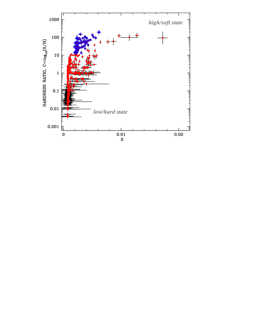
Figure 1: Color-intensity evolutionary diagram for M101 ULX-1 using $Swift$ observations (2006 –2012), where S and H are the source counts in the two bands: the $soft$ [0.3 – 1.5 keV] and $hard$ [1.5 – 10 keV] passbands. Spectral softness (hardness ratio) C and source soft brightness $S$ increase to the right and finally the former one saturates at high values of S. Larger values of $C$ indicate a softer spectrum, and vice versa. $Blue$ points are related to a decay part of the outburst (see the light curve in Fig. 4.

As for the distance estimate for M101 ULX-1, Kelson et al. (1996) provide a value of 7.4 Mpc while Freedman et al. (2001) argue that the distance is less and it is about 6.8 Mpc. Recently, Shappe & Stanek (2011) obtained a Cepheid distance to M101 using archival HST/ACS time series photometry of the $inner$ fields of the galaxy based on a larger Cepheid sample. They improved the distance determination for M101 and obtained a distance value of $d_{m101}=6.4\pm$0.5 Mpc.

In this Paper we present an analysis of available Swift and $Chandra$ observations of M101 ULX-1. In §2 we present the list of observations used in the data analysis while in §3 we provide details of the X-ray spectral analysis. We discuss the evolution of the X-ray spectral properties during the high-low state transition and present the results of the scaling analysis to estimate BH mass of M101 ULX-1 in §4. We make our final conclusions in §5.

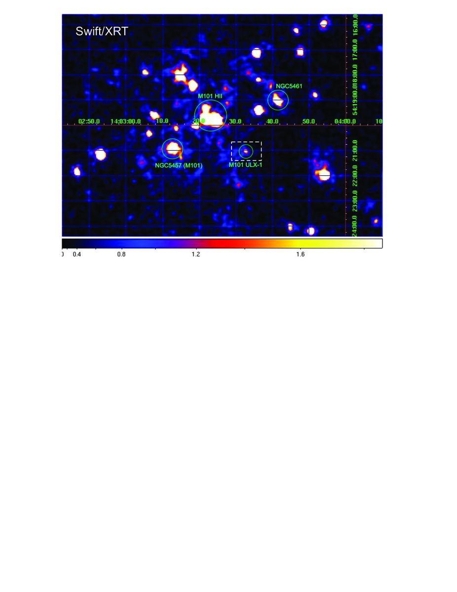
Figure 2: $Swift$/XRT (0.3$-$10 keV) image of M101 field of view, where green circles are the locations of M101 ULX-1, M101 galactic nucleus (NGC 5457), NGC 5461 and M101 H II regions. The image segment selected by dashed line box is also shown in Fig. 3 using $Chandra$ data.

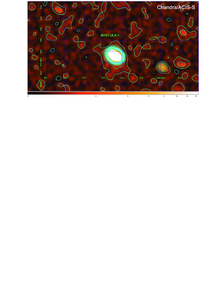
Figure 3: Adaptively smoothed $Chandra$/ACIS-S (0.2-8 keV) image of the M101 field, which localization is indicated by the selected dashed line box in Fig. 2. Contour levels demonstrate the minimal contamination by other point sources and diffuse emission within circle of 9" around M101 ULX-1.

2 Observations and data reduction

As the first step we analyzed the Swift data set for M101 ULX-1, which covered the longest observational interval (2006 – 2013). In this way, we studied the source behavior in X-rays (Sect. 2.1).  Then we proceeded with a detailed spectral analysis using the Chandra (2000, 2004 – 2005) data (§ 2.2). A summary of the X-ray observations considered in this work is given in Tables 1 and 2.

Table 1: The list of $Swift$ observations of M101 ULX-1 used in our analysis

Obs. ID	Start time (UT)		End time (UT)	MJD interval
00035892001	2006 Aug. 29 11:38:56		2006 Aug. 29 21:24:57	53976.8 – 53976.9
00030896(001-009)	2007 March 1		2007 Apr. 19	54160 – 54209
00032081(001-149)	2011 Aug. 24		2012 May 10	55797 – 56058
00032094(001-018)	2011 Sep. 7		2013 Sep. 11	55811 – 56546
00032101(001-013)	2011 Sep. 23		2013 Sep. 20	55827 – 56555
00032481001	2012 June 9 10:17:15		2012 June 9 13:55:57	56087.4 – 56087.5

2.1 Swift data

The log of the Swift/XRT observations used in this Paper is shown in Table 1. The Swift source count rates never exceed 0.02 count s^-1, therefore only photon-counting mode (PC) events (selected in grades 0$-$12) were considered. In this way, the $Swift$-XRT/PC data (ObsIDs, indicated in the first column of Table 1) were processed using the HEA-SOFT v6.14, the tool XRTPIPELINE v0.12.84 and the calibration files (CALDB version 4.1). The ancillary response files were created using XRTMKARF v0.6.0 and exposure maps generated by XRTEXPOMAP v0.2.7. We fitted the spectrum using the response file SWXPC0TO12S6$\_$20010101v012.RMF. We also used the online XRT data product generator for independent check: light curves and spectra (including background and ancillary response files, see Evans et al. 2007, 2009). We have made the state identification in terms of the color ratio (see Sect. 3.2), using the Bayesian method developed by Park et al. (2006). Moreover, we have applied the effective area option of the Park’s code which includes the count-rate correction factors in their calculations. Our results, adapting this technique, indicate to two color$-$intensity regimes in M101 ULX-1: i. with low color ratio at lower count-rate observations and ii. high color ratio at higher count events (see Figure 1). Furthermore the color$-$intensity diagram shows a smooth track. Therefore, we have grouped the $Swift$ spectra into four bands according to count rates (see Sect. 3.1) and fitted the combined spectra of each band using the XSPEC package (version 12.8.14).

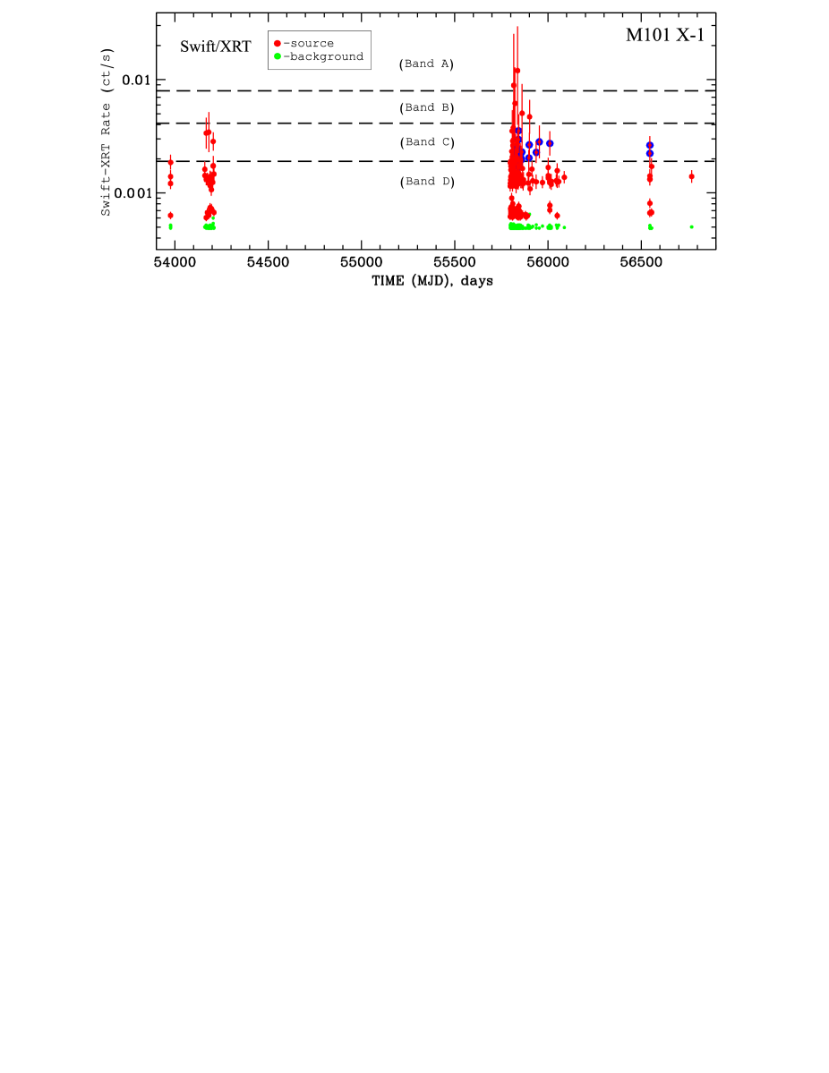
Figure 4: $Swift$/XRT light curve of M101 ULX-1 in the 0.3$-$10 keV band during 2006 – 2013. $Red$ points mark the source signal and $green$ points indicate the background level. $Blue$ points mark decay part of the outburst for this light curve and correspond to $blue$ points of color-intensity evolutionary diagram (see higher branch) shown in Fig. 1.

Table 2: The list of $Chandra$ observations of M101 ULX-1

Obs. ID	Start time (UT)	Rem.	Obs. ID	Start time (UT)	Rem.	Obs. ID	Start time (UT)	Rem.
9341,2,3,4	2000-03-26	HS	53221,3	2004-05-03	LS	47341,3	2004-07-11	HS
20651,2,3	2000-10-29	HS	47331,3	2004-05-07	LS	47361	2004-11-01	LS
47311,3	2004-01-19	LS	53231,3	2004-05-09	LS	61521	2004-11-07	LS
52971,3	2004-01-24	LS	53371,3	2004-07-05	HS	61701,2	2004-12-22	LS
53001,3	2004-03-07	LS	53381,3	2004-07-06	HS	61751,2	2004-12-24	LS
53091,3	2004-03-14	LS	53391,3	2004-07-07	HS	61691,2	2004-12-30	HS
47321,3	2004-03-19	LS	53401,3	2004-07-08	HS	47371,2	2005-01-01	HS

(1) Mukai et al. 2005; (2) Kong & Di Stefano 2005; (3) Kong et al. 2004; (4) Pence et al. 2001.

2.2 Chandra data

M101 ULX-1 was also observed by Chandra in 2000, 2004$-$2005. The log of Chandra observations used in this Paper is presented in Table 2. We extracted spectra from the ACIS-S detector using the standard pipeline CIAO v4.5 package and calibration database CALDB 2.27. All data were taken in very faint mode (VFAINT) except for the data taken in 2000, March 26 and October 29, which were used in faint mode (FAINT). We have also identified intervals of high background level in order to exclude all high background events. The Chandra spectra were produced and modelled over the 0.3 – 7.0 keV energy range. Note that the data during the low state (indicated by * in Table 2), are characterized by only a few photons ($\sim$10 – 30) for each observation. Therefore, we combined all the low state data to perform statistically significant spectral fits. Thus, we present the results for these low state data per observation using C-statistic. While the rest of the data are analyzed in terms of $\chi^{2}$-statistics.

3 Results

3.1 Images

In order to avoid a possible contamination from nearby sources we made a visual inspection of the obtained image (smoothed by a Gaussian with an FWHM of 3"2). Swift/XRT (0.3 – 10 keV) image of M101 field of view is presented in Figure 2, where green circles are the locations of M101 ULX-1, NGC 5457 (M101), NGC 5461 and M101 H II regions.

For deeper image analysis we used the Chandra images with better data quality, provided by ACIS-S onboard Chandra. We point out the Chandra region as shown by dashed line box in the Swift image in Figure 2. The Chandra/ACIS-S (0.2-8 keV) image obtained during observations of M101 ULX-1 on March 26, 2000 (with exposure time of 99.5 ks, ObsID=934) is diplayed in Figure 3. Contour levels should demonstrate the minimal contamination by other point sources and diffuse emission within circle of 9 arsec around M101 ULX-1. For each observation, we extracted the source spectrum from a 9" radius circular region centered on the source position of M101 ULX-1 [$\alpha=14^{h}03^{m}32^{s}.37$, $\delta=54^{\circ}21{\tt{}^{\prime}}02{\tt{}^{\prime\prime}}.7$, J2000.0, see details in Kuntz et al. (2005)], while an annulus region centered on the source with 10 and 18" radii was used to estimate the background contribution.

In addition, we extracted emission related to the other bright nuclear sources NGC 5457, NGC 5461 from circular regions with radius of 15" and retrace their time behavior. As a result we established that only M101 ULX-1 demonstrated significant variability during the analyzed observations.

3.2 Color-intensity diagrams and light curves

Before detailed detailed spectral fitting we investigated a so called color ratio to quantify and characterize the source spectrum. In particular, for our $Swift$ data we consider $R$ as a ratio of the counts $S$ and $H$ in the soft (0.3 – 1.5 keV) and hard (1.5 – 10 keV) bands, respectively. However, at low counts, the posterior distribution of the counts ratio, $R$, tends to be skewed because of the Poissonian nature of data. Therefore we used the color, $C=log_{10}(S/H)$, which a log transformation of $R$, which provides the skewed distribution more symmetric (see e.g., Park et al. 2006). The ratio $C$ is modified by taking into account background counts and instrumental effective areas. Figure 1 demonstrates the color-intensity diagram and thus one can see that different count-rate observations correspond to different color regimes. Larger values of $C$ indicate a softer spectrum, and vice versa. Note that we have applied a Bayesian approach to compute the ratio values $C$ and their errors using BEHRs software  (Park et al., 2006). Generally, this method is applicable when the source is faint or the background is relatively large (Evans et al., 2009; Burke et al., 2013; Jin et al., 2006). In our case, the most $Swift$ observations are related to low count-rate regimes, which can confuse a reliable color estimates. However, Bayesian analysis provides a simple way to overcome this problem. As a result, we found a clear LS-HS evolution of X-ray emission from M101 ULX-1. Furthermore, Figure 1 demonstrates that the color $C$ monotonically increases with the soft flux $S$ and achieves a noticeable stability at high soft fluxes. Note that the color-color diagram of M101 ULX-1 clearly demonstrates two groups of datapoints, related to the high/soft and low/hard states (see Fig. 1). More specifically, in outbursts, M101 ULX-1 evolves from the $hard$ state to the $soft$ state during the rise phase and then returned to the $hard$ state during the decay phase. This evolution is similar to most outbursts of Galactic X-ray binary transients (e.g. Homan et al. 2001; Shaposhnikov & Titarchuk, 2006; Belloni et al. 2006; ST09; TS09; Shrader et al. 2010; Mu$\tilde{n}$oz-Darias et al. 2014).

The source M101 ULX-1 is in the low state (characterized by a low count rate) during most of the time except for relatively short outbursts (with a high count rate, see Fig. 4 for details). Because of a low count rate we combined all of the low state data for Chandra and Swift data.

In Figure 4 we present Swift/XRT light curve of M101 ULX-1 during 2006 – 2013 for the 0.3 – 10 keV band. Red points mark the source signal and $green$ points indicate the background level. We have detected an outburst of M101 ULX-1 at MJD=55800 – 56100, while for the rest of the Swift observations this source remained in the low state. Individual Swift/XRT observations of M101 ULX-1 in PC (Photon counting) mode do not have enough counts to allow statistically meaningful spectral fits. To overcome this problem, we have examined the Swift/XRT lightcurve and grouped the observations into four bands: very high (”A”), high (”B”), medium (”C”) and low (”D”) count rates (see Fig. 4). We have also split Band C into two subbands. Blue points shown in Figure 1 are associated with softer/higher track (see also related points in the lightcurve, Fig. 4). In fact, this softer track ($blue$ points of Figure 1) corresponds to the outburst decay part (see Fig. 4). While Band-C_h (red points) are related to the lower track of the color-intensity diagram. Finally, we have combined the spectra in each related band and fitted them for all these observations using $\chi^{2}$ statistics. In addition, some of the brightest source spectra of A- and B-sets were regrouped with the task grppha and then analysed in the 0.3 – 7 keV range using the Cash statistics.

3.3 Spectral Analysis

We examine different spectral models in application to all available data for M101 ULX-1 in order to describe the source evolution between the $low$ and $hard$ states. Specifically, we use the combined $Swift$ spectra from different spectral states to test a number of spectral models: $powerlaw$, $Bbody$, $bmc$ and their possible combinations modified by an absorption model. We fitted all spectra using a tied neutral column, which provides the best-fit column $N_{H}$ of $3\times 10^{21}$ cm^-2.

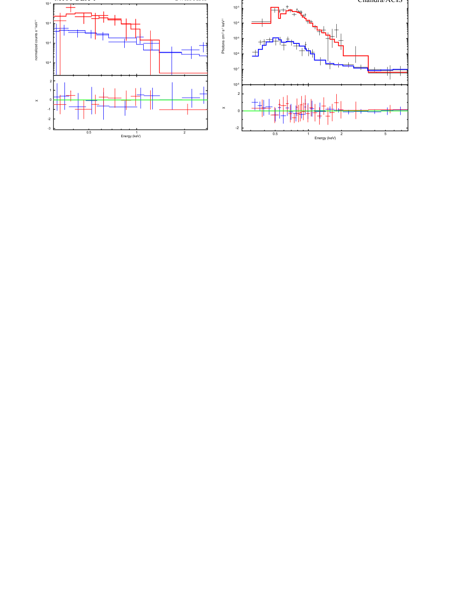
Figure 5: ($Left$:) $Swift$/XRT spectra from band A ($red$) and band C ($blue$) fitted using the $bmc$ model. ($Right$:) two representative $Chandra$ spectra for different states of M101 ULX-1. Data taken for 2004 July 5 ($red$), correspond to the high state spectrum and for 2004 January – May and November ($blue$), correspond to the low state spectrum. Spectra are fitted by a $phabs*bmc$ model with $kT_{bb}=70$ eV (red solid line), for the high state and with $kT_{bb}=45$ eV (blue solid line), for the low state. See also the best-fit parameters listed in Tables 3 and 4 for $Swift$ and $Chandra$ data, respectively.

Table 3: Best-fit parameters of the combined $Swift$ spectra of M101 ULX-1 in the 0.3$-$7 keV energy range using the following four models^†: $phabs*power$, $phabs*bbody$, $phabs*(bbody+power)$ and $phabs*bmc$

Model	Parameter	Band-A	Band-B	Band-Ch	Band-Cs	Band-D
Power-law	$\Gamma_{pow}$	6.2$\pm$0.2	3.6$\pm$0.3	1.9$\pm$0.2	2.0$\pm$0.2	1.4$\pm$0.2
	N${}_{pow}^{\dagger\dagger}$	2.8$\pm$0.03	1.4$\pm$0.02	0.67$\pm$0.05	0.68$\pm$0.04	0.04$\pm$0.01
	$\chi^{2}$ (d.o.f.)	2.3 (18)	2.15 (18)	2.03 (18)	2.02 (18)	1.15 (18)
Bbody	TBB	65$\pm$2	70$\pm$3	85$\pm$3	84$\pm$5	94$\pm$4
	N${}_{BB}^{\dagger\dagger}$	5.2$\pm$0.5	4.5$\pm$0.3	2.7$\pm$0.6	2.8$\pm$0.5	1.5$\pm$0.4
	$\chi^{2}$ (d.o.f.)	1.14 (18)	1.28 (18)	1.94 (18)	1.93 (18)	3.03 (18)
Bbody	TBB	70$\pm$3	86$\pm$4	90$\pm$5	89$\pm$3	70$\pm$4
	N${}_{BB}^{\dagger\dagger}$	4.2$\pm$0.5	3.6$\pm$0.6	1.4$\pm$0.6	1.6$\pm$0.5	1.3$\pm$0.4
Power-law	$\Gamma_{pow}$	2.2$\pm$0.1	2.1$\pm$0.4	1.4$\pm$0.1	1.5$\pm$0.1	3.4$\pm$0.3
	N${}_{pow}^{\dagger\dagger}$	0.64$\pm$0.01	0.57$\pm$0.03	0.36$\pm$0.09	0.38$\pm$0.07	1.3$\pm$0.4
	$\chi^{2}$ (d.o.f.)	1.23 (16)	1.19 (16)	1.23 (16)	1.22 (16)	1.27 (16)
bmc	$\Gamma_{bmc}$	2.5$\pm$0.3	2.1$\pm$0.2	1.6$\pm$0.1	1.7$\pm$0.1	1.4$\pm$0.1
	Ts	92$\pm$10	76$\pm$9	56$\pm$10	57$\pm$10	42$\pm$8
	logA	-5.3$\pm$0.4	-4.7$\pm$0.5	-4.3$\pm$0.4	-4.2$\pm$0.5	-3.9$\pm$0.5
	N${}_{bmc}^{\dagger\dagger}$	15.6$\pm$0.5	8.1$\pm$0.3	4.4$\pm$0.2	4.5$\pm$0.4	2.9$\pm$0.2
	$\chi^{2}$ (d.o.f.)	1.21 (16)	0.97 (16)	1.15 (16)	1.14 (16)	1.03 (16)

3.3.1 Choice of the Spectral Model

As a first step, we proceed with a model of an absorbed power-law. This model ($phabs*powerlaw$) fits well the low state data only [e.g., for D-spectra, $\chi^{2}_{red}$=1.15 (18 d.o.f.), see the left column of Table 3]. As one can see the power-law model is characterized by very large photon indices (much greater than 3, particularly for A and B-event spectra, see notations of these events in Fig. 4) and furthermore, this model gives unacceptable fits (e.g., for all A, B and C-spectra of $Swift$ data). On the other hand, for the $high$ state data, the thermal model ($Bbody$) provides better fits than the power-law model. However, the intermediate state spectra (B-, C-spectra for $Swift$ data) cannot be fitted by any single-component model. In particular, a simple power-law model produces a soft excess. Significant positive residuals at low energies less than 1 keV suggest the presence of additional emission components. For this reason, we also use a sum of blackbody and power-law component model ($N_{H}=3\times 10^{21}$ cm^-2, $kT_{bb}=70-90$ eV, and $\Gamma=1.4-2.2$; see Table 3). The best fits of $Swift$ spectra has been obtained by implementation of the so called Bulk Motion Comptonization model [BMC XSPEC model, Titarchuk et al. (1997)], for which the photon index ranges from $\Gamma\sim 1.4-2.8$ for all observations (see Tables 3, 4 and Fig. 5). Furthermore, we achieve the best-fit results using the same model for all spectral ($high$ and $low$) states.

We should remind a reader that the BMC model is characterized by the seed photon temperature $T_{s}$, the energy index of the Comptonization spectrum $\alpha$ ($\alpha=\Gamma-1$), the illumination parameter $\log(A)$ related to the Comptonized (illumination) fraction $f=A/(1+A)$. This model convolves a seed (disk) blackbody with an upscattering Green’s function. We also use a multiplicative $phabs$ component to take into account an absorption by neutral material. The $phabs$ model parameter is an equivalent hydrogen column $N_{H}$. In Table 3 we demonstrate a good performance of the BMC model in application to the $Swift$ data ($0.97<\chi^{2}_{red}<1.21$).

Table 4: Best-fit parameters of the spectra using $Chandra$ observations of M101 ULX-1 in the 0.3 – 7 keV energy range^†. Parameter errors correspond to 90% confidence level.

ObsID	MJD, day	Exp, ks	Counts	$kT_{s},$ keV	$\Gamma_{bmc}=\alpha_{bmc}+1$	$\log{A}$	N${}_{bmc}^{\dagger\dagger}$	$\chi^{2}_{red}$ (d.o.f.), MC†††
934	51629	94	8642	100$\pm$21	2.78$\pm$0.08	-3.78(9)	35.2(3)	0.99 (28)
2065	51846	10	310	67$\pm$10	2.6$\pm$0.1	-2.36(8)	18.9(1)	1.08 (10)
4731*	53023	56	26	46$\pm$10	1.39$\pm$0.07	-2.1(5)	2.2(1)	0.89
5297*	53028	15	14	42$\pm$9	1.38$\pm$0.04	-2.0(6)	2.3(2)	0.78
5300*	53071	52	13	43$\pm$8	1.38$\pm$0.05	-2.0(6)	2.2(1)	0.99
5309*	53078	71	18	44$\pm$9	1.37$\pm$0.06	-2.0(5)	2.1(1)	0.98
4732*	53083	70	12	42$\pm$8	1.38$\pm$0.04	-2.0(3)	2.1(1)	0.91
5322*	53128	65	17	45$\pm$10	1.39$\pm$0.08	-2.0(5)	2.2(1)	0.93
4733*	53132	16	12	41$\pm$7	1.36$\pm$0.07	-2.0(4)	2.1(1)	0.85
5323*	53134	43	10	40$\pm$10	1.35$\pm$0.09	-2.5(2)	2.0(1)	0.82
5337	53191	10	129	70$\pm$12	1.65$\pm$0.09	-3.32(9)	4.6(2)	0.97 (12)
5338	53192	28	162	98$\pm$25	1.89$\pm$0.07	-2.93(8)	6.3(1)	1.00 (30)
5339	53193	14	468	65$\pm$14	1.97$\pm$0.1	-4.18(6)	6.9(1)	1.08 (20)
5340	53194	54	680	51$\pm$3	2.72$\pm$0.09	-2.4(3)	30.6(3)	1.21 (23)
4734	53197	35	582	60$\pm$9	2.12$\pm$0.06	-3.9(4)	8.7(1)	1.25 (14)
4736*	53310	78	29	45$\pm$8	1.36$\pm$0.07	-2.4(2)	2.0(1)	0.89
6152*	53316	44	21	43$\pm$9	1.36$\pm$0.08	-2.4(3)	2.1(2)	0.96
6170	53361	48	41	47$\pm$12	1.5$\pm$0.1	-2.0(1)	3.1(5)	0.6 (5)
6175	53363	41	54	45$\pm$10	1.9$\pm$0.3	-3.7(1)	5.7(1)	0.78 (6)
6169	53369	29	613	71$\pm$5	2.1$\pm$0.1	-4.1(2)	8.1(1)	1.12 (20)
4737	53371	20	1483	95$\pm$7	2.75$\pm$0.06	-3.9(1)	26.7(1)	1.08 (54)
Comb.LS**	…	500	172	45$\pm$10	1.39$\pm$0.08	-2.0(5)	2.2(1)	0.93 (10)

3.3.2 Bulk Motion Comptonization model and its application to M101 ULX-1

The Bulk Motion Comptonization (BMC) model has successfully fitted the M101 ULX-1 spectra for all spectral states. Specifically, $Swift$/XRT spectra for band A ($red$) and band C ($blue$) fitted using the BMC model are presented in Figure 5 ($left$ panel). The plot highlights the significant spectral variability between these sets of the observations (see Figure 4 for our definition of $Swift$/XRT count-rate bands, and Table 3 for the best-fit parameters). In Table 3 (at the bottom), we present the results of spectral fitting $Swift$/XRT data of M101 ULX-1 using the $phabs*bmc$ model. In particular, the LS$-$HS transition is related to the photon index $\Gamma$ change from 1.4 to 2.5 when the relatively low seed photon temperature $kT_{s}$ changes from 40 eV to 90 eV. Note the $bmc$ normalization varies by factor five, namely in the range of $2.9<N_{BMC}<15.6\times L_{35}/d^{2}_{10}$ erg s^-1 kpc^-2. While the Comptonized (illumination) fraction is quite low ($\log{A}<-4$ or $f\sim 10^{-4}$) for all cases.

As we have already pointed out above, Pence et al. (2001), Mukai et al. (2005), Kong et al. (2004) and Kong & Di Stefano (2005) analyzing the $Chandra$ data investigated the spectral evolution of M101 ULX-1. We have also found a similar spectral behavior for the selected data set (see Table 2) using our model. In particular, we have revealed that M101 ULX-1 was in the high state during three outbursts: at 2000 (March and October); at 2004 July and at 2004 December 30 – 2005 January 1. The other $Chandra$ observations are related to the low state when the source is seen at the detection limit. The low state events of M101 ULX-1 covers long time intervals: during 2004 January, March, May, November and December. Usually in the low state the X-ray luminosity of ULX-1 is about a factor 100 lower than that during the high state, when the peak bolometric luminosity (for assumed isotropic emission) is about $10^{41}$ ergs s^-1.

In the $right$ panel of Figure 5 we demonstrate two representative $Chandra$ spectra for different states of M101 ULX-1. Data taken for 2004 July 5 ($red$), which correspond to the high state spectrum and for 2004 January – May and November ($blue$) which correspond to the low state spectrum. These spectra have been fitted by a $phabs*bmc$ model with the best fit parameters $kT_{s}=70$ eV ($red$ solid line, for the high state) (HS) and $kT_{s}=45$ eV ($blue$ solid line, for the low state) (LS). We list the best-fit spectral parameters in Table 4. The shapes of these spectra related to these two states, are different. In the LS state the seed photons (with the lower $kT_{s}$ presumably related to lower mass accretion rate) are Comptonized more efficiently because the illumination fraction $f$ [or $\log(A)$] is higher. On the other hand in the HS state, these parameters, $kT_{s}$ and $\log(A)$ show an opposite behavior, namely $\log(A)$ is lower for higher $kT_{s}$. That means that a relatively small fraction of the seed photons, which temperature is higher because of the higher mass accretion rate in the HS than that in the LS, is Comptonized.

We also evaluated the blackbody radius $R_{BB}$ derived using a relation $L_{BB}=4\pi R^{2}_{BB}\sigma T^{4}_{BB}$, where $L_{BB}$ is the luminosity of the blackbody and $\sigma$ is Stefan’s constant. Assuming a distance D of 7.6 Mpc (as an upper estimate), the region associated with the blackbody has the radius $R_{BB}\leq 3\times 10^{6}$ km, which clear indicates the IMBH presence in M101 ULX-1. In fact, $R_{BB}$ should be of order $10-30$ km for a Galactic BH of mass around 10 solar masses.

It is worth noting that our spectral model shows very good performance throughout all data sets. The reduced $\chi^{2}_{red}=\chi^{2}/N_{dof}$ (where $N_{dof}$ is the number of degree of freedom) is less or around 1.0 for the most of the observations. For a small fraction (less than 3%) of the spectra with high counting statistics $\chi^{2}_{red}$ reaches 1.4. However, it never exceeds a rejection limit of 1.5.

3.3.3 Evolution of X-ray spectral properties during spectral state transitions

We have established common characteristics of the HS and LS spectral transitions of M101 ULX-1 (as seen in Fig. 4) based on their spectral parameter evolution of X-ray emission in the energy range from 0.3 to 7 keV using $Swift$/XRT and $Chandra$/ACIS data. In Figures 4 we show the light curves highlighting the X-ray variability of the source. In Figure 6, from top to bottom we demonstrate an evolution of the seed photon temperature $kT_{s}$, the BMC normalization and the spectral index $\alpha=\Gamma-1$ during 2004$-$2005 outburst transitions observed with $Chandra$/ACIS-S. The outburst phases of the LS$-$HS transitions are marked by blue vertical strips.

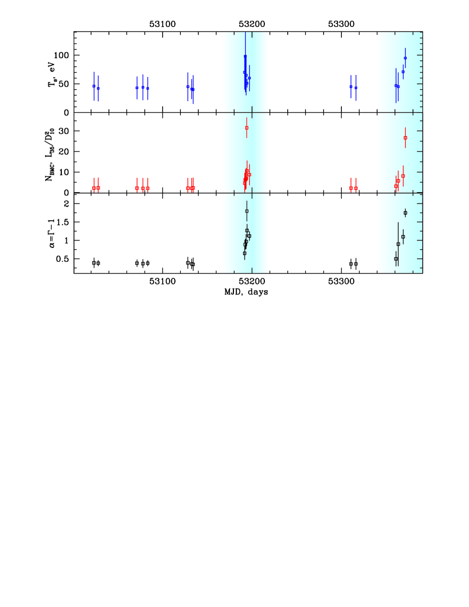
Figure 6: From Top to Bottom: Evolutions of the seed photon temperature $kT_{s}$ in eV, the $BMC$ normalization and the spectral index $\alpha=\Gamma-1$ during 2004$-$2005 outburst transitions observed with $Chandra$/ACIS-S. The outburst phases of the LS$-$HS transitions are marked by blue vertical strips.

During the rise phase and close to the peak of outburst, the softer emission [0.3$-$1 keV] dominates in the spectrum, which is associated with the seed photon temperatures $kT_{s}=40-60$ eV (see upper panel of Fig. 6). At the outburst we detected the maximum of the seed photon temperature $kT_{s}=100$ eV (see e.g. MJD=53194 point) along with the maximum of the normalization $N_{bmc}$. Through the next days after outburst, mass accretion rate $\dot{M}$ drops by about a factor of ten (the BMC normalization parameter $N_{bmc}\propto\dot{M}$), $kT_{s}$ again drops to 60 eV when the source comes back its “standard” low state. In turn, a long “standard” low state of M101 ULX-1 is associated with the low seed photon temperatures $kT_{s}=40$ eV (see e.g. MJD=53000 – 53150 interval in $T_{s}$-panel of Fig. 6) and the low Comptonized fraction $f$ (see also Tables 3$-$4).

From this plot we see that all spectral parameters correlate with each other during the LS$-$HS transitions. In particular, the correlations of the photon index $\Gamma$ ($=\alpha+1$) versus BMC normalization $N_{BMC}$ are presented in Figure 7, where $blue$ triangles and $red$ squares are related to $Swift$ and $Chandra$ data, respectively. In Figure 7 we also show the photon index $\Gamma$ ($=\alpha+1$) monotonically increases from 1.3 to 2.8 with $N_{BMC}$ (proportional to $\dot{M}$) and saturates at $\Gamma_{sat}=2.8\pm 0.1$ for high values of $N_{BMC}$. One can see the strong saturation effect of the index $\Gamma$ versus $N_{BMC}$.

4 Discussion

Before proceeding with the interpretation of the observations, let us briefly summarize them as follows. (1) The spectral data of M101 ULX-1 are well fitted by the BMC model for all analyzed LS and HS spectra [see Figure 5 and Tables 3$-$4]. (2) The Green’s function index of the BMC component $\alpha$ (or the photon index $\Gamma=\alpha+1$) rises and saturates with an increase of the BMC normalization (proportional to $\dot{M}$). The photon index saturation level of the BMC component is about 2.8 (see Figure 7).

4.1 Saturation of the index is a signature of a BH

Using our analysis of the evolution of $\Gamma$ in M101 ULX-1 we have firmly established that $\Gamma$ saturates with the BMC-normalization $N_{BMC}$, which is proportional to $\dot{M}$. ST09 give strong arguments that this $\Gamma$ saturation is a signature of converging flow into a BH.

Titarchuk et al. (1998) predicted that the transition layer (TL), the sub-Keplerian part of the accretion flow, should become more compact when $\dot{M}$ increases. For a BH case, Titarchuk & Zannias (2008), hereafter TZ98, obtain semi-analytically and later Laurent & Titarchuk (1999), (2011), hereafter LT99 and LT11, find, using Monte Carlo simulations, that $\Gamma$ saturates for high mass accretion rates. Analyzing a number of Galactic BHs (GBHs) ST09, Titarchuk & Seifina (2009), Seifina & Titarchuk (2010) and Seifina et al. (2014) (STS14) confirm the LT99-11 prediction that $\Gamma$ increases and then it saturates with $\dot{M}$. In Figure 7 one can see that the values of $\Gamma$ monotonically increase from 1.3 and then they finally saturate at a value of 2.8 for this particular source ULX-1 in M101.

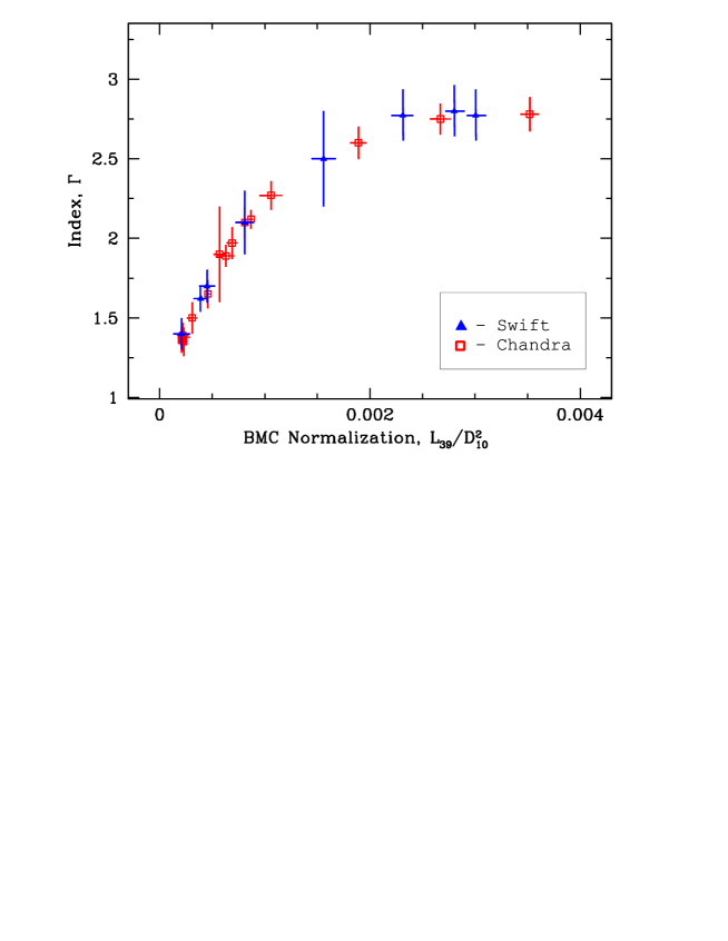
Figure 7: Correlations of the photon index $\Gamma$ ($=\alpha+1$) vs the BMC normalization $N_{BMC}$ (proportional to mass accretion rate) in units of $L_{39}/D^{2}_{10}$. $Blue$ triangles and $red$ squares are related to $Swift$ and $Chandra$ observations, respectively.

We observed the luminosity increase along with the intrinsic softening of the spectrum lasting about three days. When the luminosity drops, we find the spectral hardening as a decrease of $\Gamma$ in agreement with the theoretical expectations (see TZ98, LT99-11). This $\Gamma$ vs. $\dot{M}$ correlation found using the M101 ULX-1 spectra are probably driven by the same physical process that causes the spectral evolutions seen in X-ray binaries due to the change of $\dot{M}$. Moreover, we argue that the X-ray observations of M101 ULX-1 reveal the strong index saturation vs $\dot{M}$ as a signature of the converging flow (or BH presence) in this source (see ST09). The index-$N_{BMC}$ normalization (or $\dot{M}$) correlations found in a number of GBHs allow us to estimate a BH mass in M101 ULX-1 (see below §4.2).

Table 5: Parameterizations for reference and target sources

Reference source	A	B	D	$x_{tr}$	$\beta$
XTE J1550-564 RISE 1998	2.84$\pm$0.08	1.8$\pm$0.3	1.0	0.132$\pm$0.004	0.61$\pm$0.02
H 1743-322 RISE 2003	2.97$\pm$0.07	1.27$\pm$0.08	1.0	0.053$\pm$0.001	0.62$\pm$0.04
4U 1630-472	2.88$\pm$0.06	1.29$\pm$0.07	1.0	0.045$\pm$0.002	0.64$\pm$0.03
Target source	A	B	D	$x_{tr}[\times 10^{-4}]$	$\beta$
M101 ULX-1	2.88$\pm$0.06	1.29$\pm$0.07	1.0	4.2$\pm$0.2	0.61$\pm$0.03

4.2 Estimate of BH mass in M101 ULX-1

To scale the BH mass $M_{BH}$ of the target source (M101 ULX-1), we select appropriate Galactic reference sources [XTE J1550-564, H 1742-322 (see ST09) and 4U 1630-47 (STS14)] whose masses and distances are known (see Table 6), and also their BMC normalizations $N_{BMC}$. We can compare the index vs $N_{BMC}$ (proportional to $\dot{M}$) correlations for these sources with that of the target source M101 ULX-1 (see Fig. 8). Note that for all these sources the index saturation level is at the almost same value of $\Gamma$. We have used these three reference sources for an additional cross-check of the BH mass evaluation of M101 ULX-1.

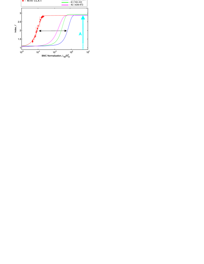
Figure 8: Scaling of the photon index $\Gamma$ versus the normalization $N_{BMC}$ for M101 ULX-1 (with $red$ points – target source) and 4U 1630-472, XTE J1550-564 and H1743-322 (with $pink$, $blue$ and $green$ mark the reference sources), respectively. The bright blue vertical arrow schematically shows that the parameter A is the value of the index saturation level. The horizontal black arrow stresses the fact that the correlations of the target and reference sources are similar. The only difference is in terms of the BMC normalization, due to the different values of the $M_{BH}/D^{2}$ ratio.

All correlation patterns are self-similar, showing the same index saturation level, which allows us to perform a reliable scaling. The BH mass scaling technique is generally based on the parameterization of the $\Gamma-N_{BMC}$ correlation, that according to ST09 is fitted by a function

$$F(x)=A-(D\cdot B)\ln\{\exp[(1.0-(x/x_{tr})^{\beta}))/D]+1\}.$$ (1)

where $x=N_{BMC}$.

By fitting this function to the correlation pattern, we find a set of parameters A, B, D, $N_{tr}$, and $\beta$ that represent a best-fit form of the function $F(x)$ for a particular correlation curve. For $x\gg x_{tr}$, the correlation function F(x) converges to a constant value A. Thus, A is the value of the index saturation level, $\beta$ is the power-law index of the inclined part of the curve and $x_{tr}$ is a value at which index $\Gamma$ starts growing and $\beta$ provides the slope of the correlation. A parameter $D$ determines how smoothly the fitted function saturates to A. This function $F(x$) is widely used for a description of the correlation of $\Gamma$ vs $N_{BMC}$ [Sobolewska & Papadakis (2009), ST09, Seifina & Titarchuk (2010), Shrader et al. (2010), STS14 and Giacche et al. (2014)].

The crucial assumption for this technique to be applied is that different reference sources show the same shape of the $\Gamma-N_{BMC}$ correlations and the only difference is in the ratio of a BH mass to the squared distance, namely in the coefficient $M_{BH}/d^{2}$. Figure  8 shows that a value of the parameter A (see bright blue vertical arrow) is almost the same for all scaling sources. In other words, the best-fit parameter $A$ (within the limits of error bars) is almost the same for all these sources. In particular, $A_{ULX}=2.8\pm 0.1$, $A_{1550}=2.84\pm 0.08$ and $A_{1743}=2.97\pm 0.07$ for M101 ULX-1, XTE J1550-564 and H 1743-322 respectively. Furthermore, the black horizontal arrow stresses that the correlations for a pair of sources [e.g., M101 ULX-1 ($red$ line) and XTE J1550-564 ($blue$ line)] are self-similar and the only difference is in the BMC normalization because of the different values of the $M_{BH}/D^{2}$ ratio.

Thus, in order to obtain the BH mass of M101 ULX-1, one should shift along $N_{BMC}-$axis the related correlation of the reference source to the one of the target source (see Fig. 8). This scaling technique provides a target BH mass value $M_{t}$:

$$M_{t}=M_{r}\frac{N_{t}}{N_{r}}\left(\frac{d_{t}}{d_{r}}\right)^{2}f_{G},$$ (2)

where t denotes the target, r stands for the reference and the geometric factor, by definition, $f_{G}=(\cos\theta)_{r}/(\cos\theta)_{t}$, the inclination angles $\theta_{r}$, $\theta_{t}$ and $d_{r}$, $d_{t}$ are distances to the reference and target sources respectively (see details in ST09). Note that the geometrical factor $f_{G}$ has to be considered when the accretion process is assumed to occur in disk-like geometry, while it is close to 1 in case of spherical accretion. Despite this uncertainty in the determination of $f_{G}$, we adopt the above formula for $f_{G}$ in which $\theta\sim i$ if information on the system inclination angle $i$ is available (see Table 6).

In Figure 8 we plot the $\Gamma-N_{BMC}$ for M101 ULX-1 points extracted using $Chandra$ and $Swift$ spectra along with those for the three reference patterns [4U 1630-47 ($pink$), XTE J1550-564 ($blue$), H 1743-322 ($green$)] which are similar to the correlation found for the target source. Scaling parameters for each of these pairs are presented in Table 6.

The target mass for M101 ULX-1 can be estimated using the relation

$$M_{t}=C_{0}{N_{t}}{d_{t}}^{2}f_{G}$$ (3)

where $C_{0}=(1/d_{r}^{2})(M_{r}/N_{r})$ is the scaling coefficient for each scaling pair (target and reference sources), masses $M_{t}$ and $M_{r}$ are in solar units and $d_{r}$ is the distance to a particular reference source measured in kpc.

We take values of $M_{r}$, $M_{t}$, $d_{r}$, $d_{t}$, and $\cos(i)$ from Table 6 and then we obtain the lowest limit of the mass, using the best fit value of $N_{t}=(4.2\pm 0.2)\times 10^{-4}$ taken at the begining of the index saturation (see Fig. 8) and measured in units of $L_{39}/D^{2}_{10}$ erg s^-1 kpc^-2 [see Table 5 for values of the parameters of function $f(N_{t})$ (Eq. 1)]. We estimate $C_{0}\sim 1.9,\leavevmode\nobreak\ 1.72\leavevmode\nobreak\ 1,83$ for XTE J1550-564, H 1723-322 and 4U 1630-472 respectively using $d_{r}$, $M_{r}$, $N_{r}$ presented by ST09. Then, using formula (3), we obtain that $M_{ULX}\geq 3.4\times 10^{4}\leavevmode\nobreak\ M_{\odot}$ ($M_{ULX}=M_{t}$), assuming $d_{ULX}\sim 6.4$ Mpc (Shappee & Stanek, 2011) and $f_{G}\sim 1$ (inclinations for both objects are the same). To take account of the spread in the distance to M101, we have made the same estimates of $M_{ULX}$ assuming $d_{ULX}=7.4\pm 0.6$ Mpc (Kelson et al., 2011) and derived higher values $M_{ULX}$ $\geq 4.3\times 10^{4}\leavevmode\nobreak\ M_{\odot}$. All these results are summarized in Table 6.

It is evident that the inclination of M101 ULX-1 system may be different from the inclination for the reference sources ($i\sim 60-70^{\circ}$), therefore we take this BH mass estimate for M101 ULX-1 as a lowest BH mass value because that $M_{ULX}$ is reciprocal function of $\cos(i_{ULX})$ [see Eq. 3 taking into account that $f_{G}=(\cos\theta)_{r}/(\cos\theta)_{t}$ there].

The obtained BH mass estimate is in agreement with a high bolometrical luminosity for M101 ULX-1 and $kT_{s}$ value which is in the range of 40$-$100 eV. In fact, a very soft spectrum is consistent with the relatively cold disk for ULXs that has also been considered as evidence for IMBHs (Miller et al. 2003, 2004; Wang et al. 2004).

It is also important to note that Kong et al. (2004), based on the comparison between the observed temperature ($kT\leq 100$ eV) and bolometric luminosity ($L_{bol}\sim 10^{40-41}$ ergs s^-1) during the 2004 July outburst, obtained a similar estimate on BH mass of M101 ULX-1. In fact, they obtained that BH mass in M101 ULX-1, $M_{m101}$ is greater than 2800 $M_{\odot}$. Furthermore, Kong & Di Stefano (2005) using the 90% lower limits of the disk blackbody fits derived from the 2004 December outburst, estimated $M_{m101}$ being in the range of $1.3\times 10^{3}-3\times 10^{4}M_{\odot}$.

Table 6: BH masses and distances.

Source	M${}^{a}_{dyn}$ (M${}_{\odot})$	i${}_{orb}^{a}$ (deg)	db (kpc)	Mscal (M⊙)
XTE J1550-5641,2,3	9.5$\pm$1.1	72$\pm$5	$\sim$6	10.7$\pm$1.5c
H 1743-3224	$\sim$11	$\sim$70	$\sim$10	13.3$\pm$3.2c
4U 1630–475	…	$\leq$70	$\sim$10 – 11	9.5$\pm$1.1
M101 ULX-16,7	3 – 1000	…	(6.4$\pm$0.5)$\times 10^{3}$	$\geq 3.2\times 10^{4}$
M101 ULX-17,8	3 – 1000	…	(7.4$\pm$0.6)$\times 10^{3}$	$\geq 4.3\times 10^{4}$

(1) Orosz et al. 2002; (2) S$\grave{a}$nchez-Fern$\grave{a}$ndez et al. 1999; (3) Sobczak et al. 1999; (4) McClintock et al. 2007; (5) STS14; (6) Shappee & Stanek 2011; (7) Mukai et al. 2005; (8) Kelson et al. 1996.

Liu et al. (2013) report on optical observations of M101 ULX-1 by Gemini/GMOS and they find that the system contains a Wolf-Rayet star with an orbital period of 8.2 days. The optical spectrum of the source is characterized by a broad helium emission line, including the He II 4686 Ȧ line. Because of the absence of a broad hydrogen emission line the authors argue that the star must be a Wolf-Rayet (WR). They propose the scenario that the intensities of the helium emission lines can be reproduced by the atmospheric model (see Hillier & Miller 1998) and the stellar mass is estimated to be 19 $M_{\odot}$ based on the empirical mass-luminosity relation (Schaerer & Maeder 1992 and Crowther 2007). Liu et al. find the mass function is about 0.18 $M_{\odot}$ for M101 ULX-1. Suggesting different values of inclination angle $i$ they propose that this BH mass is likely 20 – 30 $M_{\odot}$. In Figure 9 we present Liu’s BH estimate as a function of inclination angle $i$. The range of their BH mass estimates varies from 5 to 1000 solar masses depending on inclination angle $i$. For smaller $i$ a BH mass is higher (more than 1000 $M_{\odot}$) and for $i\leq 90^{\circ}$ it is about 5 solar masses.

Liu’s evaluation of the BH mass (20-30 $M_{\odot}$) is too low in comparison with our BH mass estimate and also it is in contradiction with the lower values of the soft seed photon temperature $kT_{s}$ (see discussion above). In fact, for a BH of 20-30 $M_{\odot}$ the seed temperature $kT_{s}$ is expected to be around 0.5 keV (see ST09). Liu et al. (2013) also point out that these low temperatures of the seed (disk) photons $kT_{s}\sim 70$ eV combined with high luminosities ($>10^{39}$ erg s^-1), which are observed in ULX-1 M101, complicate the interpretation of ULX-1 as a stellar-mass BH.

We derived the bolometric luminosity from the normalization of the BMC model between $7\times 10^{40}$ erg/s and $6\times 10^{41}$ erg/s (assuming isotropic radiation). This high luminosity is difficult to achieve in a X-ray binary unless the accretor has a mass greater than 1000 $M_{\odot}$. While our luminosity estimate is higher than that for previous M101 ULX-1 outbursts observed by XMM-$Newton$ in 2002 – 2005 but it is closer to that derived by Kong et al. (2004) (who used a combined power law plus $blackbody$ model). Note that on average $L_{x}$ luminosity is lower than the bolometrical one because the peak of the spectrum occurs at relatively low photon energies ($E\sim 0.1$ keV).

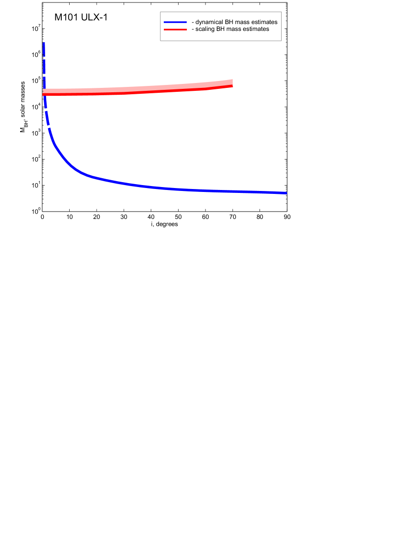
Figure 9: Estimates of BH mass $M_{BH}$ in M101 ULX-1. The $blue$ line represents $M_{BH}$ versus the inclination angle $i$ estimated using the dymanical method for HST data [taken from Liu et al. (2013)], while the $red$ line corresponds to our BH mass estimates based on X-ray data using the scaling technique (see Table 6). These two different methods give similar BH mass values with an assumption of small inclination angles.

5 Conclusions

We have studied the low$-$high state transitions observed in M101 ULX-1 using $Swift$ (2006 – 2013) and $Chandra$ (2000, 2004 – 2005) observations. We argued that the source spectra can be fitted by the BMC model for all observations. Our study reveals that the index$-$normalization (or $\dot{M}$) correlation observed in M101 ULX-1 is similar to those in GBHs. The photon index $\Gamma$ is in the range $\Gamma=1.3-2.8$. We have also estimated the peak bolometric luminosity, which is about $6\times 10^{41}$ erg s^-1.

We applied the scaling technique based on the observed correlations to estimate $M_{BH}$ in M101 ULX-1. This technique is commonly and successfully applied to estimate BH masses of Galactic black holes. In this work the scaling technique for the first time is applied to estimate $M_{BH}$ in ULX. We obtain values of $M_{BH}\sim(3.2-4.3)\times 10^{4}M_{\odot}$, which are in a good agreement with that estimated by peak bolometric luminosity estimates. The low limit of this BH mass estimate is in agreement with optical results (see Liu et al., 2013) assuming the face-on system configuration in ULX-1 (see Fig. 9). Combining these estimates with the inferred low temperatures of the seed disk photons $T_{s}$ we can state that the compact object of ultra-luminous source M101 ULX-1 is likely to be an intermediate-mass black hole with at least $M_{BH}>3.2\times 10^{4}M_{\odot}$.

- (1)
- Belloni et al. (2006) Belloni, T., Parolin, I., Del Santo, M., et al. 2006, MNRAS, 367, 1113
- Burke et al. (2013) Burke, M.J., Ralph P. Kraft, R.P., Soria, R. et al. 2013, ApJ, 775, 21
- Crowther (2007) Crowther, P.A. 2007, ARA&A, 45, 177
- Di Stefano & Kong (2003) Di Stefano, R., & Kong, A. K. H. 2003, ApJ, 592, 884
- Evans et al. (2009) Evans, P. A., Beardmore, A. P., Page, K. L., et al. 2009, MNRAS, 397, 1177
- Evans et al. (2007) Evans, P.A. et al. 2007, A&A, 469, 379
- Freedman et al. (2001) Freedman, W. L., et al. 2001, ApJ, 553, 47
- Giacche et al. (2014) Giacche, S., Gili, R. & Titarchuk, L. 2014, A&A, 562, A44
- Hiller & Miller (1998) Hiller, D. & Miller, D.L 1998, ApJ, 496, 407
- Homan et al. (2001) Homan, J., Wijnands, R., van der Klis, M., et al. 2001, ApJS, 132, 377
- Jin et al. (2006) Jin, Y. K., Zhang, S. N. & Wu, J. F. 2006, ApJ, 653, 1566
- Kelson et al. (2011) Kelson, D. D., et al. 1996, ApJ, 463, 26
- Kong et al. (2004) Kong, A. K. H., Di Stefano, R. & Yuan, F. 2004, ApJ, 617, L49
- Kong & Di Stefano (2005) Kong, A. K. H. & Di Stefano, R. 2005, ApJ, 632, L107
- Kuntz et al. (2005) Kuntz, K. D. et al. 2005, ApJ, 620, L31
- Laurent & Titarchuk (2011) Laurent, P., & Titarchuk, L. 2011, ApJ, 727, 34L
- Laurent & Titarchuk (1999) Laurent, P., & Titarchuk, L. 1999, ApJ, 511, 289 (LT99)
- Liu et al. (2013) Liu, J. et al. 2013, Nature, 503, 500
- Liu et al. (2012) Liu J. F., Orosz, J. & Bregman, J. N. 2012, ApJ, 745, 89
- Liu (2009) Liu, J. F. 2009, ApJ, 704, 1628
- Liu (2004) Liu, J. F., Bregman, J. N., Seitzer, P., Irwin, J. A. AAS Meeting 205, #104.03; Bulletin of the American Astronomical Society, Vol. 36, p.1515
- Mezcua et al. (2013) Mezcua, M., Farrell, S. A., Gladstone, J. C., Lobanov, A. P., 2013, MNRAS, 436, 1546
- McClintock et al. (2007) McClintock, J. E., Remillard, R. A., Rupen, M. P., Torres, M. A. P., Steeghs, D., Levine, A. M., & Orosz, J. A. 2007, ArXiv e-prints, 705, arXiv:0705.1034
- Miller et al. (2003) Miller, J. M., Fabbiano, G., Miller, M. C., & Fabian, A. C. 2003, ApJ, 585, L37
- Miller et al. (2004) Miller, J. M., Fabian, A. C., & Miller, M. C. 2004, ApJ, 614, L117
- Mukai et al. (2005) Mukai, K., Still, M., Corbet, R., Kuntz, K. & Barnard, R. 2005, ApJ, 634, 1085
- Mukai et al. (2003) Mukai, K., Pence, W. D., Snowden, S. L., Kuntz, K. D. 2003, ApJ, 582, 184
- Muoz-Darias et al. (2014) Muoz-Darias, T., Fender, R. P., Motta, S. E., & Belloni, T. M. 2014, MNRAS, 443, 3270
- Novikov & Thorne (1973) Novikov I. D., Thorne K. S., 1973, blho.conf, 343
- Orosz et al. (2002) Orosz, J. A. et al. 2002, ApJ, 568, 84
- Park et al. (2006) Park, T., Kashyap, V.L., Siemiginowska, A. et al. 2006, ApJ, 652, 610
- Pence et al. (2001) Pence, W. D., Snowden, S. L., Mukai, K., & Kuntz, K. D. 2001, ApJ, 561, 189
- Roberts et al. (2011) Roberts, T. P. et al., 2011 Astron. Nachr. 332, 398
- Roberts et al. (2008) Roberts, T. P., Levan, A. J. & Goad, M. R., MNRAS, 2008, 387, 73
- Sanchez-Fernandez et al. (1999) Sachez-Fernndez, C., et al. 1999, A&A, 348, L9
- Schaerer & Maeder (1992) Schaerer, D. & Maeder, A. 1992, A&A, 263, 129
- Shakura & Sunyaev (1973) Shakura, N. I., & Sunyaev, R. A. 1973, A&A, 24, 337
- Seifina et al. (2014) Seifina, E. & Titarchuk, L. & Shaposhnikov, N. 2014, ApJ, 789, 57 (STS14)
- Seifina & Titarchuk (2010) Seifina, E. & Titarchuk, L. 2010, ApJ, 722, 586 (ST10)
- Shaposhnikov & Titarchuk (2009) Shaposhnikov, N., & Titarchuk, L. 2009, ApJ, 699, 453 (ST09)
- Shaposhnikov & Titarchuk (2006) Shaposhnikov, N., & Titarchuk, L. 2006, ApJ, 643, 1098 (ST06)
- Shaposhnikov & Titarchuk (2004) Shaposhnikov, N., & Titarchuk, L. 2004, ApJ, 606, L57
- Shappee & Stanek (2011) Shappee, B. & Stanek, K. Z. 2011, ApJ, 733, 124
- Shrader et al. (2010) Shrader, Ch.R., Titarchuk, L. & Shaposhnikov, N. 2010, ApJ, 718, 488
- Sobczak et al. (1999) Sobczak, G. J., McClintock, J. E., Remillard, R. A., & Bailyn, C. D. 1999, ApJ, 520, 776
- Sobolewska & Papadakis (2009) Sobolewska M. A. & Papadakis, I.E. 2009, MNRAS, 399, 1997
- Titarchuk et al. (1997) Titarchuk, L. et al. 1997, ApJ, 487, 834
- Titarchuk et al. (1998) Titarchuk, L., Lapidus, I.I. & Muslimov, A. 1998, ApJ, 499, 315 (TLM98)
- Titarchuk (1994) Titarchuk, L. 1994, ApJ, 429, 340
- Titarchuk & Lyubarskij (1995) Titarchuk, L., & Lyubarskij, Y. 1995, ApJ, 450, 876
- Titarchuk & Seifina (2009) Titarchuk, L. & Seifina, E. 2009, ApJ, 706, 1463
- Titarchuk & Shaposhnikov (2005) Titarchuk, L. & Shaposhnikov, N. 2005, ApJ, 626, 298
- Titarchuk & Zannias (2008) Titarchuk, L. & Zannias, T. 2008, ApJ, 499, 315 (TZ98)
- Wang et al. (2004) Wang, Q. D., Yao, Y., Fukui, W., Zhang, S. N., & Williams, R. 2004, ApJ, 609, 113