A Holographic $c$-Theorem for Schrödinger Spacetimes

Abstract

We prove a $c$-theorem for holographic renormalization group flows in a Schrödinger spacetime that demonstrates that the effective radius $L(r)$ monotonically decreases from the UV to the IR, where $r$ is the bulk radial coordinate. This result assumes that the bulk matter satisfies the null energy condition, but holds regardless of the value of the critical exponent $z$. We also construct several numerical examples in a model where the Schrödinger background is realized by a massive vector coupled to a real scalar. The full Schrödinger group is realized when $z=2$, and in this case it is possible to construct solutions with constant effective $z(r)=2$ along the entire flow.

1 Introduction

In a relativistic conformal field theory, the Weyl anomaly $\langle T_{\mu}^{\mu}\rangle=\mathcal{A}$ signifies a breakdown of conformal invariance at the quantum level, and plays an important role in the characterization of the theory. This is especially true in two dimensions, where the Cardy formula relates the central charge $c$ to the degrees of freedom of the theory Cardy:1986ie . Moreover, the Zamolodchikov $c$-theorem demonstrates that it is possible to define a $c$-function that is monotonic decreasing along renormalization group flows from the UV to the IR Zamolodchikov:1986gt . These powerful statements have seen recent generalizations to four and higher dimensions as well DiPietro:2014bca ; Ardehali:2014zba ; Komargodski:2011vj .

From a relativistic AdS/CFT point of view, the leading holographic Weyl anomaly is easily obtained from the behavior of the on-shell action under rescaling of the boundary metric Henningson:1998gx . For example, for AdS_d+1, the leading contribution to the $a$ central charge is

$$a=\frac{2d\pi^{d/2}}{\kappa^{2}(d/2)!^{2}}L^{d-1},$$ (1)

where $L$ is the AdS radius and $\kappa$ is the gravitational coupling. While this is the result for pure, a holographic renormalization group flow may be realized geometrically by turning on a relevant deformation and then solving the equations of motion for radial evolution in the bulk. In particular, the AdS metric in the Poincaré patch

$$ds_{d+1}^{2}=e^{2r/L}(-dt^{2}+d\vec{x}_{d-1}^{2})+dr^{2},$$ (2)

has a natural domain wall generalization

$$ds_{d+1}^{2}=e^{2A(r)}(-dt^{2}+d\vec{x}_{d-1}^{2})+dr^{2}.$$ (3)

A flow between UV and IR fixed points is then given by the solution for $A(r)$ satisfying $A\sim r/L_{\rm UV}$ as $r\to\infty$ and $A\sim r/L_{\rm IR}$ as $r\to-\infty$. For such a flow, we may define an $a$-function by replacing the constant AdS radius $L$ in (1) by the effective radius $L(r)=1/A^{\prime}(r)$.

In this context, the holographic $c$-theorem Alvarez:1998wr ; Girardello:1998pd ; Freedman:1999gp ; Sahakian:1999bd states that the effective AdS radius $L(r)$ (and hence the $a$ function) is monotonic decreasing towards the IR. For Einstein gravity in the bulk, this follows directly from the null energy condition

$$R_{\mu\nu}l^{\mu}l^{\nu}=\kappa^{2}T_{\mu\nu}l^{\mu}l^{\nu}\geq 0,$$ (4)

for all future-directed null vectors $l^{\mu}$. In particular, choosing $l^{\mu}$ in the $t$–$r$ direction gives

$$R^{r}_{r}-R^{t}_{t}=-(d-1)A^{\prime\prime}\geq 0\qquad\Rightarrow\qquad L^{\prime}=-\frac{A^{\prime\prime}}{(A^{\prime})^{2}}\geq 0.$$ (5)

So long as we restrict to classical Einstein gravity in the bulk, the statement $L^{\prime}\geq 0$ is completely general (as long as we impose the null energy condition), and moreover holds in any spacetime dimension.

Given recent interest in non-relativistic holography, it is natural to ask whether a similar $c$-theorem can be shown in the context of Lifshitz Taylor:2008tg ; Nishida:2007pj or Schrödinger Son:2008ye ; Balasubramanian:2008dm backgrounds. (The Schrödinger case has been considered previously in Myers:2010tj .) In the Lifshitz case, however, it was shown in Liu:2012wf that the null energy condition does not constrain the effective radius $L(r)$, so that it is not necessarily monotonic along the flow and can actually increase toward the IR. In particular, starting from the Lifshitz metric

$$ds_{d+2}^{2}=-e^{2zr/L}dt^{2}+e^{2r/L}d\vec{x}_{d}^{2}+dr^{2},$$ (6)

with critical exponent $z$, we may construct a domain wall solution of the form

$$ds_{d+2}^{2}=-e^{2A(r)}dt^{2}+e^{2B(r)}d\vec{x}_{d}^{2}+dr^{2}.$$ (7)

In order to study Lifshitz flows, it is useful to define the flow functions

$$L(r)=\frac{1}{B^{\prime}(r)},\qquad z(r)=\frac{A^{\prime}(r)}{B^{\prime}(r)}.$$ (8)

When applying the null energy condition, we may choose a null vector either along $t$–$x$ or along $t$–$r$. Assuming $z\geq 1$, we are led to two inequalities Liu:2012wf

$$L^{\prime}\geq-(z-1),\qquad z^{\prime}\geq-(z-1)(d+2z-1)/L.$$ (9)

However, since the right-hand sides of both expressions are negative for $z>1$, neither inequality leads to monotonicity of the respective flow functions.

The Lifshitz flow reduces to the relativistic case in the limit $A=B$ (or equivalently $z=1$). In this limit, the first inequality in (9) reduces to $L^{\prime}\geq 0$, which reproduces the relativistic $c$-theorem, while the second becomes trivial. This suggests that additional symmetry beyond that of the Lifshitz metric is required to obtain monotonic behavior of the flow functions. One natural possibility is to consider Schrödinger holography Son:2008ye ; Balasubramanian:2008dm where the metric can be written in the form

$$ds_{d+3}^{2}=-e^{2zr/L}dt^{2}+e^{2r/L}(2\,dt\,d\xi+d\vec{x}_{d}^{2})+dr^{2}.$$ (10)

In addition to the radial direction $r$, the Schrödinger metric also includes $\xi$ which is the coordinate conjugate to conserved particle number. In this paper, we show that, in contrast with the Lifshitz case, the null energy condition and the Einstein equation is sufficient to demonstrate the monotonicity of the effective radius $L(r)$.

In addition to proving that $L(r)$ is monotonic in Schrödinger backgrounds, we investigate holographic RG flows in a simple model where the bulk metric is supported by a massive vector coupled to a real scalar. By choosing appropriate potentials, we can realize flows with $z_{UV}=z_{IR}$ as well as with $z_{UV}\neq z_{IR}$. While $L(r)$ is indeed monotonic along flows, we find it easy to construct numerical flows where the effective $z(r)$ fails to be monotonic. Additional symmetry arises for $z=2$ Schrödinger, and we see that in this case a judicious choice of potentials allows us to construct solutions where $z=2$ is constant along the entire flow. Holographic flows from $z=1$ AdS to $z=2$ Schrödinger have been constructed previously in Ishii:2011dt in the context of a consistent truncations of IIB supergravity and M-theory.

This paper is organized as follows. In section 2, we study the consequences of the null energy condition and prove a Schrödinger $c$-theorem showing that $L^{\prime}\geq 0$. Although the full Schrödinger symmetry is only realized for $z=2$, monotonicity of $L$ holds for arbitrary $z\geq 1$. In section 3, we study numerical flows in a simple massive vector coupled to scalar model. Finally, we conclude in section 4 with a brief mention of the connection between the effective radius $L(r)$ and non-relativistic scale anomalies. Although the null energy condition does not lead to monotonicity of $L(r)$ in Lifshitz holography, we consider the possibility of using the weak energy condition to derive a corresponding Lifshitz $c$-theorem in the appendix.

2 Holographic c-theorem in Schrödinger spacetime

In order to describe a Schrödinger flow, we generalize the metric (10) away from fixed points by taking

$$ds_{d+3}^{2}=-e^{2A(r)}dt^{2}+e^{2B(r)}(2\,dt\,d\xi+d\vec{x}_{d}^{2})+dr^{2}.$$ (11)

Note that $\partial/\partial\xi$ remains a null Killing vector everywhere along the flow. Following Liu:2012wf , we use the same definitions of the flow functions (8) as was used in the Lifshitz case. Both $L(r)$ and $z(r)$ approach constants $L_{\rm UV}$, $z_{\rm UV}$ and $L_{\rm IR}$, $z_{\rm IR}$ at the fixed points of the flow.

2.1 Applying the null energy condition

In order to apply the null energy condition, we first compute the Ricci tensor for the metric (11) in terms of the flow functions $L(r)$ and $z(r)$. The result is

$$\begin{split}R_{tt}&=-{\frac{g_{tt}}{L^{2}}}(2z^{2}+(d-2)z+2+z^{\prime}L-zL^{\prime}),\\ R_{ij}&=-\frac{g_{ij}}{L^{2}}(d+2-L^{\prime}),\\ R_{t\xi}&=-\frac{g_{t\xi}}{L^{2}}(d+2-L^{\prime}),\\ R_{rr}&=-\frac{1}{L^{2}}(d+2)(1-L^{\prime}).\end{split}$$ (12)

We now consider the null energy condition (4). In contrast with the relativistic case, the condition depends on the choice of the null vector field, and we find

$$(d+2z)(z-1)+z^{\prime}L-(z-1)L^{\prime}+\alpha(d+1)L^{\prime}\geq 0,$$ (13)

where

$$\alpha=\left|\frac{g_{rr}l^{r}l^{r}}{g_{tt}l^{t}l^{t}}\right|\geq 0.$$ (14)

The value of $\alpha$ depends on the null vector field, and ranges from $0$ (e.g. for a null vector in the $t$–$x$ direction) to $\infty$, which is obtained in the limit when $l^{\mu}$ points mostly along the $\xi$ direction:

$$l^{\mu}\frac{\partial}{\partial x^{\mu}}=\epsilon e^{-A}\frac{\partial}{\partial t}-\frac{e^{A-2B}}{2\epsilon}\frac{\partial}{\partial\xi}+\sqrt{1+\epsilon^{2}}\frac{\partial}{\partial r}\qquad\mbox{as}\quad\epsilon\to 0.$$ (15)

The limiting values of $\alpha$ give rise to two inequalities

$$L^{\prime}\geq 0,\qquad(z-1)L^{\prime}\leq(d+2z)(z-1)+z^{\prime}L.$$ (16)

The first inequality demonstrates that the effective radius $L(r)$ is monotonically increasing towards the UV. This may be viewed as a non-relativistic generalization of the holographic $c$-theorem, (5). It is worth noting that this inequality arises in the limiting case when the null vector $l^{\mu}$ is directed along $\xi$–$r$, as in (15). This singles out the metric function $B(r)$, and hence isolates the effective radius $L(r)=1/B^{\prime}(r)$. In particular, this choice is unavailable in the Lifshitz case, where the metric takes the form (7), and where the null vector must necessarily include the $A(r)$ function. This is the underlying reason for the lack of monotonicity of the effective radius in Lifshitz flows Liu:2012wf .

If we restrict to the case $z>1$, then (16) also gives an upper bound on $L^{\prime}$

$$0\leq L^{\prime}\leq d+2z+\frac{z^{\prime}L}{z-1}.$$ (17)

Combining both inequalities then yields a lower bound on $z^{\prime}$

$$z^{\prime}\geq-(z-1)(d+2z)/L.$$ (18)

This is similar to the bound (9) obtained for Lifshitz flows, except that the effective dimension $d+2z$ is increased by one (corresponding to the addition of the $\xi$ coordinate in the Schrödinger bulk).

For the relativistic case, $z=1$, the second inequality in (16) becomes trivial, and the upper limit on $L^{\prime}$ is removed. As a result, we recover the relativistic $c$-theorem Alvarez:1998wr ; Girardello:1998pd ; Freedman:1999gp ; Sahakian:1999bd . For $z<1$, both inequalities in (16) provide lower bounds on $L^{\prime}$. However, note that such flows cannot have any fixed points, as setting $L^{\prime}=z^{\prime}=0$ in (16) yields $(z-1)(d+2z)\geq 0$, so that $z\geq 1$ at fixed points. (Here we ignore the possibility that $z\leq-d/2$.)

3 Schrödinger flows in a phenomenological model

We now turn to some examples of Schrödinger flows between UV and IR fixed points. Our starting point is the massive vector (or equivalently abelian Higgs in its broken phase) model with action Son:2008ye ; Balasubramanian:2008dm

$$S=\int d^{d+3}x\sqrt{-g}(R-2\Lambda-\frac{1}{4}F_{\mu\nu}F^{\mu\nu}-\frac{1}{2}m^{2}A_{\mu}A^{\mu}).$$ (19)

This admits a solution where the Schrödinger metric (10) is supported by the vector field

$$A=\sqrt{\frac{2(z-1)}{z}}e^{zr/L}dt.$$ (20)

The constants $z$ and $L$ are related to the theory parameters $m^{2}$ and $\Lambda$ according to

$$m^{2}=\frac{z(z+d)}{L^{2}},\qquad\Lambda=-\frac{(d+1)(d+2)}{2L^{2}}.$$ (21)

In particular, once $m^{2}$ and $\Lambda$ are chosen, the scaling behavior is uniquely determined. This is in contrast with the Lifshitz case Braviner:2011kz , where it is possible to have two fixed points (and hence flows between fixed points) for the same theory parameters.

In order to construct flows between different Schrödinger fixed points, we generalize (19) to allow for dynamical $m^{2}$ and $\Lambda$ by adding a real scalar field

$$S=\int d^{d+3}x\sqrt{-g}(R-2V(\phi)-\frac{1}{2}\partial_{\mu}\phi\partial^{\mu}\phi-\frac{1}{4}F_{\mu\nu}F^{\mu\nu}-\frac{1}{2}W(\phi)A_{\mu}A^{\mu}).$$ (22)

This model was previously considered in Liu:2012wf in the Lifshitz context. To proceed, we use the domain wall ansatz (11) and take matter fields to be

$$A=H(r)e^{A(r)}dt\,,\qquad\phi=\phi(r)\,.$$ (23)

The scalar and vector equations of motion are

$$\begin{split}0&=\phi^{\prime\prime}+(d+2)\phi^{\prime}B^{\prime}-2\partial_{\phi}V,\\ 0&=A^{\prime\prime}H+A^{\prime 2}H+2A^{\prime}H^{\prime}+dB^{\prime}(H^{\prime}+A^{\prime}H)+H^{\prime\prime}-WH,\end{split}$$ (24)

and the Einstein equations give rise to

$$\begin{split}0&=A^{\prime\prime}-B^{\prime\prime}+2A^{\prime 2}+(d-2)A^{\prime}B^{\prime}-dB^{\prime 2}-\frac{1}{2}[(H^{\prime}+A^{\prime}H)^{2}+WH^{2}],\\ 0&=(d+1)B^{\prime\prime}+\frac{1}{2}\phi^{\prime 2},\end{split}$$ (25)

along with the constraint equation

$$0=\frac{(d+1)(d+2)}{2}B^{\prime 2}+V-\frac{1}{4}\phi^{\prime 2}.$$ (26)

The above equations of motion can be rewritten in terms of the flow functions $L(r)$ and $z(r)$ defined in (8). The result is

$$\begin{split}0&=\frac{z^{\prime}L-L^{\prime}z}{L^{2}}H+\frac{z^{2}}{L^{2}}H+\frac{2z}{L}H^{\prime}+\frac{d}{L}(H^{\prime}+\frac{z}{L}H)+H^{\prime\prime}-WH,\\ 0&=\phi^{\prime\prime}+\frac{d+2}{L}\phi^{\prime}-2\partial_{\phi}V,\\ 0&=\frac{1}{L^{2}}[z^{\prime}L+(1-z)L^{\prime}+(d+2z)(z-1)]-\frac{1}{2}[(H^{\prime}+\frac{z}{L}H)^{2}+WH^{2}],\\ 0&=-\frac{d+1}{L^{2}}L^{\prime}+\frac{1}{2}\phi^{\prime 2}.\end{split}$$ (27)

In addition, the constraint equation becomes

$$0=\frac{(d+1)(d+2)}{2L^{2}}+V-\frac{1}{4}\phi^{\prime 2}.$$ (28)

It is evident that the last equation in (27) immediately gives rise to the restriction $L^{\prime}\geq 0$, in agreement with the lower bound from the $c$-theorem, (17). Note, however, that the null energy condition, as a constraint on the stress-energy tensor, requires that

$$W(\phi)\geq-\frac{z}{L^{2}}.$$ (29)

Any $W(\phi)$ we choose must satisfy this requirement everywhere along the flow.

3.1 Fixed points

Before turning to flows, we first examine the fixed point behavior of this system. Substituting the constant values

$$L(r)=L_{0}\,,\qquad z(r)=z_{0}\,,\qquad\phi(r)=\phi_{0},$$ (30)

into the equations of motion (27) and (28) gives

$$\begin{split}W(\phi_{0})&=\frac{z_{0}(z_{0}+d)}{L_{0}^{2}},\\ V(\phi_{0})&=-\frac{(d+1)(d+2)}{2L_{0}^{2}},\\ \partial_{\phi}V(\phi_{0})&=0,\\ H_{0}&=\sqrt{\frac{2(z_{0}-1)}{z_{0}}},\end{split}$$ (31)

which, not surprisingly, agrees with (21).

3.2 Linearized analysis

As a guide for constructing flows, we now proceed to linearize the equations of motion (27) in the vicinity of a fixed point according to the following recipe

$$L=L_{0}+\epsilon\hat{L},\qquad z=z_{0}+\epsilon\hat{z},\qquad\phi=\phi_{0}+\epsilon\hat{\phi},\qquad H=H_{0}+\epsilon\hat{H}.$$ (32)

Although the first two equations in (27) are second order in $H$ and $\phi$, they may be rewritten as a set of first order equations by introducing $\hat{H}^{\prime}$ and $\hat{\phi}^{\prime}$ as independent functions. For $\epsilon\ll 1$, we end up with a system of first order linear differential equations

$$\mathcal{V^{\prime}=MV},$$ (33)

where

$$\mathcal{V}=(\hat{L}\,,\hat{z}\,,\hat{\phi}\,,\hat{\phi^{\prime}}\,,\hat{H}\,,\hat{H^{\prime}})^{T},$$ (34)

and

$$\mathcal{M}=\begin{pmatrix}0&0&0&0&0&0\\ \frac{2(z_{0}-1)(d+z_{0})}{L_{0}^{2}}&-\frac{d+2z_{0}}{L_{0}}&\frac{L_{0}W_{1}(z_{0}-1)}{z_{0}}&0&\frac{z_{0}H_{0}(d+2z_{0})}{L_{0}}&z_{0}H_{0}\\ 0&0&0&1&0&0\\ 0&0&2V_{2}&-\frac{d+2}{L_{0}}&0&0\\ 0&0&0&0&0&1\\ \frac{2H_{0}(d+z_{0})}{L_{0}^{3}}&0&\frac{H_{0}W_{1}}{z_{0}}&0&-\frac{2(z_{0}-1)(d+2z_{0})}{L_{0}^{2}}&-\frac{d+4z_{0}-2}{L_{0}}\end{pmatrix}.$$ (35)

Note that we have expand the potential $V(\phi)$ and effective mass term $W(\phi)$ around the fixed point $\phi=\phi_{0}$

$$\begin{split}V(\phi)&=V_{0}+V_{1}(\phi-\phi_{0})+\frac{1}{2}V_{2}(\phi-\phi_{0})^{2}+\dotsb,\\ W(\phi)&=W_{0}+W_{1}(\phi-\phi_{0})+\frac{1}{2}W_{2}(\phi-\phi_{0})^{2}+\dotsb.\end{split}$$ (36)

The solution to this system of first order equations may be written in the general form

$$\mathcal{V}(r)=\displaystyle\sum_{i}\mathcal{V}_{i}e^{\lambda_{i}r},$$ (37)

where $\{\lambda_{i}\}$ are the eigenvalues of $\mathcal{M}$ and $\{\mathcal{V}_{i}\}$ are the corresponding eigenvectors. Taking $r\to\infty$ to be the UV, the negative eigenvalues $\lambda<0$ correspond to relevant deformations, as they correspond to flows away from the fixed point as $r$ is decreased towards the IR. To have a stable flow from the UV to the IR, we must move away from the UV in a relevant direction ($\lambda_{\rm UV}<0$) and approach the IR along an irrelevant direction ($\lambda_{\rm IR}>0$).

The eigenvalues of the system can be determined by solving the secular equation. There is one marginal deformation with

$$\lambda_{1}=0,\qquad\mathcal{V}_{1}=\left(L_{0}(z_{0}-1)\frac{d+2z_{0}}{d+z_{0}},2z_{0}(z_{0}-1),0,0,H_{0},0\right),$$ (38)

corresponding to a shift in $z_{0}$ and $L_{0}$ leaving $W(\phi_{0})$ unchanged in (31). Note, however, that this shift will affect the value of $V(\phi_{0})$, so it is actually removed by the constraint equation (28). We also find a relevant deformation with

$$\lambda_{2}=-\frac{d+2z_{0}}{L_{0}},\qquad\mathcal{V}_{2}=\left(0,1,0,0,0,0\right).$$ (39)

This corresponds to a flow in $z$ with fixed $L$, at least initially along the flow.

The remaining four eigenvalues come in two pairs. The first pair is

$$\begin{split}\lambda_{3}&=-\frac{d+2z_{0}}{L_{0}},\kern 28.00006pt\mathcal{V}_{3}=\left(0,0,0,0,L_{0},-(d+2z_{0})\right),\\ \lambda_{4}&=-\frac{2(z_{0}-1)}{L_{0}},\qquad\mathcal{V}_{4}=\left(0,z_{0}H_{0}L_{0},0,0,L_{0},-2(z_{0}-1)\right).\end{split}$$ (40)

Both of these deformations are relevant. Moreover, since the corresponding eigenvectors are involve $\hat{H}$ and $\hat{H}^{\prime}$ but not $\hat{\phi}$ nor $\hat{\phi}^{\prime}$, we denote these flows as ‘vector field driven’. In contrast, the final two flows are ‘scalar field driven’, and have eigenvalues

$$\begin{split}\lambda_{5,6}=-\frac{\Delta_{\pm}}{L_{0}},\qquad&\mathcal{V}_{5,6}=\left(0,0,1,-\frac{\Delta_{\pm}}{L_{0}},0,0\right)\\ &\kern 30.00005pt+\frac{W_{1}L_{0}}{2z_{0}\Xi_{\pm}}\left(0,-L_{0}(z_{0}-1)(\Delta_{\pm}-2z_{0}),0,0,H_{0}L_{0},-H_{0}\Delta_{\pm}\right),\qquad\end{split}$$ (41)

where

$$\begin{split}\Delta_{\pm}&=\frac{d+2\pm\sqrt{(d+2)^{2}+8V_{2}L_{0}^{2}}}{2},\\ \Xi_{\pm}&=V_{2}L_{0}^{2}+(z_{0}-1)\left(2(z_{0}-1)\mp\sqrt{(d+2)^{2}+8V_{2}L_{0}^{2}}\right).\end{split}$$ (42)

Note that the eigenvectors simplify considerably when $W_{1}=0$, in which case the linear coupling between $\phi$ and $A_{\mu}^{2}$ vanishes at the fixed point. The deformation corresponding to $\Delta_{+}$ is always relevant, while the deformation corresponding to $\Delta_{-}$ is irrelevant for $V_{2}>0$, marginal for $V_{2}=0$ and relevant for $-(d+2)^{2}/8L_{0}^{2}\leq V_{2}<0$.

3.3 Numerical solution

We construct flows by solving the equations of motion (27) using the shooting method. Ignoring the marginal deformation (38) which takes us out of the vacuum imposed by (28), at any fixed point there are four relevant deformations and a fifth deformation that is either relevant or irrelevant depending on the second derivative of the potential. It is thus natural to shoot from the IR fixed point to the UV by moving along the single irrelevant direction.

We must, of course, specify the potential $V(\phi)$ and scalar coupling $W(\phi)$ before proceeding. Since we aim to flow between two fixed points, we need a potential with at least two critical points. For the simplest case, we take cubic functions

$$\begin{split}V(\phi)&=V_{0}+V_{1}\phi+{\textstyle\frac{1}{2}}V_{2}\phi^{2}+{\textstyle\frac{1}{6}}V_{3}\phi^{3},\\ W(\phi)&=W_{0}+W_{1}\phi+{\textstyle\frac{1}{2}}W_{2}\phi^{2}+{\textstyle\frac{1}{6}}W_{3}\phi^{3}.\end{split}$$ (43)

Assuming a flow from $\phi=0$ in the IR to $\phi=\phi_{0}$ in the UV, and taking the first derivative of $W(\phi)$ to vanish at fixed points, the fixed point conditions (31) give rise to the unique set of coefficients

$$\begin{split}V_{0}&=-\frac{(d+1)(d+2)}{2L_{IR}^{2}},\\ V_{1}&=0,\\ V_{2}\phi_{0}^{2}&=-3(d+1)(d+2)\left(\frac{1}{L_{UV}^{2}}-\frac{1}{L_{IR}^{2}}\right),\\ V_{3}\phi_{0}^{3}&=6(d+1)(d+2)\left(\frac{1}{L_{UV}^{2}}-\frac{1}{L_{IR}^{2}}\right),\end{split}$$ (44)

and

$$\begin{split}W_{0}&=\frac{z_{IR}(d+z_{IR})}{L_{IR}^{2}},\\ W_{1}&=0,\\ W_{2}\phi_{0}^{2}&=6\left(\frac{z_{UV}(d+z_{UV})}{L_{UV}^{2}}-\frac{z_{IR}(d+z_{IR})}{L_{IR}^{2}}\right),\\ W_{3}\phi_{0}^{3}&=12\left(\frac{z_{IR}(d+z_{IR})}{L_{IR}^{2}}-\frac{z_{UV}(d+z_{UV})}{L_{UV}^{2}}\right).\end{split}$$ (45)

Note that the cubic form of $W(\phi)$ is unbounded from below, and will not satisfy the null energy constraint (29) for all values of the field $\phi$. However, so long as (29) is satisfied everywhere along the flow, then the null energy condition will continue to hold for the classical domain wall solution. We verify that this is indeed the case for the numerical solutions constructed below.

For the numerical solution, we set $\phi_{0}=1$ and start at the IR fixed point specified by $(L_{IR},z_{IR},\phi_{IR},H_{IR})$ with $\phi_{IR}=0$ and

$$H_{IR}=\sqrt{\frac{2(z_{IR}-1)}{z_{IR}}}.$$ (46)

We then move slightly away from the fixed point along the $\lambda_{6}$ direction in (41). As a result, this flow is inherently scalar field driven. In order to ensure that this is an irrelevant direction, we must take $V_{2}>0$. In this case, the expression for $V_{2}$ in (44) immediately demands $L_{UV}>L_{IR}$. (Although this is clearly compatible with (17), it is by no means a proof of the $c$-theorem, as the $c$-theorem is a general result, while here we are only working in a particular toy model.)

3.3.1 Schrödinger flow with constant $z=2$

Since the full Schrödinger symmetry is only realized for $z=2$, we first consider a flow with $z_{UV}=z_{IR}=2$. We take, as an example

$$\begin{split}(L_{UV},\;z_{UV})&=(11L_{0}/10,\;2),\\ (L_{IR},\;z_{IR})&=(L_{0},\;2).\end{split}$$ (47)

The numerical solution for the flow in the $z$–$L$ plane is shown in Fig. 1. As is evident, the solution has constant effective $z(r)=2$ throughout the flow, even though this was not implemented as a constraint in the massive vector coupled to scalar model of (22). Moreover, the solution maintains $H(r)=1$, so that the vector field is of the form $A^{\mu}\partial_{\mu}=\partial_{\xi}$.

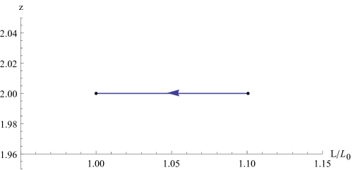
Figure 1: A solution with constant $z=2$ everywhere during the flow. The fixed point parameters are given by (47) along with $d=3$ and $\phi_{0}=1$. The arrow indicates the flow direction from UV to IR.

As far as we have investigated, no other solutions with $z\neq 2$ at the fixed points have constant $z(r)$ along the flow. This suggests that the additional Schrödinger symmetry for $z=2$ allows for consistent flows with constant $z$. In particular, imposing $z(r)=2$ and $H(r)=1$ reduces the system of equations (27) into four equations for two unknowns, $L(r)$ and $\phi(r)$. Since this system is over-constrained, some additional symmetry is needed for consistency. In this case, the key symmetry is the realization that $A^{\mu}\partial_{\mu}$ is a null Killing vector for this $z=2$ flow. The combination of the Maxwell and Killing equations then give the constraint

$$WA_{\nu}=\nabla^{\mu}F_{\mu\nu}=-2\nabla^{\mu}\nabla_{\nu}A_{\mu}=-2\nabla_{\nu}\nabla^{\mu}A_{\mu}-2R_{\nu}{}^{\lambda}A_{\lambda}.$$ (48)

Since the massive vector is divergence-free by its equation of motion, we are left with

$$R_{\mu\nu}A^{\nu}=-\frac{1}{2}W(\phi)A_{\mu}.$$ (49)

On the other hand, contraction of $A^{\lambda}$ with the Einstein equation

$$R_{\mu\nu}={\textstyle\frac{1}{2}}\partial_{\mu}\phi\partial_{\nu}\phi+{\textstyle\frac{1}{2}}(F_{\mu\lambda}F_{\nu}{}^{\lambda}-{\textstyle\frac{1}{2(d+1)}}g_{\mu\nu}F^{2})+{\textstyle\frac{2}{d+1}}g_{\mu\nu}V+{\textstyle\frac{1}{2}}A_{\mu}A_{\nu},$$ (50)

gives

$$R_{\mu\nu}A^{\nu}=\frac{2}{d+1}V(\phi)A_{\mu},$$ (51)

provided $A^{\mu}$ is a null Killing vector and $A^{\mu}\partial_{\mu}\phi=0$. Combining (49) with (51) then gives the condition

$$V(\phi)=-\frac{d+1}{4}W(\phi),$$ (52)

which indeed holds for $z_{IR}=z_{UV}=2$ in the cubic potential (43).

The relation (52) is a necessary condition for $A^{\mu}$ to be a null Killing vector. However, it only removes one redundancy in the equations of motion. The second redundancy comes from comparing the Maxwell equation in the first line of (27) with the combination of $ii$ and $tt$ Einstein equations in the third line of (27). Setting $H=1$ in these two equations gives

$$\begin{split}0&=z^{\prime}L-zL^{\prime}+z(z+d)-WL^{2},\\ 0&=2z^{\prime}L-zL^{\prime}+z(z+d)-WL^{2}+(z-2)(2z+d-L^{\prime}).\end{split}$$ (53)

These equations are redundant when $z(r)=2$, and we are left with a relatively simple system

$$\begin{split}0&=\phi^{\prime\prime}+\frac{d+2}{L}\phi^{\prime}-2\partial_{\phi}V,\\ 0&=L^{\prime}-(d+2)-\frac{2L^{2}}{d+1}V.\end{split}$$ (54)

for the two functions $\phi(r)$ and $L(r)$. ( Alternatively, the scalar equation can be replaced by the constraint (28).)

What we have shown is that, when the potential satisfies (52), the massive vector coupled to scalar model admits flows with $z=2$ and $H=1$ along the entire flow. Of course, we can also ask what happens when this constraint is not satisfied. As we now show, while it is still possible to flow from $z_{UV}=2$ to $z_{IR}=2$, the effective $z(r)$ will not be constant during the flow, and neither will $H(r)$.

3.3.2 Schrödinger flow with $z_{UV}=z_{IR}=2$, but changing $z$ in between

Since the potential relation (52) provides an additional symmetry allowing for constant $z=2$ flows, we may break this symmetry by adding another term to $V(\phi)$ in (43). In particular, we may add a quartic term to $V(\phi)$, while maintaining a cubic $W(\phi)$. One way to do this without affecting the UV and IR fixed point parameters is to add a term of the form

$$V(\phi)=V_{0}+V_{1}\phi+{\textstyle\frac{1}{2}}V_{2}\phi^{2}+{\textstyle\frac{1}{6}}V_{3}\phi^{3}+{\textstyle\frac{1}{24}}V_{4}\phi^{2}(\phi-\phi_{0})^{2},$$ (55)

where $V_{4}>0$, but is otherwise unconstrained. Since the flow is engineered to go from $\phi=0$ in the IR to $\phi=\phi_{0}$ in the UV, the additional term and its first derivative vanishes at the endpoints of the flow, thus ensuring that the fixed point data in (44) remains unchanged.

As an example of a flow with non-constant $z(r)$, we choose the same fixed point parameters (47) and take $V_{4}=24/\phi_{0}^{2}$. The numerical flow is shown in Fig. 2. Although $z(r)$ is no longer a constant along the flow, it starts and ends at the expected $z=2$ fixed points. This shows explicitly that, while $L(r)$ remains monotonic decreasing towards the IR (as it must by the null energy condition), $z(r)$ is certainly not monotonic.

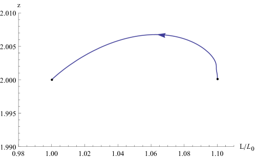
Figure 2: A solution with $z_{UV}=z_{IR}=2$ using the potential (55). The fixed point parameters are given by(47) along with $d=3$, $V_{4}=24/\phi_{0}^{2}$ and $\phi_{0}=1$. The arrow indicates the flow direction from UV to IR.

3.3.3 Schrödinger flow between different $z_{UV}$ and $z_{IR}$

The final example we consider is a flow with different fixed point $z$ values. We use the quartic $V(\phi)$ in (55) with $V_{4}=24/\phi_{0}^{2}$ along with the fixed point parameters

$$\begin{split}(L_{IR},\;z_{IR})&=(L_{0},\;21/10),\\ (L_{UV},\;z_{UV})&=(11L_{0}/10,\;2).\end{split}$$ (56)

The numerical solution is shown in Fig 3. This solution also exhibits monotonicity in $L$ toward the IR. However, it is worth noticing that this does not agree with the result in the appendix of Myers:2010tj , which claims that $L_{UV}>L_{IR}$ leads to $z_{UV}\geq z_{IR}$ in Schrödinger spacetimes.

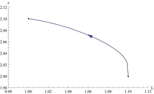
Figure 3: A solution flowing from $z_{UV}=2$ to $z_{IR}=2.1$. The fixed point parameters are given by (47) along with $d=3$, $V_{4}=24/\phi_{0}^{2}$ and $\phi_{0}=1$. The arrow indicates the flow direction from UV to IR.

4 Discussion

Our formulation of a Schrödinger $c$-theorem is given in terms of the effective radius $L(r)$. In the relativistic case, the AdS radius is directly related to the $a$ central charge according to (1). Hence monotonicity of $L(r)$ is equivalent to monotonicity of the corresponding $a(r)$ function. We would naturally like to make a similar connection between the effective radius and the scale anomaly in the non-relativistic case.

The non-relativistic version of the Weyl anomaly is the quantum breakdown of the Lifshitz scaling symmetry

$$t\to\lambda^{z}t,\qquad\vec{x}\to\lambda\vec{x}.$$ (57)

In particular, the anomaly is given by

$$z\langle T_{t}^{t}\rangle+\langle T_{i}^{i}\rangle=\mathcal{A},$$ (58)

where $\mathcal{A}$ can be constructed out of geometrical invariants. In contrast with the relativistic case, non-relativistic scaling provides fewer constraints on the form of $\mathcal{A}$ Adam:2009gq ; Gomes:2011di ; Griffin:2011xs ; Baggio:2011ha ; Arav:2014goa . Moreover, the invariants that contribute have dimension $d+z$ (where $d$ is the number of spatial dimensions) and may be formed out of a combination of time and space derivatives with dimensions $z$ and $1$, respectively. As a result, the structure of $\mathcal{A}$ depends very much on the values of $z$ and $d$.

In the case of $z=2$ and $d=2$ Lifshitz, $\mathcal{A}$ is dimension four and has two possible terms, with coefficients $C_{1}$ for a two time-derivative anomaly and $C_{2}$ for a four space-derivative anomaly Baggio:2011ha ; Arav:2014goa . A holographic calculation yields

$$C_{1}=\frac{1}{128\pi}\frac{2L}{G^{(4)}_{N}},\qquad C_{2}=0,$$ (59)

which demonstrates that the Lifshitz radius $L$ is indeed directly related to the scale anomaly. Similar results may be obtained for other values of $z$ and $d$.

We are, of course, more directly interested in the Schrödinger case, where there are additional Galilean symmetries. For $z=2$ Schrödinger, the Weyl anomaly was investigated in Jensen:2014hqa , and was shown to vanish for even-dimensional spacetimes (odd $d$). For odd-dimensional spacetimes, the lowest derivative anomaly has the same structure as the relativistic case in one dimension higher. It would be of interest to more directly connect this result with the radius $L$ that appears in Schrödinger holography.

Appendix A Modified weak energy condition for Lifshitz spacetime

In this appendix, we investigate the possibility of obtaining a holographic $c$-theorem from a modified weak energy condition in Lifshitz spacetime. We begin with the Lifshitz metric (7), which we repeat here for convenience

$$ds_{d+2}^{2}=-e^{2A(r)}dt^{2}+e^{2B(r)}d\vec{x}_{d}^{2}+dr^{2},$$ (60)

along with the definition (8) of the flow functions $L(r)$ and $z(r)$. The corresponding Einstein tensor is

$$\begin{split}G_{tt}&=\frac{g_{tt}}{L^{2}}d\left(-L^{\prime}+\frac{d+1}{2}\right),\\ G_{ij}&=\frac{g_{ij}}{L^{2}}\left(z^{\prime}L-(z+d-1)L^{\prime}+z^{2}+(d-1)z+\frac{d(d-1)}{2}\right),\\ G_{rr}&=\frac{d}{L^{2}}\left(z+\frac{d-1}{2}\right),\end{split}$$ (61)

and the Ricci scalar is

$$R=-\frac{2}{L^{2}}\left(z^{\prime}L-(z+d)L^{\prime}+z^{2}+dz+\frac{d(d+1)}{2}\right).$$ (62)

The consequences of the null energy condition on $L(r)$ and $z(r)$ were investigated in Liu:2012wf , and the resulting inequalities are

$$L^{\prime}\geq-(z-1),\qquad z^{\prime}\geq(z-1)(L^{\prime}-d-z)/L.$$ (63)

When $z\geq 1$, these inequalities may be combined to give (9). In any case, the null energy condition does not lead to monotonicity of $L(r)$. In an attempt to obtain a monotonic Lifshitz flow, we turn instead to the weak energy condition.

A.1 Weak energy condition

A conventional application of the weak energy condition is equivalent to the statement

$$G_{\mu\nu}t^{\mu}t^{\nu}\geq 0,$$ (64)

for all future-directed time-like vectors $t^{\mu}$. In this case, an upper bound for $L^{\prime}$ is achieved in the limit when $t^{\mu}$ approaches a null vector in the $t$–$x$ plane. The result coincides with the second inequality in (63), which may be expressed as

$$L^{\prime}\leq z+d+\frac{z^{\prime}L}{z-1}$$ (65)

(assuming $z>1$). On the other hand, a lower bound

$$L^{\prime}\geq\frac{d+1}{2},$$ (66)

achieved when $t^{\mu}$ is points purely at the time direction.

Note that this lower bound on $L^{\prime}$ is incompatible with having a Lifshitz fixed point (where $L$ would approach a constant). This is actually not surprising, as the presence of a negative cosmological constant, which can be expected in a Lifshitz background, can violate the weak energy condition. For a fixed cosmological constant, it is possible to modify the weak energy condition to exclude its contribution. Of course, it is not always possible to disentangle the contribution of a constant $\Lambda$ from a dynamical $\Lambda_{\rm eff}$. Nevertheless, we investigate this possibility.

A.2 Modified weak energy condition with an effective cosmological constant

Since the lower bound on $L^{\prime}$ given by (66) arises directly from the $G_{tt}$ in (61), we may remove the $(d+1)/2$ contribution by imposing a subtracted weak energy condition

$$(G_{\mu\nu}+\Lambda_{\rm eff}g_{\mu\nu})t^{\mu}t^{\nu}\geq 0.$$ (67)

Choosing

$$\Lambda_{\rm eff}=-\frac{d(d+1)}{2L^{2}}.$$ (68)

then gives

$$0\leq L^{\prime}\leq z+d+\frac{z^{\prime}L}{z-1}.$$ (69)

Note that $\Lambda_{\rm eff}$ is precisely the cosmological constant of pure AdS_d+2 with radius $L$.

Although this subtracted weak energy condition allows for both Lifshitz fixed points and monotonic flows for $L(r)$, it is not necessarily a well-defined energy condition on the matter fields. In particular, $\Lambda_{\rm eff}$ is implicitly defined through the flow function $L(r)$, which in turn is obtained from the metric function $A(r)$, and not directly from the matter sector. We thus turn away from this possibility and consider another modification to the weak energy condition that can be formulated more directly in terms of the stress tensor.

A.3 Modified weak energy condition with a Ricci scalar

Instead of an effective cosmological constant, we may add a geometric invariant to the left-hand side of (64). An obvious choice would be to use the Ricci scalar, so we consider a modification of the form

$$(G_{\mu\nu}+kg_{\mu\nu}R)t^{\mu}t^{\nu}\geq 0,$$ (70)

where $k$ is a constant that we adjust to achieve $L^{\prime}\geq 0$.

In Lifshitz spacetime with critical exponent $z$, choosing $k$ to be

$$k=\left(\frac{4z^{2}}{d(d+1)}+\frac{4z}{d+1}+2\right)^{-1},$$ (71)

then gives rise to the inequality

$$0\leq L^{\prime}\leq z+d,$$ (72)

where the lower bound is again achieved when $t$ points purely in the time direction, and the upper bound is achieved when $t$ approaches a null vector. Note that this result is the same as (69) when $z$ is constant.

In fact, for $k$ to be a constant, we must take $z$ to be a constant as well. Thus this modified weak energy condition is only applicable to Lifshitz flows where $z$ is held fixed. In this case, we can use the Einstein equation to rewrite (70) as a condition on the stress tensor

$$(T_{\mu\nu}-\frac{2k}{d-1}g_{\mu\nu}T)t^{\mu}t^{\nu}\geq 0.$$ (73)

In order to better understand the meaning of this energy condition, we consider a perfect fluid in Minkowski spacetime. In this case, (73) gives two conditions on the pressure $p$ and the density $\rho$

$$\rho+p\geq 0,\qquad\left(1-\frac{2k}{d}\right)\rho+\left(\frac{6k}{d}\right)p\geq 0.$$ (74)

This naturally limits to the usual weak energy condition

$$\rho+p\geq 0,\qquad\rho\geq 0,$$ (75)

in the limit $k\to 0$.

It is not entirely clear what the significance of such a modified weak energy condition is. Moreover, many Lifshitz flows of interest would not necessarily be constrained to have constant $z$. So, in the end, the possibility of obtaining a holographic $c$-theorem for Lifshitz spacetimes based on a physically well-motivated energy condition in the bulk remains an open question.

References

- (1) J. L. Cardy, Operator Content of Two-Dimensional Conformally Invariant Theories, Nucl. Phys. B 270 (1986) 186.
- (2) A. B. Zamolodchikov, Irreversibility of the Flux of the Renormalization Group in a 2D Field Theory, JETP Lett. 43 (1986) 730 [Pisma Zh. Eksp. Teor. Fiz. 43 (1986) 565].
- (3) L. Di Pietro and Z. Komargodski, Cardy Formulae for SUSY Theories in and , JHEP 1412 (2014) 031 [arXiv:1407.6061 [hep-th]].
- (4) A. A. Ardehali, J. T. Liu and P. Szepietowski, from the Superconformal Index, JHEP 1412 (2014) 145 [arXiv:1407.6024 [hep-th]].
- (5) Z. Komargodski and A. Schwimmer, On Renormalization Group Flows in Four Dimensions, JHEP 1112 (2011) 099 [arXiv:1107.3987 [hep-th]].
- (6) M. Henningson and K. Skenderis, The Holographic Weyl Anomaly, JHEP 9807 (1998) 023 [hep-th/9806087].
- (7) E. Álvarez and C. Gómez, Geometric Holography, the Renormalization Group and the -Theorem, Nucl. Phys. B 541 (1999) 441 [hep-th/9807226].
- (8) L. Girardello, M. Petrini, M. Porrati and A. Zaffaroni, Novel Local CFT and Exact Results on Perturbations of Super Yang Mills from AdS Dynamics, JHEP 9812 (1998) 022 [hep-th/9810126].
- (9) D. Z. Freedman, S. S. Gubser, K. Pilch and N. P. Warner, Renormalization Group Flows from Holography Supersymmetry and a -Theorem, Adv. Theor. Math. Phys. 3 (1999) 363 [hep-th/9904017].
- (10) V. Sahakian, Holography, a Covariant Function, and the Geometry of the Renormalization Group, Phys. Rev. D 62 (2000) 126011 [hep-th/9910099].
- (11) M. Taylor, Non-Relativistic Holography, arXiv:0812.0530 [hep-th].
- (12) Y. Nishida and D. T. Son, Nonrelativistic Conformal Field Theories, Phys. Rev. D 76 (2007) 086004 [arXiv:0706.3746 [hep-th]].
- (13) D. T. Son, Toward an AdS/Cold Atoms Correspondence: a Geometric Realization of the Schrödinger Symmetry, Phys. Rev. D 78 (2008) 046003 [arXiv:0804.3972 [hep-th]].
- (14) K. Balasubramanian and J. McGreevy, Gravity Duals for Non-Relativistic CFTs, Phys. Rev. Lett. 101 (2008) 061601 [arXiv:0804.4053 [hep-th]].
- (15) R. C. Myers and A. Sinha, Holographic -Theorems in Arbitrary Dimensions, JHEP 1101 (2011) 125 [arXiv:1011.5819 [hep-th]].
- (16) J. T. Liu and Z. Zhao, Holographic Lifshitz Flows and the Null Energy Condition, arXiv:1206.1047 [hep-th].
- (17) S. Moroz, Below the Breitenlöhner-Freedman Bound in the Nonrelativistic AdS/CFT Correspondence, Phys. Rev. D 81 (2010) 066002 [arXiv:0911.4060 [hep-th]].
- (18) T. Ishii and T. Nishioka, Flows to Schrödinger Geometries, Phys. Rev. D 84 (2011) 125007 [arXiv:1109.6318 [hep-th]].
- (19) H. Braviner, R. Gregory and S. F. Ross, Flows Involving Lifshitz Solutions, Class. Quant. Grav. 28 (2011) 225028 [arXiv:1108.3067 [hep-th]].
- (20) I. Adam, I. V. Melnikov and S. Theisen, A Non-Relativistic Weyl Anomaly, JHEP 0909 (2009) 130 [arXiv:0907.2156 [hep-th]].
- (21) P. R. S. Gomes and M. Gomes, On Ward Identities in Lifshitz-Like Field Theories, Phys. Rev. D 85 (2012) 065010 [arXiv:1112.3887 [hep-th]].
- (22) T. Griffin, P. Horava and C. M. Melby-Thompson, Conformal Lifshitz Gravity from Holography, JHEP 1205 (2012) 010 [arXiv:1112.5660 [hep-th]].
- (23) M. Baggio, J. de Boer and K. Holsheimer, Anomalous Breaking of Anisotropic Scaling Symmetry in the Quantum Lifshitz Model, JHEP 1207 (2012) 099 [arXiv:1112.6416 [hep-th]].
- (24) I. Arav, S. Chapman and Y. Oz, Lifshitz Scale Anomalies, JHEP 1502 (2015) 078 [arXiv:1410.5831 [hep-th]].
- (25) K. Jensen, Anomalies for Galilean Fields, arXiv:1412.7750 [hep-th].