Imperial-TP-AT-2015-07
Heat kernels on cone of $AdS_{2}$ and $k$-wound
circular Wilson loop in $AdS_{5}\times S^{5}$ superstring

We compute the one-loop correction to partition function of $AdS_{5}\times S^{5}$ superstring that should be representing $k$-fundamental circular Wilson loop in planar limit. The 2d metric of the minimal surface ending on $k$-wound circle at the boundary is that of a cone of $AdS_{2}$ with deficit $2\pi(1-k)$. We compute the determinants of 2d fluctuation operators by first constructing heat kernels of scalar and spinor Laplacians on the cone using Sommerfeld formula. The final expression for the $k$-dependent part of the one-loop correction has simple integral representation but is different from earlier results.

1 Introduction and summary

In this paper, which is a sequel to Appendix B in [1], we shall consider the computation of the disc partition function for the $AdS_{5}\times S^{5}\$superstring

$$Z=e^{-{\Gamma}}\ ,\ \ \ \ \ \qquad{\Gamma}={\Gamma}_{0}+{\Gamma}_{1}+...$$ (1.1)

for the euclidean minimal surface of ending on $k$-wound circle at the boundary. Here the expansion is in inverse powers of the string tension $T={{\sqrt{\lambda}}\ \over 2\pi}$ and we will be interested in first subleading (1-loop) correction ${\Gamma}_{1}$.

The string partition function should be representing [2, 3] the expectation value $\langle W\rangle$ of the circular Wilson loop in $k$-fundamental $SU(N)$ representation in dual ${\cal N}=4$ SYM theory taken in the limit $N\to\infty$ and then expanded in large ‘t Hooft coupling $\lambda$ for fixed $k$. The well-known exact expression for $\langle W\rangle$ in the planar approximation gives [4, 5, 6, 7]

$$\langle W\rangle={2\over k{\sqrt{\lambda}}\ }{I}_{1}(k{\sqrt{\lambda}}\ )=e^{-{\hat{\Gamma}}}\ ,\ \ \ \ \ \qquad{\hat{\Gamma}}={\hat{\Gamma}}_{0}+{\hat{\Gamma}}_{1}+...\ ,$$ (1.2)

$${\hat{\Gamma}}_{0}=-k{\sqrt{\lambda}}\ \ ,\qquad\qquad\textstyle{\hat{\Gamma}}_{1}={\textstyle{1\over 2}}\ln{\pi\over 2}+{3\over 2}\ln k+{3\over 2}\ln{\sqrt{\lambda}}\ \ .$$ (1.3)

Assuming that the planar $k$-fundamental circular Wilson loop is indeed represented by the open string path integral in $AdS_{5}\times S^{5}\$with the boundary condition that the disc-like world sheet ends on $k$-wound circle at the boundary the corresponding minimal surface in, e.g., $AdS_{3}$ with the metric $ds^{2}=z^{-2}(dr^{2}+r^{2}d\phi^{2}+dz^{2})$ is described by

$$\phi=k\tau\ ,\ \ \ \ \ z=\tanh k\sigma\ ,\ \ \ \ \ r=\cosh^{2}k\sigma\ ,\ \ \ \ \ \ \ z=\sqrt{1-r^{2}}\ ,$$ (1.4)

where $\tau\in(0,2\pi)\ ,\ \sigma\in(0,\infty)$. Then the induced metric is

$$ds^{2}={k^{2}\over\sinh^{2}k\sigma}(d\tau^{2}+d\sigma^{2})=d\xi^{2}+k^{2}\sinh^{2}\xi\,d\tau^{2}\ ,\qquad\qquad\textstyle\xi=\ln\tanh{k\sigma\over 2}\ .$$ (1.5)

For $k=1$ this is the usual $AdS_{2}$ metric but for $k=2,3,4,...,$ it has a conical singularity at $\xi=0$ with negative deficit $\delta=2\pi(1-k)$, i.e. this is a cone of $AdS_{2}$. The corresponding classical action is proportional to the regularized $AdS_{2}$ volume. To recall, the euclidean ${\widetilde{AdS}_{2}}$ space in Poincare coordinates $ds^{2}=z^{-2}(dx^{2}+dz^{2})$ with boundary being a line $R$ is not equivalent to $H_{2}=AdS_{2}$ in angular coordinates $ds^{2}=d\xi^{2}+\sinh^{2}\xi\,d\varphi^{2}$ with boundary $S^{1}$; in particular, their regularized volumes are different

$$V_{{\widetilde{AdS}_{2}}}={\ell\over\epsilon}\to\ 0\ ,\ \ \ \ \ \ \ \ \ \ \ \ \ V_{{{AdS}_{2}}}=2\pi({1\over\epsilon}-1)\to\ -2\pi\ .$$ (1.6)

Here we set the $AdS_{2}$ scale to 1, $\ell\to\infty$ is the length of the boundary of ${{\widetilde{AdS}_{2}}}$ and $\epsilon\to 0$ is a radial IR cutoff. As a result, the renormalized classical string action for (1.5) is ${\Gamma}_{0}=-k{\sqrt{\lambda}}\$ which matches the value of ${\hat{\Gamma}}_{0}$ in (1.3). This suggests that the prescription to use the regularized volume of $AdS_{2}$ is a required part of definition of string theory partition function in the context of AdS/CFT.

The starting point to compute ${\Gamma}_{1}$ is the general form of the $AdS_{5}\times S^{5}\$superstring one-loop correction [8, 9]

$${\Gamma}_{1}={\textstyle{1\over 2}}\ln\frac{[{\rm det}(-\nabla^{2}_{0})]^{5}\,[{\rm det}(-\nabla^{2}_{0}+2)]^{3}\ }{[{\rm det}(-\nabla^{2}_{{1\over 2}}+\frac{1}{4}R+1)]^{8}}\,.$$ (1.7)

In the simplest cases of minimal surfaces with symmetric-space induced metric (like $AdS_{2}$ spaces of straight line and circular loop) it is natural to preserve this symmetry in the loop computation till very end, i.e. not to introduce radial cutoff directly on contributions of individual modes [8, 1]. Then, as standard for determinants on a symmetric spaces [10, 11, 12] they can be computed using heat kernel technique (utilizing in an essential way the unbroken global symmetry) and the final expression will be proportional to the space volume factor for which we should use its renormalized value in (1.6). For example, in the straight line case the classical action and loop corrections will be proportional to the volume of $\widetilde{AdS}_{2}$ with boundary $R$ which has zero renormalized value in (1.6) and should thus be assumed to vanish [8, 13], in agreement with $\langle W\rangle=1$ on the gauge theory side.

Such heat kernel based computation of (1.7) in the $k=1$ circular loop case gives (using that the renormalized $V_{{{AdS}_{2}}}=-2\pi$) [8, 1]

$${\Gamma}_{1}(1)={\textstyle{1\over 2}}\ln(2\pi)\ .$$ (1.8)

The same expression was found in [13] using a different (Gelfand-Yaglom) method to compute the determinants with the radial IR cutoff implemented explicitly on modes and all power divergences dropped in the final expression. The same method applied to the $k>1$ case led to the following generalization of (1.8) [13]

$${\Gamma}_{1\,{\rm KT}}(k)={\textstyle{1\over 2}}\ln(2\pi)+(2k+{\textstyle{1\over 2}})\ln k-\ln k!\ .$$ (1.9)

This expression does not match the gauge theory result ${\hat{\Gamma}}_{1}$ in (1.3). The third $\ln{\sqrt{\lambda}}\$ term in ${\hat{\Gamma}}_{1}$ may be attributed to the presence of the string tension normalization factor for the three (Mobius-symmetry) ghost zero modes on the disc [5], which was not included in (1.7) and thus should be absent in (1.8),(1.9). The remaining difference may be coming from a numerical factor in normalization of the disc zero modes or from the ratio of the ghost and the two longitudinal mode determinants (assumed [8] to be equal to one in (1.7)) once they are computed with proper boundary conditions (cf. [14]).

Below we shall ignore these open issues and aim at just deriving the analog of (1.9) in the heat kernel approach of [8, 1]. Explicitly, we will find that

$${\Gamma}_{1}(k)={\textstyle{1\over 2}}k\ln(2\pi)+{\rm I}(k)\ ,\ \ \ \qquad\ \ \ \ \ {\rm I}(1)=0\ ,\qquad\qquad\ \$$ (1.10)

$${\rm I}(k)=-\frac{1}{4}\int_{0}^{\infty}{dy\over y\,\sinh y}\Big{[}(5e^{-y}+3e^{-3y})\big{(}\coth\frac{y}{k}-k\coth y\big{)}+16e^{-2y}\big{(}{1\over\sinh{y\over k}}-{k\over\sinh y}\big{)}\Big{]}$$ (1.11)

Here the terms with $e^{-y}$ and $e^{-3y}$ are the contributions of the scalar factors under log in (1.7) and the term with $e^{-2y}$ – the contribution of the spinor factor. For large $k$ the integral $I(k)$ is well approximated by a straight line, ${\rm I}(k)=c\,k+...,\ c=1.077$. This result for ${\Gamma}_{1}$ with $k>1$ is thus different from (1.9) of [13] and also different from the simple gauge-theory expression $\sim\ln k$ in (1.3).

Here we will not attempt to understand the difference with (1.9), concentrating on developing technical tools required for derivation of (1.11) that may have other potential applications. The main issue is to find scalar and fermion heat kernels on the cone of $AdS_{2}$ in (1.5). Let us mention also that another possible application of the above partition function is to computation of Rényi entropy on $AdS_{2}$ (see [15]).

It will be useful to replace $k$ in (1.5) by an arbitrary real number $\kappa$ and set $\kappa=k$ only at the end. Then if we take $\kappa$ to be equal to $1/n$ with an integer $n$ the metric (1.5) becomes that of an orbifold $AdS_{2}/Z_{n}$ (with a conical singularity of positive deficit) and the corresponding scalar or fermion heat kernel can be found as a sum over images [16, 17, 18]. This special case of $\kappa=1/n$ will thus allow us to check the general $\kappa$ expressions for heat kernels.

In the case of a cone of a 2-plane $ds^{2}=d\xi^{2}+\kappa^{2}\xi^{2}d\tau^{2}$ with a general $\kappa$ the scalar Laplacian heat kernel can be found using “re-periodisation” trick (or Sommerfeld formula) [19] and the same idea applies also to the construction of heat kernel on the cone of $AdS_{2}$ with generic $\kappa$ [16]. We shall present a detailed derivation of the expression of [16] for the scalar heat kernel in section 2.

The analogous construction for the spinor heat kernel can be given using the result [20, 21] for the regular $AdS_{2}$ and generalizing the examples of cones of 2-plane and 2-sphere in [22, 23]. We shall present it in section 3. This will be our main new technical result. As a check, we shall match the small $t$ expansion of the spinor kernel with the general form of asymptotic expansion of spinor heat kernel on a conical singularity in [24] and also show that in the special case of $\kappa=1/n$ corresponding to $AdS_{2}/Z_{n}$ orbifold it agrees with the result in [18].

In section 4 we shall use the results for the scalar and spinor heat kernels to compute the determinants in (1.7) deriving (1.11) and comparing it to (1.9).

In Appendix A we shall review the derivation of the Sommerfeld formula for heat kernels of 2d scalar and spinor Laplacians on a manifold with a conical singularity. In Appendix B we shall present the derivation of the phase factor matrix $U$ in the $AdS_{2}$ spinor heat kernel in (3.1).

2 Scalar heat kernel on cone of $AdS_{2}$

In order to compute the $1$-loop partition function (1.1),(1.7) we need to know the traces of heat kernels of the scalar and spinor Laplacians on the cone of $AdS_{2}$ with an arbitrary deficit $\delta=2\pi(1-\kappa)$ (we shall denote this space as $AdS_{2\kappa}$). In the regular $AdS_{2}$ case we have

$$\ln\det\Delta=-\int_{\epsilon}^{\infty}{dt\over t}\ {\rm K}(t)\ ,\ \ \ \ {\rm K}(t)=\int d^{2}x\sqrt{g}\ K(x,x;t)\ ,\ \ \ K(x,x^{\prime};t)=\big{\langle}x|e^{-t\Delta}|x^{\prime}\big{\rangle}\ \ \$$ (2.1)

$${\rm K}(t)=V_{{AdS_{2}}}K(t)\ ,\ \ \ \ \ \ \ \ \ \ \ K(t)=K(x,x;t)\ ,\ \ \ \ \ \ \ \ \ \ \ \ \ \ \ \ V_{{AdS_{2}}}=-2\pi\ .$$ (2.2)

Here ${\rm K}$ is the trace of heat kernel which on symmetric space is a product of (regularized) volume and heat kernel at coinciding points.

In this section we will review the computation of the heat kernel ${\rm K}$ of the scalar Laplacian $\Delta_{0}=-\nabla^{2}_{0}+m^{2}$ on $AdS_{2\kappa}$ using the Sommerfeld formula, rederiving the expression for it given in [16]. We shall check the consistency of the result in the special case when $\kappa=1/n$ with integer $n$ by comparing it with the scalar heat kernel on the orbifold $AdS_{2}/Z_{n}$.

The generalization of the scalar heat kernel on regular $AdS_{2}$ to the case of $AdS_{2\kappa}\$can be constructed using the Sommerfeld formula [19] as reviewed in Appendix A. The starting point is the expression for the untraced heat kernel of the scalar Laplacian on the regular $AdS_{2}$ [10, 11]

$$K_{AdS_{2}}(x,x^{\prime};t)=\frac{\sqrt{2}\,e^{-(m^{2}+{1\over 4})t}}{(4\pi t)^{{3}/{2}}}\int_{d(x,x^{\prime})}^{\infty}\frac{dy\ y\ e^{-\frac{y^{2}}{4t}}}{\sqrt{\cosh y-\cosh d(x,x^{\prime})}}\ .$$ (2.3)

Here $d(x,x^{\prime})$ is the geodesic distance between the two points $x=(\xi,\phi)$ and $x^{\prime}=(\xi^{\prime},\phi^{\prime})$ of $AdS_{2}$ in polar coordinates

$$ds^{2}=d\xi^{2}+\sinh^{2}\xi\,d\phi^{2}\ ,$$ (2.4)

$$\cosh d(x,x^{\prime})=\cosh\xi\,\cosh\xi^{\prime}-\sinh\xi\,\sinh\xi^{\prime}\,\cos(\phi-\phi^{\prime})\ .$$ (2.5)

According to the Sommerfeld formula, the traced heat kernel in presence of a conical singularity when $\phi\in(0,2\pi\kappa)$ is given by

$${\rm K}_{AdS_{2\kappa}}(t)\equiv{\rm K}_{\kappa}(t)=K(0;t)+\frac{i}{4\pi\kappa}\int_{\Gamma}dz\,\cot\frac{z}{2\kappa}\ K(z;t)\ ,$$ (2.6)

$$K(z;t)\equiv\int_{0}^{2\pi\kappa}d\phi\int_{0}^{\infty}d\xi\ \sinh\xi\ K(\xi=\xi^{\prime},\phi^{\prime}=\phi+z;t)\ ,$$ (2.7)

$$K(\xi=\xi^{\prime},\phi^{\prime}=\phi+z;t)=\frac{\sqrt{2}e^{-(m^{2}+{1\over 4})t}}{(4\pi t)^{3/2}}\int_{d(\xi,z)}^{\infty}\frac{dy\,y\,e^{-\frac{y^{2}}{4t}}}{\sqrt{\cosh y-\cosh d(\xi,z)}}\ ,$$ (2.8)

$$K(0;t)=\int_{0}^{2\pi\kappa}d\phi\int_{0}^{\infty}d\xi\ \sinh\xi\ K(\xi=\xi^{\prime},\phi^{\prime}=\phi;t)=\kappa\,{\rm K}_{AdS_{2}}(t)\ ,$$ (2.9)

$${\rm K}_{AdS_{2}}(t)=V_{{AdS_{2}}}\,K_{0}(t)\ ,\ \ \ \ \ \ \ K_{0}(t)=\frac{e^{-(m^{2}+{1\over 4})t}}{(4\pi t)^{{3}/{2}}}\int_{0}^{\infty}{dy\,y\,{1\over\sinh{y\over 2}}\,e^{-\frac{y^{2}}{4t}}}\ .\ \$$ (2.10)

Here $K(z;t)$ is the integrated heat kernel with points separated by $z$ along angular direction only. The contour $\Gamma$ on the complex plane is made of two vertical lines going from $-\pi+i\infty$ to $-\pi-i\infty$ and from $\pi-i\infty$ to $\pi+i\infty$ (see Appendix A). The geodesic distance $d(\xi,z)$ between the points $(\xi,\phi)$ and $(\xi,\phi+z)$ is given by $\sinh d(\xi,z)=|\sinh\xi\ \sin\frac{z}{2}|$.

In (2.10) we used that for regular symmetric $AdS_{2}$ space the heat kernel does not depend on coordinates at coinciding points. Note that the IR divergence regularized by $V_{{AdS_{2}}}\to-2\pi$ will be present only in the first “$AdS_{2}$” term $K(0;t)$ in (2.6), while the second integral term will be finite.

To compute $K(z;t)$ we introduce $v=\sinh\xi,\ \cosh d(v,z)=1+2v^{2}\sin^{2}\frac{z}{2}$ to get

$$K(z;t)=\frac{\kappa\ e^{-(m^{2}+{1\over 4})t}}{2(4\pi)^{{1}/{2}}\ t^{3/2}\ \sin{z\over 2}}\int_{0}^{\infty}\frac{dv\ v}{\sqrt{1+v^{2}}}\int_{d(v,z)}^{\infty}{dy\ y\ e^{-\frac{y^{2}}{4t}}\over\gamma^{2}(y,z)-v^{2}}\ ,\,\ \qquad\gamma(y,z)\equiv\frac{\sinh{\frac{y}{2}}}{\sin{\frac{z}{2}}}\ .$$ (2.11)

Now we interchange the integration limits $\int_{0}^{\infty}dv\int_{d(v,z)}^{\infty}dy=\int_{0}^{\infty}dy\int_{0}^{d^{-1}(y,z)}dv,\ \$ and integrate over $v$ using $\int_{0}^{\gamma(y,z)}\frac{dv\ v}{\sqrt{1+v^{2}}\sqrt{\gamma^{2}(y,z)-v^{2}}}=\frac{\pi}{2}-\arctan\gamma^{-1}(y,z)$. Then integrating by parts one finds that

$$K(z;t)=\frac{\kappa}{(4\pi t)^{{1}/{2}}\sin{z\over 2}}\int_{0}^{\infty}dy\ e^{-{y^{2}\over 4t}}\ \frac{\cosh{y\over 2}\ \sin{z\over 2}}{\cosh y-\cos z}\ .$$ (2.12)

Changing the variable $y\rightarrow 2y$ we finally get

$$K(z;t)=\frac{\kappa\ e^{-(m^{2}+{1\over 4})t}}{(4\pi t)^{{1}/{2}}}\int_{0}^{\infty}dy\ e^{-{y^{2}\over t}}\ \frac{\cosh y}{\sinh^{2}y+\sin^{2}{z\over 2}}\ .$$ (2.13)

According to (2.6), the scalar heat kernel on cone of $AdS_{2}$ is thus given by

$${\rm K}_{\kappa}(t)=\kappa\,{\rm K}_{AdS_{2}}(t)+\frac{\kappa\ e^{-(m^{2}+{1\over 4})t}}{(4\pi t)^{{1}/{2}}}\int_{0}^{\infty}dy\ \cosh y\ e^{-{y^{2}\over t}}\ \frac{i}{4\pi\kappa}\int_{\Gamma}dz\ F(z;y,\kappa)\ ,$$ (2.14)

$$F(z;y,\kappa)=\frac{1}{\sinh^{2}y+\sin^{2}{z\over 2}}\ \cot\frac{z}{2\kappa}\ .$$ (2.15)

For $\kappa=1$ the function $F(z,y;\kappa)$ becomes $2\pi$ periodic in $z$, and due to the structure of the contour $\Gamma$, this leads to the vanishing of the integral contribution.

To evaluate the contour integral we use the residue theorem. The two vertical lines $(-\pi+i\infty,-\pi-i\infty)$ and $(\pi-i\infty,\pi+i\infty)$ surround one pole of $\cot\frac{z}{2\kappa}$ at $z=0$ with the residue $\mathrm{Res}\ F(z=0;y,\kappa)=\frac{2\kappa}{\sinh^{2}y}$. Setting $y=-iu$ we get $F(z;u,\kappa)=\frac{\cot\frac{z}{2\kappa}}{(\sin\frac{z}{2}+\sin u)(\sin\frac{z}{2}-\sin u)}$ with two poles on the imaginary axis at $z=\pm 2u$. Using the limit

$$\lim_{z\rightarrow\pm 2u}\frac{\sin\frac{z}{2}\pm\sin u}{z\pm 2u}={\textstyle{1\over 2}}\cos u$$ (2.16)

we find

$$\mathrm{Res}\ F(z=\pm 2u;u,\kappa)=\frac{\cot\frac{u}{\kappa}}{\sin u\cos u}=-\frac{\coth\frac{y}{\kappa}}{\sinh y\cosh y}.$$ (2.17)

Therefore

$$\frac{i}{4\pi\kappa}\int_{\Gamma}dz\,F(z;y,\kappa)=2\pi i\ \frac{i}{4\pi\kappa}\Big{(}\frac{2\kappa}{\sinh^{2}y}-\frac{2\coth\frac{y}{\kappa}}{\sinh y\ \cosh y}\Big{)}=\frac{1}{\sinh^{2}y}\Big{(}\frac{\tanh y}{\kappa\tanh\frac{y}{\kappa}}-1\Big{)}\ .$$ (2.18)

Finally, the scalar heat kernel on $AdS_{2\kappa}$ is given by

$${\rm K}_{\kappa}(t)=\kappa\,{\rm K}_{AdS_{2}}(t)+\frac{e^{-(m^{2}+{1\over 4})t}}{(4\pi t)^{{1}/{2}}}\int_{0}^{\infty}dy\ e^{-\frac{y^{2}}{t}}\frac{1}{\sinh y}\big{(}\coth\frac{y}{\kappa}-\kappa\,\coth y\big{)}\ ,$$ (2.19)

which is the same expression as given in [16].

The integral vanishes for $\kappa=1$, i.e. ${\rm K}_{\kappa=1}(t)={\rm K}_{AdS_{2}}(t)$. It is obviously convergent at $y\to\infty$ and also at $y\rightarrow 0$ since $\frac{\coth\frac{y}{\kappa}-\kappa\coth y}{\sinh y}\big{|}_{y\to 0}\to\frac{1}{3}({\kappa}^{-1}-\kappa)+O(y)$.

The special case of $\kappa=1/n$ corresponds to the $Z_{n}$ orbifold of $AdS_{2}$ which is obtained by identification $\phi=\phi+\frac{2\pi}{n}$. The analog of the Sommerfeld formula for orbifolds is equivalent to the summation over images expression discussed in [18]. There it was found that the small $t$ expansion of the heat kernel for a massless scalar Laplacian on $AdS_{2}/Z_{n}$ is given by

$${\rm K}_{AdS_{2}/Z_{n}}(t)=\textstyle\frac{1}{n}{\rm K}_{AdS_{2}}(t)+\frac{n^{2}-1}{12n}-\frac{(n^{2}+11)(n^{2}-1)}{360n}\,t+O(t^{2})\ .$$ (2.20)

To compare to the general expression (2.19) we need first to set there $m=0$ and expand for small $t$. Changing the variable $y\rightarrow\sqrt{t}\,u$ we get for $t\to 0$

$$\begin{split}{\rm K}_{\kappa}(t)=&\kappa\,{\rm K}_{AdS_{2}}(t)+\frac{\kappa(1-\frac{t}{4})}{(4\pi)^{{1/2}}}\int_{0}^{\infty}du\ e^{-u^{2}}\ \textstyle\big{[}\frac{1}{3}\big{(}\frac{1}{\kappa^{2}}-1\big{)}+\frac{7\kappa^{4}-5\kappa^{2}-2}{90\kappa^{4}}\,t\,u^{2}\big{]}+O(t^{2})\\ =&\kappa\,{\rm K}_{AdS_{2}}(t)+\textstyle\frac{1}{12}\big{(}\kappa^{-1}-\kappa\big{)}-\frac{1+10\kappa^{2}-11\kappa^{4}}{360\kappa^{3}}\,t+O(t^{2})\ .\end{split}$$ (2.21)

Setting here $\kappa=1/n$ we indeed match the orbifold expansion (2.20).

3 Spinor heat kernel on cone of $AdS_{2}$

Let us now turn to the spinor case. The fermions in (1.7) are real (Majorana) so that log of their determinant or trace of heat kernel should be understood with extra ${\textstyle{1\over 2}}$ included (so that on a trivial background the contribution of one 2d Majorana fermion is minus that of one real scalar). The starting point is the heat kernel for the (Majorana) spinor Laplacian $\Delta_{1\over 2}=-\nabla^{2}_{1\over 2}+{1\over 4}R+m^{2}$ on $AdS_{2}$ [20]

$$K(x,x^{\prime};t)=U(x,x^{\prime})\,\frac{e^{-m^{2}t}}{\sqrt{2}\,(4\pi t)^{3/2}}{1\over\cosh{d(x,x^{\prime})\over 2}}\int_{d(x,x^{\prime})}^{\infty}\frac{dy\,y\,\cosh\frac{y}{2}\,e^{-\frac{y^{2}}{4t}}}{\sqrt{\cosh y-\cosh d(x,x^{\prime})}}\ .$$ (3.1)

Here $U(x,x^{\prime})$ is a $2\times 2$ matrix acting on the $AdS_{2}$ spinor bundle and satisfying the equation of the parallel transport along the geodesic connecting the two points $(x,x^{\prime})$:

$$n^{\mu}(x,x^{\prime})\nabla_{\mu}U(x,x^{\prime})=0\ ,\qquad U(x,x)=I\ ,\qquad n_{\mu}(x,x^{\prime})=\nabla_{\mu}\,d(x,x^{\prime})=\partial_{\mu}\,d(x,x^{\prime})\ .$$ (3.2)

Here the derivatives are taken with respect to the point $x$ and $n_{\mu}(x,x^{\prime})$ is the tangent vector to the geodesic. The general structure of $U(x,x^{\prime})$ on hyperbolic spaces was not spelled out in the literature. As we show in Appendix B in the present case of $AdS_{2}$ in polar coordinates (2.4) it is given by ($\sigma_{3}$ is the Pauli matrix)

$$U(\xi,\xi^{\prime},\phi,\phi^{\prime})=\exp\Big{(}i\sigma_{3}\,\arctan\frac{\cosh\frac{\xi+\xi^{\prime}}{2}\,\tan\frac{\phi-\phi^{\prime}}{2}}{\cosh\frac{\xi-\xi^{\prime}}{2}}\Big{)}\ .$$ (3.3)

We can now apply the fermionic version of the Sommerfeld formula (see Appendix A) to obtain the heat kernel of the spinor Laplacian on the cone of $AdS_{2}$ (cf. (2.6),(2.7))

$${\rm K}_{\kappa}(t)=\mathrm{Tr\,}K(0;t)+\frac{i}{4\pi\kappa}\int_{\Gamma}dz\ \frac{1}{\sin\frac{z}{2\kappa}}\ \mathrm{Tr\,}K(z;t)\ ,$$ (3.4)

$$\mathrm{Tr\,}K(z;t)\equiv\int_{0}^{2\pi\kappa}d\phi\int_{0}^{\infty}d\xi\,\sinh\xi\ \mathrm{Tr\,}K(\xi=\xi^{\prime},\phi^{\prime}=\phi+z;t)\ ,$$ (3.5)

$$\mathrm{Tr\,}K(\xi=\xi^{\prime},\phi^{\prime}=\phi+z;t)=\mathrm{Tr\,}U(\xi,z)\,\frac{e^{-m^{2}t}}{\sqrt{2}\,(4\pi t)^{3/2}}{1\over\cosh{d(\xi,z)\over 2}}\int_{d(\xi,z)}^{\infty}\frac{dy\,y\,\cosh\frac{y}{2}\,e^{-\frac{y^{2}}{4t}}}{\sqrt{\cosh y-\cosh d(\xi,z)}}$$

$$U(\xi,z)=\exp\Big{[}i\sigma_{3}\arctan\big{(}\cosh\xi\tan\frac{z}{2}\big{)}\big{]}\ ,\qquad\ \mathrm{Tr\,}U(\xi,z)=\frac{2}{\sqrt{1+\cosh^{2}\xi\ \tan^{2}{z\over 2}}}\ ,$$ (3.6)

$$\mathrm{Tr\,}K(0;t)=\mathrm{Tr\,}K(x,x;t)=\kappa\,{\rm K}_{AdS_{2}}(t)\ ,\ \ \qquad{\rm K}_{AdS_{2}}(t)=V_{AdS_{2}}K_{{}_{1\over 2}}(t)\ ,$$ (3.7)

$$K_{{}_{1\over 2}}(t)=\frac{e^{-m^{2}t}}{(4\pi t)^{3/2}}\int_{0}^{\infty}{dy\,y\,\coth\frac{y}{2}\,e^{-\frac{y^{2}}{4t}}}\ .$$ (3.8)

Here $K(x,x^{\prime};t)=K(\xi,\xi^{\prime},\phi,\phi^{\prime};t)$ is the fermionic kernel in the regular $AdS_{2}$ case in (3.1). The contour $\Gamma$ is the same as in the scalar case in (2.6) (see Appendix A).

To compute $\mathrm{Tr\,}K(z;t)$ in (3.5) we integrate over the angle and after a change of variables ($v=\sinh\xi,\ \ \cosh d=1+2v^{2}\sin^{2}\frac{z}{2}$) we find

$$\mathrm{Tr\,}K(z;t)=\frac{\kappa\,e^{-m^{2}t}}{(4\pi)^{{1}/{2}}\,t^{3/2}}\int_{0}^{\infty}\frac{dv\,v}{\sqrt{1+v^{2}}}\frac{\cos{z\over 2}}{1+v^{2}\sin^{2}{z\over 2}}\int_{d(v,z)}^{\infty}\frac{dy\,y\,\cosh\frac{y}{2}\,e^{-\frac{y^{2}}{4t}}}{\sqrt{\sinh^{2}\frac{y}{2}-v^{2}\sin^{2}\frac{z}{2}}}.$$ (3.9)

Interchanging the integration limits as explained below (2.11) we get

$$\begin{split}&\mathrm{Tr}\,K(z;t)=\frac{\kappa\,e^{-m^{2}t}}{(4\pi)^{{1}/{2}}\,t^{3/2}\sin{z\over 2}}\int_{0}^{\infty}dy\,y\,\cosh\frac{y}{2}\,e^{-{y^{2}\over 4t}}\ G(y,z),\\ &G(y,z)\equiv\int_{0}^{\gamma(y,z)}{dv\over\sqrt{1+v^{2}}}\,\frac{v\ \cos{z\over 2}}{\sqrt{\gamma^{2}(y,z)-v^{2}}\ (1+v^{2}\sin^{2}{z\over 2})}\ ,\end{split}$$ (3.10)

where $\gamma(y,z)={\sinh\frac{y}{2}\over\sin\frac{z}{2}}$ as in (2.11). As a result

$$G(y,z)=\frac{1}{\cosh{y\over 2}}\big{(}{\pi\over 2}-\arctan\frac{\tan{z\over 2}}{\tanh{y\over 2}}\big{)}\ .$$ (3.11)

Integrating by parts in the remaining integral over $y$ in (LABEL:355) one can put it into the form

$$\mathrm{Tr}\,K(z;t)=\frac{\kappa\,e^{-m^{2}t}}{(4\pi t)^{{1/2}}\sin{z\over 2}}\int_{0}^{\infty}dy\ e^{-{y^{2}\over 4t}}\ \frac{\sin z}{\cosh y-\cos z}\ .$$ (3.12)

Changing the variable $y\rightarrow 2y$ gives

$$\mathrm{Tr}\,K(z;t)=\frac{2\kappa\,e^{-m^{2}t}}{(4\pi t)^{{1/2}}}\int_{0}^{\infty}dy\ e^{-{y^{2}\over t}}\ \frac{\cos{z\over 2}}{\sinh^{2}y+\sin^{2}{z\over 2}}\ ,$$ (3.13)

so that (3.4) takes the form (cf. (2.14))

$${\rm K}_{\kappa}(t)=\kappa\,{\rm K}_{AdS_{2}}(t)+\frac{2\kappa\,e^{-m^{2}t}}{(4\pi t)^{{1/2}}}\int_{0}^{\infty}dy\,e^{-{y^{2}\over t}}\ \frac{i}{4\pi\kappa}\int_{\Gamma}dz\ F_{{}_{1\over 2}}(z;y,\kappa)\ ,$$ (3.14)

$$F_{{}_{1\over 2}}(z;y,\kappa)=\ \frac{1}{\sinh^{2}y+\sin^{2}{z\over 2}}\ \frac{\cos\frac{z}{2}}{\sin{z\over 2\kappa}}\ .$$ (3.15)

For $\kappa=1$ the function $F_{{}_{1\over 2}}(z,y;\kappa)$ becomes the same as $F(z,y;\kappa)$ in (2.15) in the scalar case, so that the second integral term vanishes because of the structure of the contour $\Gamma$.

It remains to evaluate the contour integral using the residue theorem. As in the scalar case, the contour $\Gamma$ contains one pole of $\frac{1}{\sin{z\over 2\kappa}}$ at $z=0$ and two imaginary poles $z=\pm 2iy$ of $\frac{1}{\sinh^{2}y+\sin^{2}{z\over 2}}$, i.e. (cf. (2.18))

$$\frac{i}{4\pi\kappa}\int_{\Gamma}dz\ F_{{}_{1\over 2}}(z;y,\kappa)=-\frac{1}{\sinh y}\big{(}\frac{1}{\kappa\sinh\frac{y}{\kappa}}-\frac{1}{\sinh y}\big{)}\ .$$ (3.16)

Finally, the spinor heat kernel the $AdS_{2\kappa}$ is given by

$${\rm K}_{\kappa}(t)=\kappa\,{\rm K}_{AdS_{2}}(t){-}\frac{2\,e^{-m^{2}t}}{(4\pi t)^{{1/2}}}\int_{0}^{\infty}dy\ e^{-\frac{y^{2}}{t}}\ \frac{1}{\sinh y}\,\big{(}\frac{1}{\sinh\frac{y}{\kappa}}-\frac{\kappa}{\sinh y}\big{)}\ .$$ (3.17)

The integral term here vanishes at $\kappa=1$ and is convergent at both $y\to\infty$ and $y\to 0$ where $\frac{1}{\sinh y}\big{(}\frac{1}{\kappa\sinh\frac{y}{\kappa}}-\frac{1}{\sinh y}\big{)}\to\frac{1}{y}\big{[}\big{(}\frac{1}{y}-\frac{y}{6\kappa^{2}}\big{)}-\big{(}\frac{1}{y}-\frac{y}{6}\big{)}\big{]}=\frac{1}{6}\big{(}1-\frac{1}{\kappa^{2}}\big{)}.$

To check (3.17) we may compare its small $t$ expansion with the asymptotic expansion of spinor heat kernel in the case of a general curved manifold with a conical singularity derived in [24]. Setting $m=0$ in (3.17) and changing $y\rightarrow\sqrt{t}\,u$ we get

$${\rm K}_{\kappa}(t)=\kappa\,{\rm K}_{AdS_{2}}(t){-}\frac{2\kappa}{(4\pi)^{{1/2}}}\int_{0}^{\infty}du\ e^{-u^{2}}\ \frac{1}{\sinh(\sqrt{t}\,u)}\ \big{[}\frac{1}{\kappa\sinh(\frac{\sqrt{t}\,u}{\kappa})}-\frac{1}{\sinh(\sqrt{t}\,u)}\big{]}\ ,$$ (3.18)

so that expanding in small $t$ gives

$${\rm K}_{\kappa}(t)=\kappa\,{\rm K}_{AdS_{2}}(t)\textstyle+\frac{1}{12}({\kappa^{-1}}-\kappa)+\frac{17\kappa^{4}-10\kappa^{2}-7}{1440\kappa^{3}}\,t+O(t^{2})\ ,$$ (3.19)

in agreement with general expressions in [24]. As in the scalar case, we may also match (3.19) with the small $t$ expansion of the the massless spinor heat kernel on $AdS_{2}/Z_{n}$ in [18] corresponding to the special case of $\kappa={1\over n}$ (cf. (2.20))

$${\rm K}_{AdS_{2}/Z_{n}}(t)=\textstyle\frac{1}{n}{\rm K}_{AdS_{2}}(t)+\frac{n^{2}-1}{12n}-\frac{(7n^{2}+17)(n^{2}-1)}{1440n}\,t+O(t^{2})\ .$$ (3.20)

4 One-loop partition function

Let us now apply the above results for heat kernels (2.19) and (3.17) to compute the $AdS_{5}\times S^{5}\$string partition function (1.1),(1.7) on the cone $AdS_{2\kappa}$. Using the explicit values of masses ($m^{2}_{0}=0,2$ and $m^{2}_{1\over 2}=1$) in (1.7) and (2.1) we get

$${\Gamma}_{1}(\kappa)=\kappa\,{\Gamma}_{1}(1)+{\rm I}(\kappa)\ ,\qquad\ \ \ \ \ \ \ \ {\Gamma}_{1}(1)={\textstyle{1\over 2}}\ln(2\pi)\ ,\$$ (4.1)

$${\rm I}(\kappa)=-{\textstyle{1\over 2}}\int^{\infty}_{\varepsilon}{dt\over t}\int_{0}^{\infty}{dy}\ {e^{-\frac{y^{2}}{t}}\over(4\pi t)^{{1}/{2}}}\ H(t,y;\kappa)\ ,$$ (4.2)

$$H(t,y;\kappa)={1\over\sinh y}\Big{[}(5e^{-{1\over 4}t}+3e^{-{9\over 4}t})\big{(}\coth\frac{y}{\kappa}-\kappa\,\coth y\big{)}+16e^{-{t}}\big{(}\frac{1}{\sinh\frac{y}{\kappa}}-\frac{\kappa}{\sinh y}\big{)}\Big{]}\ .\ \ \ \$$ (4.3)

Here we isolated the contribution $\kappa\,{\Gamma}_{1}(1)$ of the first ($AdS_{2}$) terms in (2.19) and (3.17) where ${\Gamma}_{1}(1)$ given by (1.8) was already computed in [1]. The first term in the bracket in $H$ is the combined contribution of 5+3 scalars and the second term is the contribution of 8 fermions (taken with the minus sign as required in (1.7)). Both vanish for $\kappa=1$, i.e. $H(t,y;1)=0$.

The proper time integral is actually convergent at $t\to 0$ as one can see from the small $t$ expansion of the heat kernels in (2.21) and (3.19) or directly from (4.2),(4.3) after setting $y\to y=\sqrt{t}\,u$ to get $\int_{0}^{\infty}{dy}\ {e^{-\frac{y^{2}}{t}}\over(4\pi t)^{{1}/{2}}}\to\int_{0}^{\infty}{du}\ {e^{-u^{2}}\over(4\pi)^{{1}/{2}}}$:

$$H(t,\sqrt{t}\,u;\kappa)\Big{|}_{t\to 0}=-{\textstyle{2\over 15}}(\kappa-\kappa^{-3})u^{2}\,t+O(t^{2})\ .$$ (4.4)

The resulting cancellation of 2d UV divergences in (4.2) is an important check of the consistency of this result as the (non-trivial part of the) 1-loop correction in $AdS_{5}\times S^{5}\$superstring should be finite on generic 2d background [8].

We can thus remove the proper-time (UV) cutoff $\varepsilon$ in (4.2) and compute the finite integral over $t$ (keeping $t$ and $y$ as integration variables and using that $\int_{0}^{\infty}\frac{dt}{t^{3/2}}e^{-(\mu^{2}t+\frac{y^{2}}{t})}=\frac{\sqrt{\pi}}{y}e^{-2\mu y}$)

$${\rm I}(\kappa)=-\frac{1}{4}\int_{0}^{\infty}{dy\over y\,\sinh y}\Big{[}(5e^{-y}+3e^{-3y})\big{(}\coth\frac{y}{\kappa}-\kappa\coth y\big{)}+16e^{-2y}\big{(}{1\over\sinh{y\over\kappa}}-{\kappa\over\sinh y}\big{)}\Big{]}\ .$$ (4.5)

This integral is convergent at both $y\to\infty$ and $y\to 0$ as for small $y$ the integrand goes as ${1\over 6}(\kappa-\kappa^{-1})+O(y)$.

It is not clear how to compute the integral (4.5) analytically. For some integer values of $\kappa$ it is given by a combination of values of the Riemann $\zeta$-function and polygamma functions, but we could not find an interpolating expression. It is of course straightforward to evaluate it numerically and conclude that for $\kappa=k\not=1$ it is different from the earlier result (1.9) of [13] and also from the gauge-theory ${3\over 2}\ln k$ behaviour in (1.3). We illustrate the difference between ${\Gamma}_{1}(k)$ in (4.1) and ${\Gamma}_{1,\rm KT}(k)$ in (1.9) in Figure 1. For large $\kappa$ we find that ${\Gamma}_{1}$ grows linearly, ${\Gamma}_{1}(\kappa\gg 1)\to 1.077\kappa$, while for small $\kappa$ we get ${\Gamma}_{1}(\kappa\to 0)\to-0.15\kappa^{-1}$.

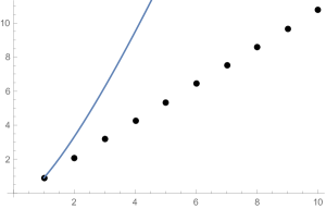
Figure 1: Comparison between ${\Gamma}_{1}(k)$ in (4.1) (black dots) and ${\Gamma}_{1\,\rm KT}(k)$ in (1.9) (blue line)

Appendix A Heat kernels of Laplacians on 2d cone

Let us consider a $2$-dimensional space with a radial coordinate $\xi$ and a polar angle $\phi$ of period $\beta=2\pi\kappa$ with metric near $\xi=0$ being $ds^{2}=d\xi^{2}+\xi^{2}d\phi^{2}$ so that there is a conical singularity with angular deficit $\delta=2\pi-\beta=2\pi(1-\kappa)$. Given the expression for the heat kernel of a scalar or spinor Laplacian on a regular manifold ($\kappa=1$) it is possible to derive its counterpart on the space with $\kappa\not=1$ using so called Sommerfeld formula [19, 24]. We shall review this construction below.

A.1 Scalar case

Let us consider first the case of flat 2d cone

$$ds^{2}=d\xi^{2}+\xi^{2}d\phi^{2}\ ,\ \ \ \ \ \ \ \ \ \ \ \phi+2\pi\kappa\equiv\phi\ .$$ (A.1)

To construct the heat kernel for $\Delta=-\partial^{\mu}\partial_{\mu}$ on this cone it is sufficient to consider the two points $x(\phi)=(\xi,\phi)$ and $x(0)=(\xi,0)$ separated only in the angular direction by angle $\phi$. The starting point is the heat kernel for $\kappa=1$, i.e. on a regular $R^{2}$ plane, where we have for $K(x,x^{\prime};t)=\big{\langle}x|e^{-t\Delta}|x^{\prime}\big{\rangle}$

$$K(x(\phi),x(0);t)\equiv K_{0}(\xi,\phi,\ \xi,0;t)=\frac{1}{4\pi t}\,e^{-{1\over 4t}{|x(\phi)-x(0)|^{2}}}=\frac{1}{4\pi t}\,e^{-{1\over 2t}(1-\cos\phi){\xi^{2}}}\ .$$ (A.2)

Since this is a smooth function of $\phi$, we can rewrite it using the Cauchy representation:

$$K(x(\phi),x(0);t)=\frac{1}{2\pi i}\oint_{C}\frac{dz}{z-\phi}K(x(z),x(0);t)\ ,$$ (A.3)

where $C$ is a contour in the complex plane which encircles the point $z=\phi$. Now let us deform $C$ to a family of contours $A_{n},\ n=0,\pm 1,\pm 2,....$, where $A_{n}$ goes from $(2n+1)\pi-\epsilon+i\infty$ to $(2n-1)\pi+\epsilon+i\infty$ in the higher half plane and from $(2n-1)\pi+\epsilon-i\infty$ to $(2n+1)\pi-\epsilon-i\infty$ in the lower half plane one. Then the heat kernel can be expressed as the “sum over images”

$$K(x(\phi),x(0);t)=\frac{1}{2\pi i}\sum_{n=-\infty}^{\infty}\int_{A_{n}}\frac{dz}{z-\phi}K(x(z),x(0);t)\qquad\qquad$$

$$=\frac{1}{2\pi i}\sum_{n=-\infty}^{\infty}\int_{A_{0}}\frac{dz}{z-\phi-2\pi n}K(x(z),x(0);t)=\frac{1}{4\pi i}\int_{A_{0}}dz\,\cot\frac{z-\phi}{2}\ K(x(z),x(0);t)\ .$$ (A.4)

Here we used the periodicity of the kernel in (A.2) and the identity $\sum_{n=-\infty}^{\infty}\frac{1}{z-nq}=\frac{\pi}{q}\cot\frac{\pi z}{q}\ .$

We can now repeat the same procedure changing the period of the angle from $2\pi$ to $2\pi\kappa$ to get the heat kernel on the cone (A.1)

$$K_{\kappa}(x(\phi),x(0);t)=\frac{1}{4\pi i\kappa}\int_{A_{0}}dz\,\cot\frac{z-\phi}{2\kappa}\ K(x(\phi),x(0);t)\ ,$$ (A.5)

or after shifting $z\rightarrow z+\phi$

$$K_{\kappa}(x(\phi),x(0);t)=\frac{1}{4\pi i\kappa}\int_{A_{0}^{\prime}}dz\,\cot\frac{z}{2\kappa}\,K(x(z+\phi),x(0);t)\ .$$ (A.6)

The contour $A_{0}^{\prime}$ is obtained from $A_{0}$ by a shift by $\phi$ and consists of two pieces: one in the upper half plane running from $\pi+\phi+i\infty$ to $-\pi+\phi+i\infty$ and one in the lower half plane going from $-\pi+\phi-i\infty$ to $\pi+\phi-i\infty$. We may then deform $A_{0}^{\prime}$ into a small circle around $z=0$ and another contour $\Gamma^{\prime}$ made of two vertical lines: one going from $-\pi+\phi-i\infty$ to $-\pi+\phi+i\infty$ and one from $\pi+\phi+i\infty$ to $\pi+\phi-i\infty$. Near $z=0$ the integrand has a pole of $\cot\frac{z}{2\kappa}\sim\frac{2\kappa}{z}$ with residue being the regular plane kernel $K(x(z+\phi),x(0);t)$. Then denoting $\Gamma=-\mathrm{\Gamma^{\prime}}$ we finish with

$$K_{\kappa}(x(\phi),x(0);t)=K(x(\phi),x(0);t)+\frac{i}{4\pi\kappa}\int_{\Gamma}dz\,\cot\frac{z}{2\kappa}\ K(x(z+\phi),x(0);t)\ .$$ (A.7)

This is the Sommerfeld formula for the heat kernel of the scalar Laplacian on the cone (A.1) in terms of the heat kernel on the regular 2-plane.

The same procedure can be applied to the case of an arbitrary space $\mathcal{M}$ where the heat kernel depends only on the angular distance between two points. Denoting $x=(\xi,\phi)$, $x^{\prime}=(\xi^{\prime},\phi^{\prime})$ the coordinates of two points on the corresponding cone $\mathcal{M}_{\kappa}$ of $\mathcal{M}$, the Sommerfeld formula for the heat kernel of the scalar Laplacian reads

$$K_{\kappa}(\xi,\xi^{\prime},\phi,\phi^{\prime};t)=K(\xi,\xi^{\prime},\phi,\phi^{\prime};t)+\frac{i}{4\pi\kappa}\int_{\Gamma}dz\,\cot\frac{z}{2\kappa}\ K(\xi,\xi^{\prime},\phi+z,\phi^{\prime};t).$$ (A.8)

Here the angular distance is $z=\phi-\phi^{\prime}$ and the contour $\Gamma$ is formed by two vertical lines from $-\pi+(\phi-\phi^{\prime})+i\infty$ to $-\pi+(\phi-\phi^{\prime})-i\infty$ and from $\pi+(\phi-\phi^{\prime})-i\infty$ to $\pi+(\phi-\phi^{\prime})+i\infty$. Taking the coincident points limit we get

$$K_{\kappa}(\xi=\xi^{\prime},\phi=\phi^{\prime};t)=K(\xi=\xi^{\prime},\phi=\phi^{\prime};t)+\frac{i}{4\pi\kappa}\int_{\Gamma}dz\,\cot\frac{z}{2\kappa}\ K(\xi=\xi^{\prime},\phi^{\prime}=\phi+z;t)\ .$$ (A.9)

Defining the integrated heat kernel

$$K(z;t)=\int_{M_{\kappa}}d\phi\,d\xi\,\sqrt{g}\ K(\xi=\xi^{\prime},\phi^{\prime}=\phi+z;t)\ ,$$ (A.10)

we finally get the expression for the trace of heat kernel

$${\rm K}_{\kappa}(t)=\int_{M_{\kappa}}d^{2}x\,\sqrt{g}\,\big{\langle}x|e^{-t\Delta}|x\big{\rangle}=K(0;t)+\frac{i}{4\pi\kappa}\int_{\Gamma}dz\,\cot\frac{z}{2\kappa}\ K(z;t)\ .$$ (A.11)

Since in (A.11) $\phi=\phi^{\prime}$, here the contour $\Gamma$ reduces to two vertical lines going from $-\pi-i\infty$ to $-\pi+i\infty$ and from $\pi-i\infty$ to $\pi+i\infty$.

Thus in addition to the expected term $K(0;t)$ “inherited” from the regular space case there is a correction given by a contour integral on the complex plane. For $\kappa=1$ this second term vanishes as expected: the integrand becomes $2\pi$ periodic in $z$ and the contributions coming from the integration along the two vertical lines at $-\pi$ and $\pi$ cancel each other.

A.2 Spinor case

Let us start again with a flat space cone. On $R^{2}$ in Cartesian coordinates the spin connection is trivial and the fermionic Laplace operator $\Delta_{{1\over 2}}=-{\nabla}^{2}+\frac{1}{4}{R}$ reduces to the scalar Laplacian $\Delta_{0}=-\partial^{\mu}\partial_{\mu}$. Thus solution to the heat kernel equation is the same as for the scalar (A.2) up to $2\times 2$ identity matrix $I$:

$$\tilde{K}\left(x,x^{\prime};t\right)=K_{0}(x,x^{\prime};t)\,I\ .$$ (A.12)

In polar coordinates $(\xi,\phi)$ the spinor covariant derivative is $\nabla_{\mu}=\partial_{\mu}+\omega_{\mu}$ with $\omega_{\mu}dx^{\mu}=-\frac{i}{2}\sigma_{3}d\phi$. Thus

$$\nabla_{\mu}={\rm V}\partial_{\mu}V^{-1}\ ,\ \ \ \ \ \ \ \ \ \Delta_{1\over 2}={\rm V}\Delta_{0}{\rm V}^{-1}\ ,\qquad\qquad{\rm V}=e^{\frac{i}{2}\sigma_{3}\phi}\ .$$ (A.13)

Then the solution to the spinor heat kernel equation in polar coordinates may be written as

$$K(x,x^{\prime};t)={\rm V}(\phi)\,\tilde{K}(x,x^{\prime};t)\ ,$$ (A.14)

with $\tilde{K}$ given by (A.12). Due to the presence of the spin factor ${\rm V}$ the spinor heat kernel is antiperiodic in $\phi$.

To get spinor heat kernel on a cone of $R^{2}$ we follow the same route as in the scalar case: we choose $x(\phi)=(\xi,\phi)$, $x(0)=(\xi,0)$ and first rewrite $K(x,x^{\prime};t)$ in (A.14) using the method of the images as in (A.3),(A.4):

$$K(x(\phi),x(0);t)=\frac{1}{2\pi i}\oint_{C}{\frac{dz}{z-\phi}\,{\rm V}(z)\,K(x(z),x(0);t)}$$

$$\qquad\qquad\qquad\quad=\frac{1}{2\pi i}\sum_{n=-\infty}^{\infty}\int_{A_{n}}\frac{dz}{z-\phi}\ {\rm V}(z)\,K(x(z),x(0);t)$$

$$\qquad\qquad\qquad\quad=\frac{1}{2\pi i}\sum_{n=-\infty}^{\infty}\int_{A_{0}}\frac{dz\,(-1)^{n}}{z-\phi-2\pi n}\,{\rm V}(z)\,K(x(z),x(0);t)$$

$$\qquad\qquad\qquad\quad=\frac{1}{4\pi i}\int_{A_{0}}\,dz\,\frac{1}{\sin\frac{z-\phi}{2}}\,{\rm V}(z)\,K(x(z),x(0);t)\ .$$ (A.15)

Here we used the antiperiodicity of ${\rm V}$ and $\sum_{n=-\infty}^{\infty}\frac{(-1)^{n}}{z-qn}=\frac{\pi}{q}\frac{1}{\sin\frac{\pi z}{q}}$. We can now change the periodicity of $\phi$ from $2\pi$ to $2\pi\kappa$ and to get the expression for the spinor heat kernel on the cone of $R^{2}$

$$K_{\kappa}(x(\phi),x(0);t) = \frac{1}{4\pi i\kappa}\int_{A_{0}}\,dz\ \frac{1}{\sin\frac{z-\phi}{2\kappa}}\,K(x(z),x(0);t)$$ (A.16)

$$= \frac{1}{4\pi i\kappa}\int_{A_{0}^{\prime}}\,dz\ \frac{1}{\sin\frac{z}{2\kappa}}\,K(x(z+\phi),x(0);t)\ ,$$

where $A_{0}^{\prime}$ is again given by two lines in the upper and lower half plane: one running from $\pi+\phi+i\infty$ to $-\pi+\phi+i\infty$ and the other from $-\pi+\phi-i\infty$ to $\pi+\phi-i\infty$. Next, we deform $A_{0}^{\prime}$ into a small circle around $z=0$ and a contour $\Gamma^{\prime}$ made of two vertical lines that run from $-\pi+\phi-i\infty$ to $-\pi+\phi+i\infty$ and from $\pi+\phi+i\infty$ to $\pi+\phi-i\infty$. Setting $\Gamma=-\Gamma^{\prime}$ we obtain

$$K_{\kappa}(x(\phi),x(0);t)=K(x(\phi),x(0);t)+\frac{i}{4\pi\kappa}\int_{\Gamma}\,dz\ \frac{1}{\sin\frac{z}{2\kappa}}\,K(x(z+\phi),x(0);t)\ .$$ (A.17)

This expression can be generalized to the case of a cone of curved 2d space where the heat kernel depends on the angular distance between two points $x=(\xi,\phi)$ and $x^{\prime}=(\xi^{\prime},\phi^{\prime})$

$$K_{\kappa}(\xi,\xi^{\prime},\phi,\phi^{\prime};t)=K(\xi,\xi^{\prime},\phi,\phi^{\prime};t)+\frac{i}{4\pi\kappa}\int_{\Gamma}\,dz\frac{1}{\sin\frac{z}{2\kappa}}\,K(\xi,\xi^{\prime},\phi+z,\phi^{\prime};t)\ .$$ (A.18)

Here, as in the scalar case in (A.8), $\Gamma$ is modified by $\phi\rightarrow\phi-\phi^{\prime}$. Defining the integrated kernel as in (A.10) we then get the final expression for the traced spinor heat kernel:

$${\rm K}_{\kappa}(t)=\mathrm{Tr}\,K(0;t)+\frac{i}{4\pi\kappa}\int_{\Gamma}\,dz\ \frac{1}{\sin\frac{z}{2\kappa}}\,\mathrm{Tr}\,K(z;t)\ .$$ (A.19)

Here $\mathrm{Tr\,}$ is over the spinor indices and the integration contour reduces for $\phi=\phi^{\prime}$ to the two vertical lines going from $-\pi-i\infty$ to $-\pi+i\infty$ and from $\pi-i\infty$ to $\pi+i\infty$. For $\kappa=1$ the integrand becomes periodic (as the product of two antiperiodic functions in $z$) and thus the integral contribution vanishes.

Appendix B Matrix $U$ in spinor heat kernel on $AdS_{2}$

Here we solve the equation (3.2) for the matrix $U$ in the $AdS_{2}$ metric (2.4) written in polar coordinates. The corresponding zweibein and tangent space and spinor connections are ($\mu=(\xi,\phi)$)

$$e^{1}_{\mu}=(1,0)\ ,\ \ \ \ \ e^{2}_{\mu}=(0,\sinh\xi)\ ,\ \ \ \ \ \ \ \ \omega_{\xi}^{\alpha\beta}=0\ ,\ \ \ \ \ \ \omega_{\phi}^{12}=-\omega_{\phi}^{21}=-\cosh\xi\ ,$$ (B.1)

$$\omega_{\mu}={1\over 2}\omega_{\mu}^{\alpha\beta}\Sigma_{\alpha\beta}=(0,-\frac{i}{2}\cosh\xi\ \sigma_{3})\ ,\ \ \ \ \ \ \ \ \Sigma_{\alpha\beta}={1\over 4}[\gamma_{\alpha},\gamma_{\beta}]\ ,\ \ \ \ \ \ \gamma^{\alpha}=(\sigma_{1},\sigma_{2})\ .$$ (B.2)

In [20] it was shown that (3.2) is equivalent to the requirement that the spinor covariant derivative acts on $U(\xi,\xi^{\prime},\phi,\phi^{\prime})$ in the following way

$$\textstyle\nabla_{\mu}U=\partial_{\mu}U+\omega_{\mu}\,U=A\,\Sigma_{\alpha\beta}\,n^{\beta}\,U\ ,\ \ \ \ \ \ \ \ A\equiv\tanh\frac{d(\xi,\xi^{\prime},\phi,\phi^{\prime})}{2}\ ,$$ (B.3)

where the geodesic distance between the two points $(\xi,\phi)\ ,(\xi^{\prime},\phi^{\prime})$ is given in (2.5). This equation for $U$ can be rewritten as

$$\partial_{\xi}U=\frac{i}{2}{\tanh{d\over 2}\over{\sinh\xi}\,}{\partial_{\phi}d}\,\sigma_{3}U\ ,\qquad{\partial_{\phi}U}=\frac{i}{2}{\sinh\xi}\big{(}\coth\xi-\tanh\frac{d}{2}\,\partial_{\xi}d\big{)}\,\sigma_{3}U\ .$$ (B.4)

The first equation in (B.4) has solution

$$U(\xi,\xi^{\prime},\phi,\phi^{\prime})=\exp\big{[}\frac{i}{2}\sigma_{3}B(\xi,\xi^{\prime},\phi,\phi^{\prime})\big{]}\,C(\phi,\phi^{\prime})\ ,$$ (B.5)

$$B(\xi,\xi^{\prime},\phi,\phi^{\prime})=\int{d\xi\over\sinh\xi}\ \partial_{\phi}\log\big{[}1+\cosh d(\xi,\xi^{\prime},\phi,\phi^{\prime})\big{]}\ .$$ (B.6)

Using (2.5) we find

$$B = \int{d\xi\over\sinh\xi}\ \frac{\sinh\xi\sinh\xi^{\prime}\sin(\phi-\phi^{\prime})}{1+\cosh\xi\cosh\xi^{\prime}-\sinh\xi\sinh\xi^{\prime}\cos(\phi-\phi^{\prime})}$$ (B.7)

$$= 2\arctan\frac{\cosh\frac{\xi+\xi^{\prime}}{2}\ \tan\frac{\phi-\phi^{\prime}}{2}}{\cosh\frac{\xi-\xi^{\prime}}{2}}-{\pi}\ .$$

The matrix $C(\phi,\phi^{\prime})$ can be determined from the second equation in (B.4)

$$\partial_{\phi}C=\frac{i}{2}\sigma_{3}\big{(}\cosh\xi-\sinh\xi\tanh\frac{d}{2}\,\partial_{\xi}d-\partial_{\phi}B\big{)}C=0\ ,$$ (B.8)

where we used (2.5) and (B.7). Thus $C$ is constant and is fixed by the initial condition $U(\xi=\xi^{\prime},\phi=\phi^{\prime})=I$

$$C(\phi,\phi^{\prime})=e^{\frac{i}{2}\pi\sigma_{3}}=i\sigma_{3}\ .$$ (B.9)

As a result,

$$U(\xi,\xi^{\prime},\phi,\phi^{\prime})=\exp\Big{(}i\sigma_{3}\,\arctan\frac{\cosh\frac{\xi+\xi^{\prime}}{2}\,\tan\frac{\phi-\phi^{\prime}}{2}}{\cosh\frac{\xi-\xi^{\prime}}{2}}\Big{)}\ .$$ (B.10)

References

• [1] E. I. Buchbinder and A. A. Tseytlin, “1/N correction in the D3-brane description of a circular Wilson loop at strong coupling,” Phys. Rev. D 89, no. 12, 126008 (2014) [arXiv:1404.4952].
• [2] D. E. Berenstein, R. Corrado, W. Fischler and J. M. Maldacena, “The Operator product expansion for Wilson loops and surfaces in the large N limit,” Phys. Rev. D 59, 105023 (1999) [hep-th/9809188].
• [3] N. Drukker, D. J. Gross and H. Ooguri, “Wilson loops and minimal surfaces,” Phys. Rev. D 60, 125006 (1999) [hep-th/9904191].
• [4] J. K. Erickson, G. W. Semenoff and K. Zarembo, “Wilson loops in N=4 supersymmetric Yang-Mills theory,” Nucl. Phys. B 582, 155 (2000) [hep-th/0003055]. G. W. Semenoff and K. Zarembo, “Wilson loops in SYM theory: From weak to strong coupling,” Nucl. Phys. Proc. Suppl.  108, 106 (2002) [hep-th/0202156].
• [5] N. Drukker and D. J. Gross, “An Exact prediction of N=4 SUSYM theory for string theory,” J. Math. Phys.  42 (2001) 2896 [hep-th/0010274].
• [6] N. Drukker and B. Fiol, “All-genus calculation of Wilson loops using D-branes,” JHEP 0502 (2005) 010 [hep-th/0501109].
• [7] V. Pestun, “Localization of gauge theory on a four-sphere and supersymmetric Wilson loops,” Commun. Math. Phys.  313, 71 (2012) [arXiv:0712.2824].
• [8] N. Drukker, D.J. Gross and A.A. Tseytlin, “Green-Schwarz string in AdS(5) x S5: Semiclassical partition function,” JHEP 0004 (2000) 021 [hep-th/0001204].
• [9] S. Forste, D. Ghoshal and S. Theisen, “Stringy corrections to the Wilson loop in N=4 superYang-Mills theory,” JHEP 9908, 013 (1999) [hep-th/9903042].
• [10] I. Chavel, “Heat kernels and spectral theory”, Cambridge U.P., 1984.
• [11] R. Camporesi, “Harmonic analysis and propagators on homogeneous spaces,” Phys. Rept.  196 (1990) 1.
• [12] D. Fursaev and D. Vassilevich, “Operators, Geometry and Quanta : Methods of spectral geometry in quantum field theory,” D. V. Vassilevich, “Heat kernel expansion: User’s manual,” Phys. Rept.  388, 279 (2003) [hep-th/0306138].
• [13] M. Kruczenski and A. Tirziu, “Matching the circular Wilson loop with dual open string solution at 1-loop in strong coupling,” JHEP 0805 (2008) 064 [arXiv:0803.0315].
• [14] C. Kristjansen and Y. Makeenko, “More about One-Loop Effective Action of Open Superstring in $AdS_{5}\times S^{5}$,” JHEP 1209 (2012) 053 [arXiv:1206.5660].
• [15] S. N. Solodukhin, “Entanglement entropy, conformal invariance and extrinsic geometry,” Phys. Lett. B 665, 305 (2008) [arXiv:0802.3117]. H. Casini and M. Huerta, “Entanglement entropy for the n-sphere,” Phys. Lett. B 694, 167 (2010) [arXiv:1007.1813 [hep-th]]. I. R. Klebanov, S. S. Pufu, S. Sachdev and B. R. Safdi, “Renyi Entropies for Free Field Theories,” JHEP 1204, 074 (2012) [arXiv:1111.6290]. R. Aros, F. Bugini and D. E. Diaz, “On Renyi entropy for free conformal fields: holographic and q-analog recipes,” J. Phys. A 48, 105401 (2015) [arXiv:1408.1931].
• [16] R. B. Mann and S. N. Solodukhin, “Universality of quantum entropy for extreme black holes,” Nucl. Phys. B 523, 293 (1998) [hep-th/9709064].
• [17] T.H. Jones and D. Kucerovsky, “Heat Kernel for Simply-Connected Riemann Surfaces”, arXiv:1007.5467 [math.DG].
T.H. Jones, “The heat kernel on noncompact Riemann surfaces”, PhD thesis (2008).
• [18] R. K. Gupta, S. Lal and S. Thakur, “Heat Kernels on the $AdS_{2}$ cone and Logarithmic Corrections to Extremal Black Hole Entropy,” JHEP 1403 (2014) 043 [arXiv:1311.6286]. “Logarithmic Corrections to Extremal Black Hole Entropy in N = 2, 4 and 8 Supergravity,” arXiv:1402.2441.
• [19] J. S. Dowker, “Quantum Field Theory on a Cone,” J. Phys. A 10, 115 (1977). “Vacuum Averages for Arbitrary Spin Around a Cosmic String,” Phys. Rev. D 36, 3742 (1987). D. V. Fursaev, “The Heat kernel expansion on a cone and quantum fields near cosmic strings,” Class. Quant. Grav.  11, 1431 (1994) [hep-th/9309050]. J. S. Dowker, “Effective actions with fixed points,” Phys. Rev. D 50, 6369 (1994) [hep-th/9406144].
• [20] R. Camporesi, “The Spinor heat kernel in maximally symmetric spaces,” Commun. Math. Phys.  148 (1992) 283. R. Camporesi and A. Higuchi, “Spectral functions and zeta functions in hyperbolic spaces,” J. Math. Phys.  35 (1994) 4217.
• [21] R. Camporesi and A. Higuchi, “On the Eigen functions of the Dirac operator on spheres and real hyperbolic spaces,” J. Geom. Phys.  20, 1 (1996) [gr-qc/9505009].
• [22] D. N. Kabat, “Black hole entropy and entropy of entanglement,” Nucl. Phys. B 453, 281 (1995) [hep-th/9503016].
• [23] D. V. Fursaev and G. Miele, “Cones, spins and heat kernels,” Nucl. Phys. B 484, 697 (1997) [hep-th/9605153].
• [24] D. V. Fursaev, “Euclidean and canonical formulations of statistical mechanics in the presence of killing horizons,” Nucl. Phys. B 524, 447 (1998) [hep-th/9709213].