Amplitude and frequency variations of oscillation modes
in the pulsating DB white dwarf star KIC 08626021

Abstract

Context. The signatures of nonlinear effects affecting stellar oscillations are difficult to observe from ground observatories due to the lack of continuous high precision photometric data spanning extended enough time baselines. The unprecedented photometric quality and coverage provided by the Kepler spacecraft offers new opportunities to search for these phenomena.

Aims. We use the Kepler data accumulated on the pulsating DB white dwarf KIC 08626021 to explore in detail the stability of its oscillation modes, searching in particular for evidences of nonlinear behaviors.

Methods. We analyse nearly two years of uninterrupted short cadence data, concentrating on identified triplets caused by stellar rotation that show intriguing behaviors during the course of the observations.

Results. We find clear signatures of nonlinear effects that could be attributed to resonant mode coupling mechanisms. These couplings occur between the components of the triplets and can induce different types of behaviors. We first notice that a structure at 3681 $\mu$Hz identified as a triplet in previous published studies is in fact forming a doublet with the third component being an independent mode. We find that a triplet at 4310 $\mu$Hz and this doublet at 3681 $\mu$Hz (most likely the two visible components of an incomplete triplet) have clear periodic frequency and amplitude modulations typical of the so-called intermediate regime of the resonance, with time scales consistent with theoretical expectations. Another triplet at 5073 $\mu$Hz is likely in a narrow transitory regime in which the amplitudes are modulated while the frequencies are locked. Using nonadiabatic pulsation calculations based on a model representative of KIC 08626021 to evaluate the linear growth rates of the modes in the triplets, we also provide quantitative information that could be useful for future comparisons with numerical solutions of the amplitude equations.

Conclusions. The observed modulations are the clearest hints of nonlinear resonant couplings occurring in white dwarf stars identified so far. These should resonate as a warning to projects aiming at measuring the evolutionary cooling rate of KIC 08626021, and of white dwarf stars in general. Nonlinear modulations of the frequencies can potentially jeopardize any attempt to measure reliably such rates, unless they can be corrected beforehand. These results should motivate further theoretical work to develop the nonlinear stellar pulsation theory.

1 Introduction

The temporal variations of the amplitude and frequency of oscillation modes often seen, or suspected, in pulsating stars cannot be explained by the linear nonradial stellar oscillation theory (Unno et al., 1989) and must be interpreted in the framework of a nonlinear theory. It is believed that nonlinear mechanisms such as resonant mode couplings could generate such modulations, as, e.g., in the helium dominated atmosphere (DB) white dwarf star GD 358 (Goupil et al., 1998). Resonant couplings are for instance predicted to occur when slow stellar rotation produces triplet structures whose component frequencies satisfy the relation $\nu_{+}+\nu_{-}\sim 2\nu_{0}$, where $\nu_{0}$ is the frequency of the central $m=0$ mode. The theoretical exploration of these mechanisms was extensively developed in Buchler et al. (1995, 1997), but was almost interrupted more than a decade ago because of the lack of clear observational evidence of such phenomena, due to the difficulty of capturing amplitude or frequency variations that occur on months to years timescales from ground based observatories. Nevertheless, the presence of resonant couplings within rotationally split mode triplets was proposed for the first time as the explanation for the frequency and amplitude long term variations observed in the GW Vir pulsator PG 0122+200 (Vauclair et al., 2011) from successive campaigns on this object. This suggests that pulsating white dwarfs could be among the best candidates to detect and test the nonlinear resonant coupling theory.

White dwarfs constitute the ultimate evolutionary fate expected for $\sim 98\%$ of the stars in our Galaxy. While cooling down, they cross several instability strips in which they develop observable nonradial $g$-mode oscillations. Among these, the helium atmosphere DB white dwarfs representing $\sim 20\%$ of all white dwarfs, are found to pulsate in the effective temperature range of 21,000 K to 28,000 K (Beauchamp et al., 1999; Fontaine & Brassard, 2008; Winget & Kepler, 2008). All classes of pulsating white dwarfs are particularly valuable for probing their interior with asteroseismology, but it has also been proposed that hot DB pulsators with apparently stable modes could be used to measure their cooling rate, which is dominated by neutrino emission (Winget et al., 2004). The secular rates of change for the pulsation periods in hot DB pulsators is expected to be $\sim 10^{-13}$ ss^-1, corresponding to a time scale of 3$\times 10^{5}$ years. However, this possibility could be seriously impaired by other phenomena affecting the pulsation frequencies on shorter timescales. Such variations in amplitude and frequency have indeed been suspected in several white dwarf stars (e.g. PG 0122+200, Vauclair et al., 2011; WD 0111+0018, Hermes et al., 2013; HS 0507+0434B, Fu et al., 2013), as stellar evolution theory cannot explain the variations with estimated timescales at least two orders of magnitude shorter than the expected cooling rates. Nonlinear effects on stellar pulsations, including resonant mode coupling mechanisms could induce such modulations and need to be considered carefully (Vauclair, 2013).

In this context, observations from space of a multitude of pulsating stars including white dwarfs has open up new horizons. The Kepler spacecraft monitored a 105 deg² field in the Cygnus-Lyrae region for nearly four years without interruption, obtaining unprecedented high quality photometric data for asteroseismology (Gilliland et al., 2010). These uninterrupted data are particularly suited to search for long term temporal frequency and amplitude modulations of the oscillation modes.

Among the 6 pulsating white dwarfs discovered in the Kepler field, KIC 08626021 (a.k.a., WD J1929+4447 or GALEX J192904.6+444708) is the only identified DB pulsator (Østensen et al., 2011). Based on the first month of short cadence (SC) Kepler data, Østensen et al. (2011) estimated that this star has an average rotation period $P_{\rm rot}\sim 1.7$ days, derived from the observed frequency spacings of 3 groups of $g$-modes interpreted as triplets due to rotation. Subsequent independent efforts to isolate a seismic model for KIC 08626021 from Bischoff-Kim & Østensen (2011) and Córsico et al. (2012) both suggest that the effective temperature of the star is significantly hotter than the value determined from the survey spectroscopy. However, the masses determined from these two models are not consistent with each other. More recently, a new asteroseismic analysis based on the full Kepler data set provided by Bischoff-Kim et al. (2014) confirmed the former results found by Bischoff-Kim & Østensen (2011).We point out that a new asteroseismic analysis of KIC 08626021 is discussed in Giammichele et al. (2015).

KIC 08626021 has been observed by Kepler for nearly two years in SC mode without interruption since the quarter Q10. Thus, it is a suitable candidate to investigate the long term amplitude and frequency modulations of the oscillation modes occurring in this star. In this paper we present a new thorough analysis of the Kepler lightcurve obtained on the DB pulsator KIC 08626021, emphasizing in particular the time dependence of the amplitudes and frequencies of the modes associated to rotationally split triplets (Section 2). We provide arguments linking the uncovered amplitude and frequency modulations to the nonlinear mode coupling mechanisms (Section 3), before summarizing and concluding (Section 4).

2 The frequency content of KIC 08626021 revisited

The pulsating white dwarf star KIC 08626021 has been continuously observed by Kepler in short cadence (SC) mode from quarter Q10.1 to Q17.2 (when the second inertial wheel of the satellite failed). A lightcurve from Q7.2, well disconnected from the main campaign, is also available for that star. Some analyses of these data have already been reported in the literature (Østensen et al., 2011; Córsico et al., 2012), including most recently the asteroseismic study of Bischoff-Kim et al. (2014, hereafter BK14) based on the full Q10.1 – Q17.2 data set. We initially considered using these published results as the starting point of our present study, but we realized that important details were lacking for our specific purposes. Consequently, we detail below, as a necessary step, our own thorough analysis of the frequency content of KIC 08626021.

2.1 The Kepler photometry

All the data gathered by Kepler for that star are now in the public domain. We obtained the lightcurves from the Mikulski Archive for Space Telescopes (MAST). As is standard, these data were processed through the Kepler Science Processing Pipeline (Jenkins et al, 2010). In the following, we concentrate on the consecutive data covering Q10.1 to Q17.2 without considering Q7.2 that would introduce a large time gap in the assembled lightcurve. With this restriction, we are left with a mere 23 months of high precision photometric data starting from BJD 2 455 740 and ending on BJD 2 456 424 ($\sim$ 684 days) with a duty cycle of $\sim 87\%$.

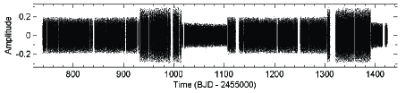
Figure 1: Top panel: Condensed representation of the full Kepler lightcurve (Amplitude is the residual relative to the mean brightness intensity of the star vs time in Barycentric Julian Date) covering from Q10.1 to Q17.2 ($\sim 684$ days) of KIC 08626021. Between quarters, scatter sometime changes due to different levels of noise in the data (all quarters are not equivalent in photometric quality). Bottom panel: Close-up view showing one day of the Kepler lightcurve by slices of 0.1 days. At this scale the oscillations are clearly apparent.

We constructed the full lightcurve from each quarter ”corrected” lightcurves, which most notably include a correction for the amplitude due to the contamination of the star by a closeby object (this correction consider that only $\sim 47.3\%$ of the light comes from the DB white dwarf). Tests indicate that the main differences between these corrected data and the raw data set used by BK14 occur in the measured amplitudes of the light variations, but has otherwise no noticeable incidence on the extracted frequencies. Each quarter light curve was then individually corrected to remove residual long term trends (using sixth-order polynomial fits) and data points differing significantly from the local standard deviation of the lightcurve were removed by applying a running 3-$\sigma$ clipping filter. The later operation just very slightly decreases the overall noise level.

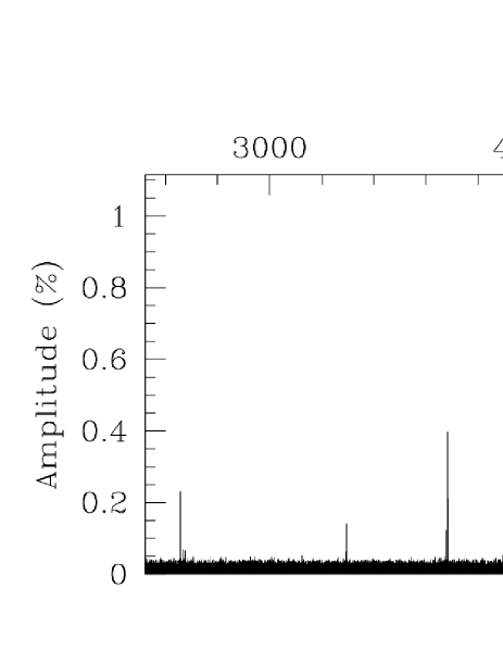
Figure 2: Lomb-Scargle Periodogram (LSP; Amplitude in % of the mean brightness vs frequency in $\mu$Hz) of the Kepler lightcurve. The represented range covers the frequency region where the pulsation modes are detected (no significant signal is found outside these limits). Note that some well known Kepler instrumental artefacts are within this frequency range but can easily be recognized.

The resulting ligthcurve is shown in Figure 1 and the corresponding Lomb-Scargle Periodogram (LSP; Scargle 1982) is given in Figure 2. The low-amplitude multi-periodic modulations are clearly seen with dominant periodicities of the order of a few minutes, typical of $g$-mode oscillations observed in pulsating DB white dwarfs. The formal frequency resolution in the Lomb-Scargle periodogram (defined as the inverse of the total time base line of the observations) reaches $\sim 0.017$ $\mu$Hz.

2.2 Defining a secure detection threshold

Before proceeding with the extraction of the frequencies, a brief discussion of the criteria used to define the confidence level of the detections is necessary. With ground based observations of pulsating compact stars, a widely used rule of thumb was to consider the limit of $4\sigma$ (4 times the average local noise in the Fourier Transform) as the threshold above which a signal could safely be considered as real. However, with space observations, in particular with Kepler, it became increasingly clear that this rule underestimates the risks of false detections resulting from statistical noise fluctuations. The reason lies most probably in the very large number of data points collected during months (or years) of observations with a sampling time of only 58s in SC mode. In particular, more than half a million frequency bins are necessary to represent the Lomb-Scargle Periodogram of the 684 days Kepler photometric data of KIC 08626021 and noise fluctuations are very likely to occur at least one time (and more) above a standard $4\sigma$ threshold. For this reason, the trend has been to increase the threshold to higher S/N values in somewhat arbitrary ways to avoid false detections (e.g., BK14 just assumes that the acceptable limit is $5\sigma$).

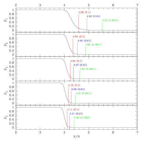
Figure 3: False alarm probability $P_{n}$ of having at least $n$ peaks caused by noise above a given signal-to-noise ratio (S/N) threshold in the Lomb-Scargle periodogram of KIC 08626021 (see text for details). In each panel, the 3 vertical lines indicate, from left to right, the S/N value corresponding to $P_{n}=0.1$, 0.01, and 0.0001, respectively. The limit $P_{1}=0.0001$, meaning that the risk of having a false detection above that threshold is reduced to less than 1 chance over 10 000, defines our adopted criterion. It corresponds to the limit of $5.6\sigma$.

Instead of adopting an arbitrary value, we quantitatively estimate what should be an acceptable threshold with the following procedure. Using the same time sampling as the observations, we randomly build 10 000 artificial lightcurves just containing white gaussian noise (a random normal deviate is calculated at each time point). The Lomb-Scargle Periodograms of these artificial lightcurves are then calculated, as well as the median values of the noise in each resulting LSPs. For any given S/N threshold ($x\sigma$ defined as $x$ times the median noise level) we then find the number of times that at least $n$ peaks in the LSP (which by definition are just noise structures) happen to be above the chosen limit. Then, dividing by the number of tests (10 000 here), we obtain the false alarm probability $P_{n}(x)$ that at least $n$ peaks above a given S/N threshold of $x\sigma$ is due to noise.

Figure 4: Lomb-Scargle Periodogram of the triplets at 4310 $\mu$Hz (up panel) and 5073 $\mu$Hz (bottom panel) after nearly two years of Kepler photometry gathered on KIC 08626021. The nearly equal frequency spacings are marked in the two panels. The dashed red horizontal line refers to the 5.6$\sigma$ detection threshold of local noise level.

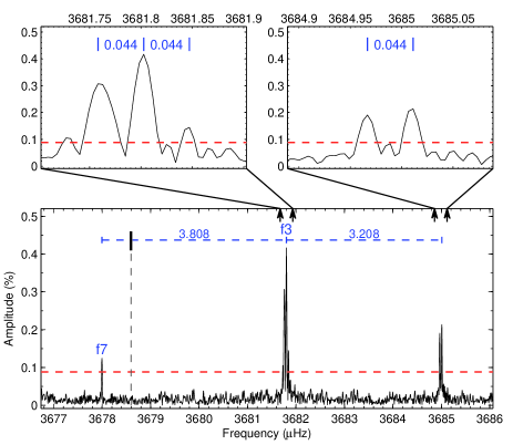
Figure 5: Lomb-Scargle Periodogram in the 3677$-$3686 $\mu$Hz frequency range where a doublet and a independent frequency are above the the 5.6$\sigma$ detection threshold of local noise level. The bold black vertical segment and vertical dashed line indicate the position of one possible third component for the doublet, as shown in the bottom panel. The two up panels are the expanded view of the two components as indicated by the vertical arrows in the bottom panel. Both the fine structures of the two components show well resolved closed peaks and share the same frequency separation of 0.044 $\mu$Hz.

Figure 3 shows the results of this procedure for the probabilities $P_{1}$ to $P_{5}$ as functions of the S/N threshold. The most interesting case is $P_{1}$ (the probability that at least 1 peak due to noise is above the threshold). We clearly see here that at the usual 4$\sigma$ limit, the probability to have at least one false detection is close to 1 (and $\sim 0.5$ to have at least 5 false detections according to $P_{5}$) confirming that this threshold is particularly unsafe in our case. However, $P_{1}$ eventually decreases with increasing S/N to reach 0.1 (10% chance) at S/N $\sim 4.58$, 0.01 (1% chance) at S/N $\sim 4.92$ (approximately the detection threshold chosen by BK14), and less than 1 chance out of 10 000 at S/N = 5.56 (this is the limit above which not a single peak due to noise has been found among the 10 000 randomly generated lightcurves).

Based on these calculations, we adopt in the following the conservative $5.6\sigma$ threshold as our limit of detection.

Table 1: List of frequencies detected in KIC 08626021.

Id.	Frequency	$\sigma_{f}$	Period	$\sigma_{P}$	Amplitude	$\sigma_{A}$	Phase	$\sigma_{\mathrm{Ph}}$	S/N	Comment
	($\mu$Hz)	($\mu$Hz)	(s)	(s)	(%)	(%)
$f_{1,-}$	4306.52304	0.00013	232.205886	0.000007	0.867	0.012	0.7987	0.0037	73.4	$f_{1,-}$ in BK14
$f_{1,0}$	4309.91490	0.00014	232.023143	0.000007	0.804	0.012	0.5264	0.0040	68.1	$f_{1,0}$ in BK14
$f_{1,+}$	4313.30642	0.00016	231.840705	0.000008	0.701	0.012	0.7885	0.0046	59.3	$f_{1,+}$ in BK14
$f_{2,-}$	5070.03081	0.00017	197.237460	0.000007	0.641	0.012	0.1521	0.0050	54.3	$f_{2,-}$ in BK14
$f_{2,0}$	5073.23411	0.00016	197.112922	0.000006	0.705	0.012	0.0394	0.0046	59.8	$f_{2,0}$ in BK14
$f_{2,+}$	5076.44385	0.00066	196.988291	0.000026	0.167	0.012	0.1462	0.0192	14.1	$f_{2,+}$ in BK14
$f_{3,0}$	3681.80286	0.00028	271.606068	0.000020	0.397	0.012	0.1347	0.0082	33.6	$f_{3,0}$ in BK14
$f_{3,+}$	3685.00937	0.00052	271.369731	0.000038	0.212	0.012	0.4066	0.0153	18.0	$f_{3,+}$ in BK14
$f_{4}$	2658.77740	0.00047	376.112721	0.000067	0.233	0.012	0.6147	0.0140	19.7	$f_{5}$ in BK14
$f_{5}$	4398.37230	0.00068	227.356834	0.000035	0.161	0.012	0.7598	0.0200	13.6	$f_{7}$ in BK14
$f_{6}$	3294.36928	0.00079	303.548241	0.000073	0.139	0.012	0.0934	0.0234	11.8	$f_{4,0}$ in BK14
$f_{7}$	3677.99373	0.00088	271.887358	0.000065	0.125	0.012	0.6773	0.0260	10.6	$f_{3,-}$ in BK14
$f_{9}$	6981.26129	0.00139	143.240592	0.000028	0.079	0.012	0.0105	0.0404	6.7	$f_{11}$ in BK14
Linear combination frequencies
$f_{8}$	6965.30234	0.00090	143.568786	0.000019	0.121	0.012	0.8358	0.0264	10.3	$f_{1,-}+f_{4}$ ; $f_{6}$ in O13
$f_{10}$	2667.95462	0.00164	374.818969	0.000230	0.067	0.012	0.7489	0.0484	5.7	$f_{9}-f_{1,+}$
Frequencies above 5 $\sigma$ detection
$f_{11}$	2676.38212	0.00170	373.638725	0.000236	0.065	0.012	0.1443	0.0501	5.5
$f_{12}$	3290.24565	0.00176	303.928675	0.000163	0.063	0.012	0.0752	0.0519	5.3	$f_{4,-}$ in BK14

2.3 Extraction of the frequencies

We used a dedicated software, FELIX (Frequency Extraction for LIghtcurve eXploitation) developed by one of us (S.C.), to first extract the frequency content of KIC 08626021 down to our adopted detection threshold of $5.6\sigma$ (we, in practice, pushed down the limit to $\sim 5\sigma$; see below). The method used is based on the standard prewhithening and nonlinear least square fitting techniques (Deeming, 1975) that works with no difficulty in the present case. The code FELIX greatly eases and accelerates the application of this procedure, especially for long and consecutive time series photometry obtained from spacecrafts like CoRoT and Kepler (Charpinet et al., 2010, 2011).

The list of extracted periodic signals is provided in Table 1 which gives their fitted attributes (frequency in $\mu$Hz, period in seconds, amplitude in % of the mean brightness, phase relative to a reference $t_{0}$ time, and signal-to-noise above the local median noise level) along with their respective error estimates ($\sigma_{f}$, $\sigma_{P}$, $\sigma_{A}$, and $\sigma_{\mathrm{Ph}}$). Figure 4, 5, and 6 show zoomed-in views of all the identified peaks in the Lomb-Scargle periodogram.

Figure 6: Lomb-Scargle Periodogram of 8 frequencies after nearly two years of Kepler photometry gathered on KIC 08626021. The two frequencies $f_{11}$ and $f_{12}$ are with 5.0$-$5.5 $\sigma$ of local noise level. Frequency $f_{8}$ and $f_{10}$ are linear combination frequencies.

We find 13 very clear independent frequencies that come out well above the detection threshold. Two additional lower amplitude peaks ($f_{8}$ and $f_{10}$) appear as significant but are linked to other frequencies through linear combinations and are therefore likely not independent pulsation modes. Two more frequencies ($f_{11}$ and $f_{12}$) can be identified above $5\sigma$ but below $5.6\sigma$ which we mention for completeness, but that cannot be considered as secured detections. A comparison with the completely independent analysis of BK14 shows that we agree on all the relevant, well secured frequencies (i.e, with a sufficiently high S/N ratio). We point out however that some additional features of the frequency spectrum are not discussed in BK14 and we differ on how to interpret some of the mode associations (see below).

As reported in BK14, six of the extracted frequencies ($f_{1}$ and $f_{2}$) form 2 very well defined, nearly symmetric triplets with a frequency spacing of $\sim 3.392$ $\mu$Hz and $\sim 3.206$ $\mu$Hz (Fig. 4). These are readily interpreted as rotationally split triplets, thus giving an average rotation period of $\sim 1.75$ day for the star. However, we argue that the 3 frequencies shown in Figure 5 cannot correspond to the components of a triplet, as BK14 suggest. These frequencies form a clearly asymmetric structure with the left component ($f_{7}$) being significantly more distant than the right component ($f_{3,+}$) from the central peak ($f_{3,0}$). We note in this context that the frequency separation between $f_{3,0}$ and $f_{3,+}$ ($3.208$ $\mu$Hz) is similar or very close to the frequency splitting characterizing the $f_{2}$ and $f_{1}$ triplets. Our interpretation is therefore that the middle ($f_{3,0}$) and right ($f_{3,+}$) peaks are 2 components of a triplet whose 3rd component is undetected, while the left peak ($f_{7}$) is a completely independent mode. This has some implications in finding an asteroseismic solution for KIC 08626021 as attempted by BK14, since 8 independent periods should be considered and not 7 (see Giammichele et al. 2015).

Furthermore, not reported in BK14, we show in Figure 5 that the two components of the incomplete triplet are in fact surrounded by additional structures (not tabulated in Table 1). The central peak ($f_{3,0}$) appears to have 2 resolved symmetric sidelobes located $0.044$ $\mu$Hz away, while the right peak ($f_{3,+}$) shows a sidelobe also separated by $0.044$ $\mu$Hz. These intriguing ”hyperfine” structures cannot be associated to rotation since a much larger rotational splitting signature has already been found. Moreover, the very small frequency separation involved would indicate a modulating phenomenon that occurs on a very long timescale of $\sim 263$ days.

This finding brings us to the main subject of the present paper, which is to show that this ”hyperfine” structure, along with other behaviors that we discuss below, can be linked to long term amplitude and frequency modulations generated by nonlinear resonant coupling mechanisms between the components of rotationally split triplets.

2.4 Amplitude and frequency modulations

From now on, we mainly focus our discussions on the two well defined triplets $f_{1}$ and $f_{2}$, and on the ”doublet” $f_{3}$ (i.e., the two visible components of an incomplete triplet). In order to analyze the time variability of these modes and their relationship, we used our software FELIX to compute the sliding Lomb-Scargle periodogram (sLSP) of the data set. This technique consists of building time-frequency diagrams by filtering in only parts of the data as a function of time. In the present case, we chose a filter window that is 180 day wide sled along the entire lightcurve by time steps of 7 days. This ensures a good compromise, for our purposes, between time resolution, frequency resolution (to resolve close structures in each LSP), and signal-to-noise. The sLSP gives an overall view of the amplitude and frequency variability that could occur for a given mode (see, e.g., the top left panel of Fig. 7). We acknowledge that BK14 also provide a similar analysis, but they chose a sliding window that is only 14 day wide, hence providing a much lower resolution in frequency. This has strong consequences on the interpretation of these data that will become obvious below. As a complementary (and more precise) method, we also extracted the frequencies (through prewithening and nonlinear least square fitting techniques) in various parts of the lightcurve, i.e., the 23-month light curve of KIC 08626021 was divided into 20 time intervals, each containing 6 months of data (for precision in the measurements) except for the last 3 intervals at the end of the observations. This second approach provides a measure of the (averaged) frequencies and amplitudes at a given time, along with the associated errors (see, e.g., the bottom left panel of Fig. 7).

2.4.1 The $f_{1}$ triplet

Figure 7 shows the amplitude and frequency modulations observed for the 3 components forming the $f_{1}$ triplet near 4310 $\mu$Hz. In this plot, views of the frequency variations with time are illustrated from top to bottom-left panels. The top panel first shows the sLSP of the triplet as a whole (similar to Figure 2 of BK14) where the signal appears, at this scale, stable in frequency but varying in amplitude for at least the central component. Then we provide increasingly expanded views (from middle-left to bottom-left panel) around the average frequency of each component. In addition, the bottom right panel shows how the amplitude of each component varies with time.

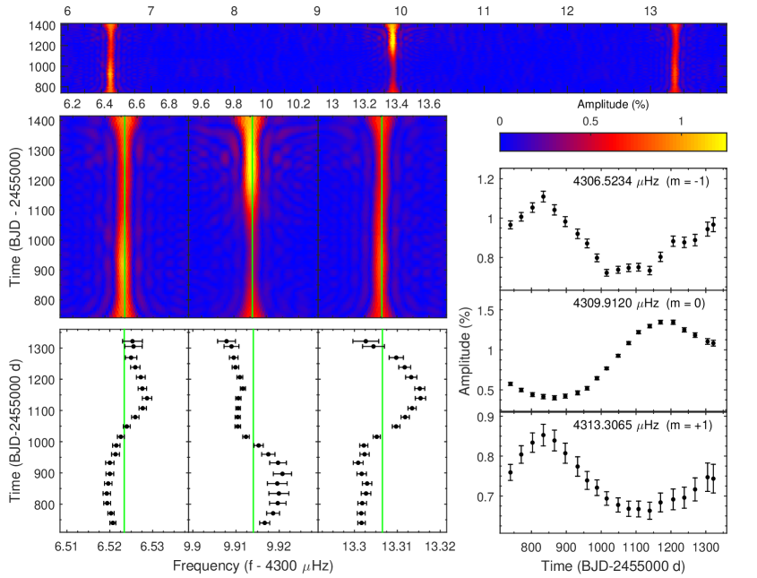
Figure 7: Frequency and amplitude modulations in the $f_{1}$ triplet at 4310 $\mu$Hz. The top panel shows the sliding Lomb-Scargle Periodogram (sLSP giving the amplitude in % as a function of frequency in $\mu$Hz and time in days) of the triplet as a whole. The middle and bottom left panels show increasingly expanded views around the average frequency (the solid vertical lines) of each component, with the bottom left panel obtained from prewhitening subsets of the data, thus measuring precisely the frequencies, as a function of time. The lower right panel provides the measured amplitudes as a function of time obtained for each subset of data (see text for details).

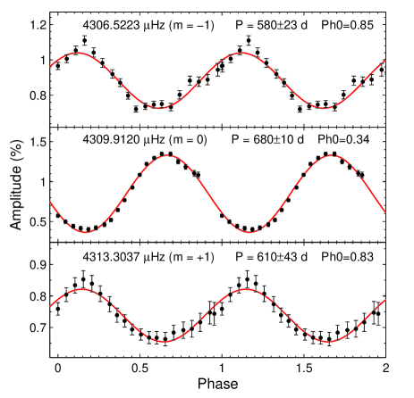
Figure 8: Amplitude modulations observed in the $f_{1}$ triplet presented in phase diagrams with a folding period of 580 and 610 days for the two side components, and 680 days for the central component. These periods, and their associated formal errors, were estimated by fitting a sinewave (red curve) to the amplitude variations.

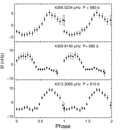
Figure 9: Same as Fig. 8 but for the frequency modulations observed in the $f_{1}$ triplet. Note that the folding periods adopted are the values derived for the corresponding amplitude modulations.

Figure 10: Same as Figure 7 but for the $f_{2}$ triplet at 5073 $\mu$Hz. Note that the component at 5076 $\mu$Hz has a very low amplitude and plunges below the 4 $\sigma$ detection threshold during the second half of the observations, making it difficult to follow (hence the 4 missing data points).

It is mentionned in BK14 that the modes, and these 3 components in particular, are stable in frequency over the 2-year duration of the observations. We clearly demonstrate here that this is not the case. Their statement is based on a time-frequency analysis involving a sliding Fourier Transform (sFT) that only uses a 14d-wide window, which clearly does not permit a sufficient frequency resolution to uncover the modulations that we report here. We find that both the amplitudes and frequencies show very suggestive signatures of quasi periodic modulations with an average timescale that we can roughly estimate to $\sim 620$ days. Figure 8 and 9 illustrate further this periodicity in phase diagrams. Although very similar, we find that the modulation period associated to the side components of the triplets ($\sim 600$ d) could be slightly shorter than the modulation period of the central component ($\sim 680$ d). Note that the modulating periods in this triplet were obtained by searching for the best fit of a pure sine wave function to the amplitude variations. The zero phase is relative to the time of the first data point (BJD=2 455 739.836). The same procedure was not applied to the frequency modulations since the patterns are clearly more complex than a pure sine wave function. However, since Fig. 7 suggests a cyclic behavior with roughly the same timescale, the folding periods used to construct Fig. 9 were chosen to be those derived for the amplitude modulations. This allows us to check that indeed at least two of the components (the $m=+1$ and $m=-1$ modes) accomodate rather well these periodicities, as the curves connect near phase 1. For the central ($m=0$) component, a slightly longer estimated periodicity does not permit to cover entirely the suspected modulation cycle with the data, leaving a gap between phase 0.9 and 1 where the behavior is not monitored. We cannot say in that case whether this curve would eventually connect smoothly at phase 1 or if a discontinuity exists, suggesting that either the chosen folding period is not appropriate or an additional trend is affecting the frequency of this mode.

In addition, we note that the frequency and amplitude modulations show obvious correlations, as both evolve in phase with the same period (with period of $\sim 600$ days and zero phase of $\sim 0.84$), for the side components, and are somewhat antiphased with the central component (with zero phase of $0.34$), as shown in Fig. 8 and 9. We quantitatively checked this fact by computing the correlation coefficients between, e.g., the amplitudes of the $m=+1$ and $m=-1$ components ($\rho_{A_{+},A_{-}}=+0.93$; i.e., indicative of a strong correlation) and the amplitudes of the $m=+1$ and $m=0$ components ($\rho_{A_{+},A_{0}}=-0.82$; i.e., indicative of a strong anti-correlation). Such correlated behavior suggests that the modes involved are somehow connected, either through a common cause affecting similarly their amplitude and frequency or through direct interactions occurring between the components of the triplet. This will be discussed further in Section 3.

2.4.2 The $f_{2}$ triplet

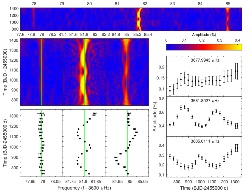
Figure 11: Same as Figure 7 but for the doublet $f_{3}$ at 3682 $\mu$Hz and the nearby independent frequency $f_{7}$ at 3678 $\mu$Hz.

Figure 10 shows the modulations observed in the other triplet, $f_{2}$, at 5073 $\mu$Hz. The frequencies in this triplet appear to be stable during the nearly two years of Kepler observations, while the amplitudes show clear modulations. Note that the amplitude of the $m=+1$ component went down at some point below a signal-to-noise ratio of $4\sigma$ and was essentially lost in the noise during a portion of the last half of the observations. Four measurements could not be obtained because of this and when it was still possible to spot this component, the errors remained large.

Again in this case, the amplitudes of the two side components seem to evolve nearly in phase with a quasi-periodic behavior on a timescale that is probably slightly larger than the duration of the observations and close to a timescale of $\sim 700$ day. However, contrary to the previous case, a connection with the central component is less clear. The later seems to follow a variation pattern possibly occurring on a longer time scale. Therefore, $f_{2}$ behaves somewhat differently from $f_{1}$, a feature that we will discuss more in the next section.

2.4.3 The $f_{3}$ doublet

The 3677$-$3686 $\mu$Hz frequency range is shown in Fig. 11 and contains the independent frequency ($f_{7}$) and the two visible components of the incomplete triplet $f_{3}$ (thus forming a doublet).

Each component of this doublet shows clear signatures of correlated variations for both amplitudes and frequencies. We note in particular a periodic modulation that occurs on a somewhat shorter timescale than for the two previous cases. A very quick look at Fig. 11 indicates a period of roughly 280 days for the amplitude variations of both modes as well as for the frequency modulation of $f_{3,0}$, which in fact can readily be connected to the ”hyperfine” structure sidelobes discussed in Section 2.3 and illustrated in Fig. 5. The frequency of $f_{3,+}$, for its part, seems to also follow a periodic trend but, quite interestingly, on a timescale that could be around twice ($\sim 550$ days) the period of the other components.

It appears now clearly that a periodic frequency and amplitude modulation process is responsible for the equidistant peaks surrounding $f_{3,0}$ and $f_{3,+}$. In this context, the 0.044 $\mu$Hz frequency separation should provide a more precise estimate of the period of this modulation, which is $\sim 263$ days. Note that the two other triplets discussed previously do not show similar ”hyperfine” splitting structures around their components simply because the period of their modulations appear to be slightly longer than the observational time baseline and those structures cannot be resolved. In the case of $f_{3}$, the observations are long enough to resolve the modulation. We further note that the amplitudes of the two components of $f_{3}$ evolves in antiphase while the frequencies are in phase during the first half of the run but then evolve in antiphase during the last part of the observations, which reflects the fact that the frequency variation of $f_{3,+}$ has approximately twice the period of the modulation seen in the frequency of $f_{3,0}$.

In contrast, the mode $f_{7}$ shows a totally different behavior as both its frequency and amplitude appear stable throughout the observing run. This could further support, if need be, the interpretation that $f_{7}$ and the $f_{3}$ complex are not part of a same triplet structure (as assumed by BK14). We indeed note that the theoretical framework in which these modulations can possibly be understood (nonlinear resonant couplings, as discussed in Section 3) forbids the possibility that the components of a triplet behave in different regimes.

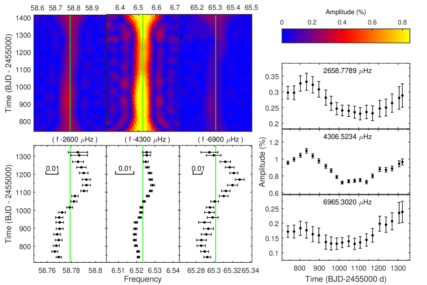
Figure 12: Frequency and amplitude modulations of the components forming the linear combination $f_{1,-}+f_{4}=f_{8}$. The panels are similar to those described in Figure 7. The three components show clear periodic modulations evolving in phase. In each bottom left subpanels, a segment indicates the 0.01 $\mu$Hz scale.

2.4.4 Other correlated modulations

For completeness, we also illustrate the interesting behavior of 3 frequencies related by a linear combination. Figure 12 shows the amplitude and frequency modulations of $f_{1,-}$, $f_{4}$ and $f_{8}$, that satisfy almost exactly (within $2\sigma$ of the formal measurement errors) the relation $f_{8}=f_{1,-}+f_{4}$ (see Table 1).

It is striking to see how the 3 components follow nearly exactly the same trends in both frequency and amplitude. These modulations could be related to the so called parents/child mode nonlinear interactions discussed by Breger & Montgomery (2014) or to other nonlinearities encountered in white dwarfs (e.g., Brassard et al. 1995; Wu 2001). In this context, we note, again according to the values given in Table 1, that the mean relative amplitude of $f_{8}$ ($A_{8}=0.00121$) is $\sim 60$ times larger than the product of the relative amplitudes of $f_{1,-}$ ($A_{1,-}=0.00867$) and $f_{4}$ ($A_{4}=0.00233$) whose value is $0.000020$. Figure 13 shows that these relationships also hold (within $2\sigma$), both for frequencies and amplitudes, for each individual measurement done as a function of time illustrated in Figure 12. Interestingly, if this combination were to be related to the mechanism of Wu (2001), the factor of $60$ connecting $A_{8}$ to $A_{1,-}.A_{4}$ would possibly imply that the inclination angle of the star should be $50^{\circ}<i<60^{\circ}$ (following Eqn. (20) in Wu 2001). Alternately, $f_{8}$ could result from a resonant mode coupling phenomenon where $f_{8}$ is a true eigenmode of the star (possibly of higher degree $\ell$) whose amplitude is boosted above the detection limit by the resonance following Eqn. (5) of Breger & Montgomery (2014, see also ). We indeed find that our results, instead of using phase (we here use frequency), are similar to the linear combination frequency families described in Breger & Montgomery (2014, e.g., comparing their Fig. 4-5 to our Fig. 13). However, at this stage, we cannot decipher which of these potential mechanisms could explain the details of this combination of frequencies due to the lack of further independent constraints (such as the inclination angle of KIC 08626021). Finally, we point out that one of the frequencies involved in this relation, $f_{1,-}$, is also involved as one of the components of the $f_{1}$ triplet discussed in Section 2.4.1 (and illustrated in Fig. 7).

Another similar linear combination has also been identified, involving $f_{1,+}$, $f_{9}$ and $f_{10}$, but the low amplitudes of $f_{9}$ and $f_{10}$ have prevented us from analyzing its frequency and amplitude modulations. In the following, we concentrate on a possible theoretical interpretation of the frequency and amplitude modulations observed in the triplets, and we do not discuss further the properties of linear combination frequencies.

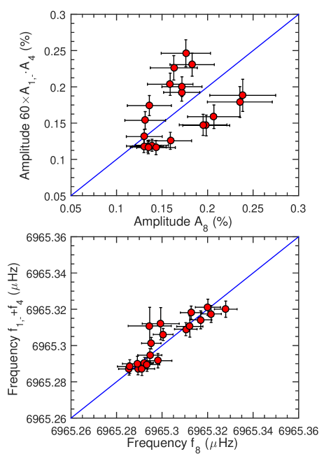
Figure 13: Top panel: Comparison between the measured amplitude $A_{8}$ of $f_{8}$ and 60 $\times$ $A_{1,-}\cdot{}A_{4}$ (where $A_{1,-}$ and $A_{4}$ are the amplitudes of $f_{1,-}$ and $f_{4}$, respectively) at each time segment (see text). Bottom panel: Same as top panel but for a comparison between the measured frequency $f_{8}$ and sum of the frequencies $f_{1,-}+f_{4}$. In both cases, the relationship is exactly statisfied along the plain diagonal line. All the measurements are found to be within $2\sigma$ of this line.

3 Links with nonlinear resonant couplings

The frequency and amplitude modulations observed in the two triplets and the doublet of KIC 08626021 cannot be related to any evolutionary effect, such as neutrino cooling, because the timescale involved is several orders of magnitude shorter than the cooling rate of DB white dwarfs (Winget et al., 2004). The signature of orbiting companions around the star is also ruled out by the fact that the variations occurring in different frequencies are not correlated in phase and do not have the same amplitude modulations (Silvotti et al., 2007). We also considered possibilities that instrumental modulations could occur, e.g., on a per quarter basis, such as a slightly varying contamination from the nearby star that could modulate the amplitude of the modes, but then all modes should be affected similarly, which is not what is observed. Finally, the possibility was raised that changes in the background state of the star, such as those induced by magnetic cycles or through an hypothetical angular momentum redistribution mechanism, could be responsible for the observed modulations. It is indeed well known that magnetic cycles have an impact on the frequencies of the $p$-modes observed in the Sun, leading to small frequency drifts that correlate well in time with tracers of the solar surface activity (see, e.g., Salabert et al. 2015 and references therein). One could imagine that such mechanisms may exist in white dwarfs as well. We find, however, that such effects would be hardly compatible with how the modes in KIC 08626021 are found to vary. In the Sun, all the modes appear to be globally affected following the same trends to some various extent, while in our case we see for instance a triplet $f_{1}$ that shows correlated changes in frequency, and at the same time another triplet $f_{2}$ whose frequencies appear to be constant. We find a mode $f_{7}$ that also does not change while the 2 visible components of the doublet $f_{3}$ nearby show correlated variations in frequency. This makes it difficult to connect these behaviors to a common global cause (i.e., small changes of the stellar structure). A cyclic redistribution of angular momentum, for its part, would affect the frequencies of the $m=+1$ and $m=-1$ components with an anti-correlation, while the central $m=0$ component should not be affected (and it is found to vary in $f_{1}$). All triplets should be affected nearly the same way, but $f_{2}$, showing constant frequencies, clearly is not and somewhat rules out this possibility.

Instead, we prefer to fall back to a simpler possibility. We develop in this section arguments that nonlinear resonant mode coupling mechanisms, by which both the amplitudes and frequencies of oscillation modes can be modulated on timescales of weeks, months, and even years, appears as a natural explanation for some of the observed behaviors.

3.1 The amplitude equations formalism

The amplitude equations (AEs) formalism is, to our knowledge, the only existing theoretical tool to investigate mode couplings for nonradial oscillation modes in pulsating stars. AEs in the stellar context have been extensively studied since the 1980’s for different types of couplings (Dziembowski, 1982; Buchler & Goupil, 1984; Moskalik, 1985; Dziembowski & Goode, 1992; Goupil & Buchler, 1994; van Hoolst, 1994; Buchler et al., 1995; Goupil et al., 1998; Wu, 2001; Wu & Goldreich, 2001).

In the present context, we limit ourselves to the type of resonances discussed in Buchler et al. (1995, 1997) and Goupil et al. (1998) involving linear frequency combinations such that $\nu_{1}\,+\nu_{2}\,\sim\,2\,\nu_{0}$, and, more specifically, a particular case in which a $\ell=1$ mode is split by slow rotation and form a nearly symmetric triplet. This choice is obviously driven by the specific configuration of the modes studied in KIC 08626021, which, we recall, are all identified as $\ell=1$ rotationally split $g$-mode triplets.

To clarify this further, we do not consider here other potential coupling mechanisms described, e.g., in Wu & Goldreich (2001) because they address a different problem, namely the problem of mode amplitude saturation through a proposed mechanism that indeed involves a nonlinear resonant mode coupling, but with one parent mode that is overstable (thus gaining energy) and two independent child modes that are damped (thus dissipating the energy). In our case, we observe and focus on a different nonlinear resonant coupling that occurs within triplets of l=1 $g$-modes resulting from the slow rotation of the star. The 3 modes in the triplets are overstable and nonlinearly interact with each other because slow rotation induces a near resonance relation between their frequencies (see below). Wu & Goldreich (2001), Wu (2001), Montgomery (2005), and other related studies do not treat this case and therefore cannot be helpful to describe and interpret what is occuring inside a rotationally split triplet. The only available framework for this is the Buchler et al. (1995, 1997) and Goupil et al. (1998) papers that explicitely developed a theory to describe this kind of interaction and that should not be confused we various other works on nonlinear interactions between modes. We point out that it does not mean that the Wu & Goldreich (2001) mechanism cannot also occur in KIC 08626021, but considering the linear growth rates expected for the observed modes (see Section 3.3 and Table 2), eventual limit cycles leading to cyclic amplitude variations would have timescales much longer ($\sim 1000$ yrs) than what is seen. This could hardly be connected to the observed features and would most likely not be noticeable in the available data that only cover a 2 year time baseline.

Going back to the configuration of interest involving rotationally split triplets, rotation treated to first order approximation would lead to a strictly symmetric triplet that exactly satisfies the above mentionned relationship. However, terms of higher order are never exactly zero and a small asymmetry, dominated by the second order term, always exists. This asymmetry is in fact essential for driving the various resonant coupling behaviors. The second order effect of rotational splitting, $\delta\nu_{t}$, that matters can be estimated following the equation given in Goupil et al. (1998):

$$\delta\nu_{t}=4C_{k\ell}\frac{\Omega^{2}}{\nu_{0}}$$ (1)

where $C_{k\ell}$ is the first order Ledoux constant ($\sim 0.5$ for dipole $g$-modes) and $\Omega\,=\,1/P_{rot}$ is the rotation frequency of the star. $P_{rot}$ is estimated from the first order average separation, $\Delta\nu$, between the components of the triplets and its value is $\sim 1.75$ days for KIC 08626021 (see Section 2). An asymmetry can also be evaluated directly from the measured frequencies of each triplet component, simply from the relation

$$\delta\nu_{o}=\nu_{-}+\nu_{+}-2\nu_{0}\qquad.$$ (2)

According to the resonant AEs from Buchler et al. (1995) in which they ignored the slight interactions between modes with different $\ell$ and $k$, for the components in the $\ell=1$ triplet with frequencies $\nu_{-}$, $\nu_{0}$ and $\nu_{+}$, the corresponding amplitudes $A_{-}$, $A_{0}$ and $A_{+}$ and phases $\phi_{-}$, $\phi_{0}$ and $\phi_{+}$ should obey the following relations

$$\frac{dA_{-}}{dt} =\kappa_{-}A_{-}+R_{-}A_{0}^{2}A_{+}\cos(\Phi-\delta_{-})$$

$$-A_{-}(q_{11}A_{-}^{2}+q_{12}A_{0}^{2}+q_{13}A_{+}^{2})$$ (3a)

$$\frac{dA_{0}}{dt} =\kappa_{0}A_{0}+R_{0}A_{0}A_{+}A_{-}\cos(\Phi+\delta_{0})$$

$$-A_{0}(q_{21}A_{-}^{2}+q_{22}A_{0}^{2}+q_{23}A_{+}^{2})$$ (3b)

$$\frac{dA_{+}}{dt} =\kappa_{+}A_{+}+R_{+}A_{0}^{2}A_{-}\cos(\Phi-\delta_{+})$$

$$-A_{+}(q_{31}A_{-}^{2}+q_{32}A_{0}^{2}+q_{33}A_{+}^{2})$$ (3c)

$$\frac{d\Phi}{dt} =\delta\nu-2R_{0}A_{-}A_{+}\sin(\Phi+\delta_{0})$$

$$+A_{0}(R_{-}\frac{A_{+}}{A_{-}}\sin(\Phi-\delta_{-})+R_{+}\frac{A_{-}}{A_{+}}\sin(\Phi-\delta_{+}))$$ (3d)

where $R_{-,0,+}$ and $q_{[(1,2,3)(1,2,3)]}$ are the nonlinear coupling coefficients associated to each component. Their values depend on complex integrals of the eigenfunctions of the modes involved in the coupling. The quantities $\kappa_{-}$, $\kappa_{0}$, and $\kappa_{+}$ are the linear growth rates of the $m=-1,0,+1$ components, respectively.

The numerical solutions of the AEs associated with this resonance identify three distinct regimes (see the example provided in Buchler et al., 1997). In order of magnitude, the occurrence of these three regimes can be roughly quantified by a parameter, $D$, defined as

$$D\equiv\frac{2\pi\delta\nu}{\kappa_{0}}.$$ (4)

But the ranges for this parameter defining the boundaries of the various regimes depends somewhat on the values of the nonlinear coefficients in the real star.

The first predicted situation is the nonlinear frequency lock regime in which the observed frequencies appear in exact resonance ($\delta\nu=0$) and the amplitudes are constant. In the case of the DB white dwarf star GD358, numerical solutions of the AEs indicated that the range of the $D$ parameter corresponding to this regime was between 0 and 20 (Goupil et al., 1998). However, these values are probably not universal and depend on the specific properties of the mode being considered, in particular on the value of the linear growth rate, $\kappa_{0}$, of the central component of the considered triplet.

When the triplet components move away from the resonance center ($\delta\nu\neq 0$), they enter the so-called intermediate regime where amplitude and frequency are no longer stable and modulations can appear in the pulsations. In this regime, periodic variations can be expected with a timescale of

$$P_{mod}\sim\frac{1}{\delta\nu}\simeq\frac{2\pi}{\kappa_{0}}\frac{1}{D}\qquad,$$ (5)

i.e., roughly the timescale derived from the inverse of the frequency asymmetry of the triplet (dominated by the second order effect of stellar rotation), which is connected to the inverse of the growth rate of the pulsating mode by the $D$ parameter (Goupil et al., 1998).

Far from the resonance condition, the modes recover the regime of steady pulsations with nonresonant frequencies. In the nonresonant regime, the nonlinear frequency shifts become very small and the frequencies are close to the linear ones.

We finally point out that in addition to the above three regimes, there exits a narrow hysteresis (transitory) regime between the frequency lock and intermediate regimes where the frequencies can be locked while the amplitudes still follow a modulated behavior.

3.2 Connection with the observed triplets

In light of the theoretical framework summarized above, we point out that some of the behaviors observed in the 2 triplets $f_{1}$ and $f_{2}$ and in the doublet $f_{3}$ (an incomplete triplet) can be quite clearly connected to nonlinear resonant couplings occurring in different regimes. We discuss each case below, but since the linear growth rate of the modes is an important ingredient to these resonance mechanism, we provide first some results of linear nonadiabatic pulsation calculations specifically tuned for a model representing best the DBV star KIC 08626021.

3.2.1 Nonadiabatic properties of the observed modes

Following our re-analysis of the data obtained for KIC 08626021 with Kepler, the recognition that 8 independent periods have to be considered for a detailed asteroseismic study (and not only 7 as used in BK14) coupled with our present need for a realistic seismic model representation of the star to carry out a nonadiabatic study of the mode properties led us to attempt a new asteroseismic analysis for this object. The details of this seismic study – a subject by its own that deserves a specific attention – are fully reported in Giammichele et al. (2015). The seismic solution obtained by Giammichele et al. (2015) for KIC 08626021 constitutes a major improvement over any of the fits proposed so far for this star, considering that it reproduces the 8 independent periodicities to the actual precision of the Kepler observations. It is therefore an excellent reference for our purposes.

We used this specific seismic model to estimate the theoretical linear growth rates of the fitted pulsations modes. These computations were done using two different nonadiabatic pulsation codes, one still working in the frozen convection (FC) approximation (Brassard et al., 1992; Fontaine et al., 1994; Brassard & Fontaine, 1997) and the other implementing a more realistic time-dependent convection (TDC) treatement (Dupret, 2001; Grigahcène et al., 2005). In DA and DB white dwarf pulsators, the superficial convection layer has an important contribution to the driving of modes (through the sometimes called convective driving mechanism). The positions of the theoretical instability strips, in particular the blue edges, are particularly sensitive to the adopted treatment (TDC vs FC) and to the efficiency of convection itself that controls the depths of the convection zone (the $\alpha$ parameter in the Mixing Length Theory; see Van Grootel et al., 2012). These can also affect the growth rate of each individual mode. Unfortunately, the oscillation periods have essentially no sensitivity to the $\alpha$ parameter, which is therefore not constrained by seismology. In this context, we explored various combinations of $\alpha$ values for the two different nonadiabatic treatments of the convection perturbation to estimate the typical range of values one would expect for the growth rate of the modes.

The results of these nonadiabatic calculations are summarized in Table 2 for the triplet (and doublet) components $f_{1}$, $f_{2}$, $f_{3}$, and, to be complete, for the other fitted frequencies as well. All these modes can effectively be driven in this star and the value of the growth rate $\kappa_{0}$ mostly depends on the radial order of the mode, strongly increasing when $k$ increases. For the modes of interest, we find that $\kappa_{0}$ lies in the ranges $2\cdot 10^{-13}-7\cdot 10^{-12}$, $2\cdot 10^{-12}-4\cdot 10^{-11}$, and $1\cdot 10^{-11}-2\cdot 10^{-10}$ for $f_{2}$, $f_{1}$, $f_{3}$, which, from the seismic solution of Giammichele et al. (2015), are successive dipole modes of radial order $k=3$, 4, and 5, respectively.

Table 2: Mode identification and linear non adiabatic growth rates, $\kappa_{0}$, from the best seismic model of KIC 08626021.

Id.	Frequency	$\ell$	$k$	$C_{k\ell}$	$\kappa_{0}^{\dagger}$	$\delta\nu_{t}$	$P_{m}$(th)	$\delta\nu_{o}$	$P_{m}$(obs)	$D$	Comment
	($\mu$Hz)					($\mu$Hz)	(day)	($\mu$Hz)	(day)
$f_{2,0}$	5073.23411	1	3	0.426	$2.10^{-13}-7.10^{-12}$	0.0148	780	0.0064	$\sim 700$	$1.10^{4}-5.10^{5}$	Hysteresis regime
$f_{1,0}$	4309.91490	1	4	0.456	$2.10^{-12}-4.10^{-11}$	0.0187	620	0.00034	$\sim 620$	$3.10^{3}-6.10^{4}$	Intermediate regime
$f_{3,0}$	3681.80287	1	5	0.469	$1.10^{-11}-2.10^{-10}$	0.0223	518	…	263	$7.10^{2}-1.10^{4}$	Intermediate regime
$f_{6}$	3294.36928	1	6	0.467	$2.10^{-11}-4.10^{-10}$	…	…	…	…	…
$f_{9}$	6981.26129	2	4	0.121	$7.10^{-12}-7.10^{-11}$	…	…	…	…	…
$f_{5}$	4398.37230	2	8	0.152	$4.10^{-10}-5.10^{-9}$	…	…	…	…	…
$f_{7}$	3677.99373	2	10	0.154	$2.10^{-9}-4.10^{-8}$	…	…	…	…	…
$f_{4}$	2658.77740	2	15	0.161	$1.10^{-7}-6.10^{-7}$	…	…	…	…	…

3.2.2 triplets in the intermediate regime

The periodic amplitude and frequency modulations observed in the triplet at 4310 $\mu$Hz ($f_{1}$) immediately suggest that this triplet is in the intermediate regime of the resonance (see again Fig. 7). Both the prograde and retrograde components show a modulation of frequency and amplitude with a period of $\sim$ 600 d. The central ($m=0$) component of $f_{1}$ has a frequency and amplitude modulation that is perhaps slightly longer ($\sim$ 680 d; precision is low here as this is about the same timescale as the duration of the observing campaign), but remains of the same order. For comparison purposes, we provide in Table 2 the modulation timescale $P_{m}(\rm th)\sim 1/\delta\nu_{t}$ (Eqn. 5) expected from the asymmetry, $\delta\nu_{t}$, caused by the second order correction to the rotational splitting. The latter is computed with the $C_{k\ell}$ value obtained from the reference model and the value $P_{\rm rot}=1.75$ days for the rotation period of the star. With $P_{m}(\rm th)\simeq 620$ days, the value obtained is sufficiently consistent with the observed modulation period to support the idea that we have indeed uncovered the right explanation for the behavior of the components in this triplet. Interestingly, the asymmetry can also be derived directly from the measured frequencies. Using directly the values given in Table 1, the quantity $\delta\nu_{o}$ represents the asymmetry for the frequencies averaged over the observation time baseline. We find it to be very small, i.e., much smaller than $\delta\nu_{t}$, suggesting that even in this intermediate regime the nonlinear interactions may already have forced the frequencies of the triplet components to a locked position (where $\delta\nu\rightarrow 0$), on average (since the frequencies are still varying with time, oscillating around their mean value).

According to the nonlinear resonant coupling theory, all the three components in a triplet should have the same modulations, both in amplitude and frequency. The slight difference between the side components and the central component in terms of the modulation period might be that the interaction of the modes in the DBV star is more complex than the idealized case described by the theory. It might also be a suggestion that the growth rates for each component of the triplet are not similar (as is assumed in this theoretical framework). The shape of the amplitude modulations of the retrograde component $f_{1,-}$ is not as smooth as the other two components. This might be caused by the additional coupling of the mode with $f_{4}$ at 2659 $\mu$Hz (see Section 2.4.4 and Figure 12). Such a coupling occurring outside the triplet is not considered by Buchler et al. (1995) who neglects other interactions with independent modes (i.e, the triplet is considered as an isolated system).

The second structure that can also be associated to the intermediate regime is the doublet $f_{3}$. We recall that the best interpretation for this doublet is that it belongs to a $\ell=1$ triplet with one of the side components (the low frequency one, $f_{3,-}$) missing, most likely because its amplitude is below the detection threshold. The two remaining components show clear periodic modulations of both frequencies and amplitudes. All variations occur on a somewhat shorter timescale of $P_{m}({\rm obs})\sim 263$ days (meaning that they are fully resolved in our data set, contrary to the modulations of $f_{1}$; see Section 2.4.3 and Fig. 11), except for the frequency of the $f_{3,-}$ component whose modulation period appear to be approximately twice that value ($P_{m}({\rm obs})\sim 550$ days). For this $f_{3}$ mode, the second order rotational splitting correction $\delta\nu_{t}$ also suggests a shorter modulation timescale of $P_{m}(\rm th)\sim 518$ days, which is comparable but not strictly identical. It is not possible in this case to evaluate $\delta\nu_{o}$ because of the missing third component.

3.2.3 A triplet in the transitory hysteresis regime

The case of the $f_{2}$ triplet at 5073 $\mu$Hz (see Section 2.4.2 and Figure 10) is slightly different in that the frequencies are clearly stabilized while the amplitudes are modulated. This suggests that $f_{2}$ is in another configuration, in between the frequency lock regime (where both amplitudes and frequencies are locked and therefore non-variable) and the intermediate regime. This configuration could be linked to the narrow transitory hysteresis regime briefly mentionned in section 3.1. This finding shows that two neighbor triplets can belong to different resonant regimes (frequency lock, narrow transition, intermediate or nonresonant), as it was also noticed for the white dwarf star GD 358 (Goupil et al., 1998).

3.3 Linear growth rates and the D parameter

Table 2 also provides the estimated values for the parameter $D$ derived from Eqn. (4) and from the values of $\delta\nu_{t}$ (Eqn. 1) and $\kappa_{O}$ (obtained from the seismic model of KIC 08626021; see Section 3.2.1). We find that $D$ lies in the ranges $3.10^{3}-6.10^{4}$, $1.10^{4}-5.10^{5}$ and $7.10^{2}-1.10^{4}$ for the triplets $f_{1}$, $f_{2}$ and $f_{3}$, respectively. These values are at least one order of magnitude larger than the range given in Goupil et al. (1998) for the intermediate regime ($D\sim 9-25$ for the white dwarf star GD 358). This large difference is clearly caused by the linear growth rates ($\kappa_{0}$) adopted for the modes. Our values come from a detailed linear nonadiabatic calculation based on the seismic model. Since the 3 triplets are fitted to low radial order consecutive modes ($k=3$, 4, and 5), their corresponding linear growth rates are generally small and differ substantially from one mode to the other ($\kappa_{0}$ increases rapidly with $k$). In contrast, Goupil et al. (1998) roughly scaled the growth rate of the modes according to the relationship $A_{k}^{2}/A^{2}_{k^{{}^{\prime}}}\sim\kappa_{k}/\kappa_{k}^{{}^{\prime}}$, assuming that all the coupling coefficients $q^{R}$ are of the same order of magnitude, leading to estimated values of $\kappa_{0}\sim 10^{-8}$. Values comparable to Goupil et al. (1998) for the growth rate could be obtained only if the 3 triplets were assigned to higher radial orders ($k$ between 10 and 15 instead of 3 to 5). This would require a huge shift compared to the current seismic solution which is clearly not permitted on the seismic modeling side.

In the AEs formalism of Buchler et al. (1997), the solutions admit three distinct regimes and one narrow transitory regime. Those regimes are related to the distance from the resonance center (i.e., $\delta\nu=0$). The parameter $D$ in this transitory regime should be slightly smaller than in the intermediate regime, as this transitory regime is closer to the resonance center. This means that $D$ should be smaller for $f_{2}$, which is in this transitory regime, compared to $f_{1}$ and $f_{3}$ that are in the intermediate regime. The ranges given for the $D$ values in Table 2 still permit this constraint to be roughly satisfied, but the overall larger $D$ values for $f_{2}$ could also lead to a contradiction here.

We think at this stage that further quantitative comparisons between theoretical considerations and the observed properties of the modulations would require to solve the amplitude equations specifically for this case. This is however beyond the scope of this paper, as no specific modeling tools for these nonlinear effects is available to us at present. We emphasize that with a detailed numerical solution of the nonlinear amplitude equations, the unknown coupling coefficients could, in principle, be determined from fitting the observed frequency and amplitude modulations. These coefficients, if known, would then allow us to derive the $D$ parameter which is strongly related to the different regimes of the nonlinear resonances. With the determination of this parameter, a measurement of the growth rate of the oscillation modes would then possibly follow, leading for the first time to an independent estimation of the linear nonadiabatic growth rates of the modes and a direct test of the nonadiabatic pulsation calculations.

4 Summary and conclusion

Frequency and amplitude modulations of oscillation modes have been found in several rotationally split triplets detected in the DB pulsator KIC 08626021, thanks to the high quality and long duration photometric data obtained with the Kepler spacecraft. These modulations show signatures pointing toward nonlinear resonant coupling mechanisms occurring between the triplet components. This is the first time that such signatures are identified so clearly in white dwarf pulsating stars, although hints of such effects had already been found from ground based campaigns in the past (e.g., Vauclair et al. 2011).

Reanalysing in detail the nearly 2 years of Kepler photometry obtained for this star, we have detected 13 very clear independent frequencies above our estimated ”secure” detection threshold ($5.6\sigma$; see Section 2.2 and Table 1), two frequencies that appear to be linear combinations of other independent modes, and two additional, but significantly less secured, frequencies emerging just above 5$\sigma$ the mean noise level. Overall, we find that our secured frequencies are consistant with those reported in BK14, but we somewhat differ on the interpretation of some structures in the frequency spectrum.

Most notably, we find that 3 frequencies in the 3677$-$3686 $\mu$Hz range, formerly identified as the components of a single triplet by BK14, cannot be interpreted like this. We conclude instead that one of the frequency ($f_{7}$ in Table 1) is an independent mode while the two others ($f_{3,0}$ and $f_{3,+}$) form the two visible components of an incomplete triplet whose third component is not seen. This has some implications for the seismic modeling which should in fact include 8 independent frequencies and not only 7 as in BK14. A new detailed seismic analysis of KIC 08626021 based on these 8 modes is provided by Giammichele et al. (2015). The frequency spacings (observed between the two components of $f_{3}$ and the components of two other well identified triplets, $f_{1}$ and $f_{2}$) indicate an average rotation period of $\sim 1.75$ days for KIC 08626021, i.e., in agreement with the value given by BK14.

Also differing from BK14, we find that the 2 components of the $f_{3}$ doublet have a ”hyperfine” structure with sidelobes separated by 0.044 $\mu$Hz, indicating a modulating phenomenon occurring on a long time scale of $\sim 263$ days. In addition, the components forming triplets show long term (quasi)-periodic frequency and/or amplitude modulations that appear to be correlated, as they evolve either in phase or antiphase. The triplet at 4310 $\mu$Hz ($f_{1}$) show signs of periodic modulation of both the frequencies and amplitudes with a timescale of roughly 600 days with the side components evolving in phase, while the central mode is in antiphase. The timescale appears somewhat shorter (263 days) for the $f_{3}$ doublet while the triplet $f_{2}$ shows only modulations in amplitudes (the frequencies appear stable during the observations) with a probable timescale of $\sim 700$ days.

We show that these behaviors can be related to the so-called nonlinear resonant coupling mechanisms that is expected to occur within rotationnally split triplets. The amplitude equations (Buchler et al., 1997; Goupil et al., 1998) predict 3 main regimes in which the triplet components may behave differently. It appears that $f_{1}$ and $f_{3}$ can be linked to the so-called intermediate regime of the resonance where both the amplitude and frequency of the modes should experience a periodic modulation. We find that the timescales expected from the theory are quite consistent with the observed periodicities of the modulations. The triplet $f_{2}$ shows a different behavior that can be associated with a narrow transitory hysteresis regime between the intermediate regime and the frequency locked regime in which locked frequencies and modulated amplitude solutions can coexist.

We also found correlated frequency and amplitude modulations in a linear combination of frequencies involving the modes $f_{1,-}$ and $f_{4}$, and the frequency $f_{8}$. This configuration may be related to parents/child mode interactions in pulsating stars, $f_{8}$ being either a combination frequency resulting from strong nonlinearities or, because the amplitude ratio is large, an eigenmode whose amplitude has been significantly enhanced by a resonant coupling phenomenon (see Breger & Montgomery 2014). Further investigations need to be carried out to evaluate which explanation is the most plausible.

As an additional step toward comparing more quantitatively observations to the theoretical expectations, we estimated theoretical linear growth rates (see Table 2) of the triplet central components using the seismic model provided by Giammichele et al. (2015). We used two different nonadiabatic pulsation codes for these computations: one working in the frozen convection approximation (Brassard et al., 1992; Fontaine et al., 1994; Brassard & Fontaine, 1997) and the other implementing a time-dependent convection treatement (Dupret, 2001; Grigahcène et al., 2005). The modes of interest $f_{2}$, $f_{1}$ and $f_{3}$ have growth rates that are in the ranges $2\cdot 10^{-13}-7\cdot 10^{-12}$, $2\cdot 10^{-12}-4\cdot 10^{-11}$, and $1\cdot 10^{-11}-2\cdot 10^{-10}$, respectively. With these values, we finally estimate the parameter $D$ (a key parameter that measures how far away is the mode from the resonance center) which is found in the range $3.10^{3}-6.10^{4}$, $1.10^{4}-5.10^{5}$ and $7.10^{2}-1.10^{4}$ for the mode triplet $f_{1}$, $f_{2}$ and $f_{3}$, respectively. These values are significantly larger than those estimated in Goupil et al. (1998) and need further investigation, but going beyond this would require to solve the amplitude equations for the specific case of KIC 08626021, which is currently not possible.

We want also to emphasize the fact that the uncovered frequency modulations, which are related to nonlinear coupling mechanisms and that occur on times scales long enough to be difficult to detect but short compared to the secular evolution timescale, can potentially impair any attempt to measure reliably the effects of the cooling of the white dwarf on the pulsation periods. Measuring the changing rate of the pulsation periods in white dwarf stars could indeed offer an opportunity to constrain the neutrino emission physics (Winget et al., 2004; Sullivan et al., 2008). However, one should be extremely careful of the potential contamination of nonlinear effects, which may need to be corrected first. Some independent modes in KIC 08626021 that seem to be stable in frequency over much longer timescales and that do not apparently couple with other modes in the white dwarf star could be good candidates for measuring period rates of change. But nonlinear interactions could still be affecting them on longer timescales that we cannot detect with Kepler.

Finally, the observed periodic frequency and amplitude modulations that occur in the intermediate regime of the resonance may allow for new asteroseismic diagnostics, providing in particular a way to measure for the first time linear growth rates of pulsation modes in white dwarf stars. This prospect should motivate further theoretical work on nonlinear resonant mode coupling physics and revive interest in nonlinear stellar pulsation theory in general.