GIANO-TNG spectroscopy of red supergiants in the young star cluster RSGC3

Abstract

Aims. The Scutum complex in the inner disk of the Galaxy has a number of young star clusters dominated by red supergiants that are heavily obscured by dust extinction and observable only at infrared wavelengths. These clusters are important tracers of the recent star formation and chemical enrichment history in the inner Galaxy.

Methods. During the technical commissioning and as a first science verification of the GIANO spectrograph at the Telescopio Nazionale Galileo, we secured high-resolution (R$\simeq$50,000) near-infrared spectra of five red supergiants in the young Scutum cluster RSGC3.

Results. Taking advantage of the full YJHK spectral coverage of GIANO in a single exposure, we were able to measure several tens of atomic and molecular lines that were suitable for determining chemical abundances. By means of spectral synthesis and line equivalent width measurements, we obtained abundances of Fe and iron-peak elements such as Ni, Cr, and Cu, alpha (O, Mg, Si, Ca, Ti), other light elements (C, N, F, Na, Al, and Sc), and some s-process elements (Y, Sr). We found average half-solar iron abundances and solar-scaled [X/Fe] abundance patterns for most of the elements, consistent with a thin-disk chemistry. We found depletion of [C/Fe] and enhancement of [N/Fe], consistent with standard CN burning, and low $\rm{}^{12}C/^{13}C$ abundance ratios (between 9 and 11), which require extra-mixing processes in the stellar interiors during the post-main sequence evolution. We also found local standard of rest V_LSR=106 km/s and heliocentric V_hel=90 km/s radial velocities with a dispersion of 2.3 km/s.

Conclusions. The inferred radial velocities, abundances, and abundance patterns of RSGC3 are very similar to those previously measured in the other two young clusters of the Scutum complex, RSGC1 and RSGC2, suggesting a common kinematics and chemistry within the Scutum complex.

1 Introduction

After RSGC1 (Figer et al., 2006) and RSGC2 (Davies et al., 2007), RSGC3 is the third young star cluster, to be rich in red supergiant (RSG) stars and located at the base of the Scutum-Crux arm (Clark et al., 2009; Alexander et al., 2009), at a distance of $\sim$3.5 kpc from the Galactic center.

These clusters host some tens of RSGs (with stellar masses of $\sim$14-20 $M_{\odot}$ and ages between 12 and 20 Myr) and have an estimated total mass of 2-4$\rm\times 10^{4}\leavevmode\nobreak\ M_{\odot}$. Some extended associations of RSGs have been also identified around them: Alicante 8, in the proximity of RSGC1 (Negueruela et al., 2010); Alicante 7 (Negueruela et al., 2011); and Alicante 10 (Gonzalez-Fernandez & Negueruela, 2012), have been associated with RSGC3. Davies et al. (2007) discussed the possibility that the Scutum complex is a giant star-forming region, where the activity is triggered by interactions with the Galactic bar, which is believed to end close to the base of the Scutum-Crux arm. Altogether, the Scutum complex provides a significant proportion of the known RSG population in the Galaxy.

The spectroscopic characterization of the chemical and kinematic properties of this region is still largely incomplete, given the prohibitive extinction ($A_{V}>$10 mag) that affects the Galactic plane at optical wavelengths, and observations can be performed mainly in the IR spectral domain.

Table 1: RSG stars in the star cluster RSGC3, observed with GIANO.

Ref	RA (J2000)	DEC (J2000)	SpT	J	H	K	Teff	AK	RVhel	RVLRS
S2	18 45 26.54	–03 23 35.3	M3Ia	8.53	6.62	5.75	3605	1.20	90	106
S3	18 45 24.34	–03 22 42.1	M4Ia	8.54	6.43	5.35	3535	1.47	86	102
S4	18 45 25.31	–03 23 01.1	M3Ia	8.42	6.39	5.31	3605	1.44	90	106
S5	18 45 23.26	–03 23 44.1	M2Ia	8.51	6.52	5.52	3660	1.43	92	108
S7	18 45 24.18	–03 23 47.3	M0Ia	9.12	6.97	6.20	3790	1.40	91	107

Note: Identification names, coordinates, spectral types, magnitudes, effective temperatures, reddening from Davies et al. (2009b); radial velocities (in the heliocentric and local standard of rest reference systems) in units of km/s from the GIANO spectra.

First radial velocity measurements have suggested that these young clusters and associations may share a common kinematics. For example, Davies et al. (2007) and Davies et al. (2008) derived average $v_{rad}$=+109 and +123 km/s for RSGC2 and RSGC1, respectively, from medium-high resolution K-band spectra of the CO bandheads. Negueruela et al. (2011) obtained average +102 and +95 km/s for RSGC2 and RSGC3, respectively, from their measurement of the Ca II triplet lines.

Some chemical abundances of Fe, C, O, and other alpha elements have been derived for stars in RSGC1 and RSGC2 (Davies et al., 2009b) by using NIRSPEC-Keck spectra at a resolution R$\approx$17,000. More recently, a few RSGs in RSGC2 and RSGC3 have been observed with GIANO, the new, cross-dispersed NIR spectrograph of the Telescopio Nazionale Galileo (TNG) at the Roque de Los Muchachos Observatory in La Palma (Spain) (see e.g. Oliva et al., 2012a, b, 2013; Origlia et al., 2014). More specifically, out of the targets observed during the commissioning runs to test the science performances of this new instrument, our group observed three bright red supergiants (RSGs) in the star cluster RSGC2 in July 2012 and five RSGs in the star cluster RSGC3 in October 2013. Chemical abundances for the stars in RSGC2 have already been published in Origlia et al. (2013). The chemical and kinematic analysis of the stars observed in RSGC3 is presented and discussed in this paper.

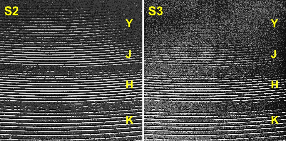
Figure 1: GIANO 2D (A-B) spectra of two observed RSGs in the RSGC3 star cluster.

2 Observations and data reduction

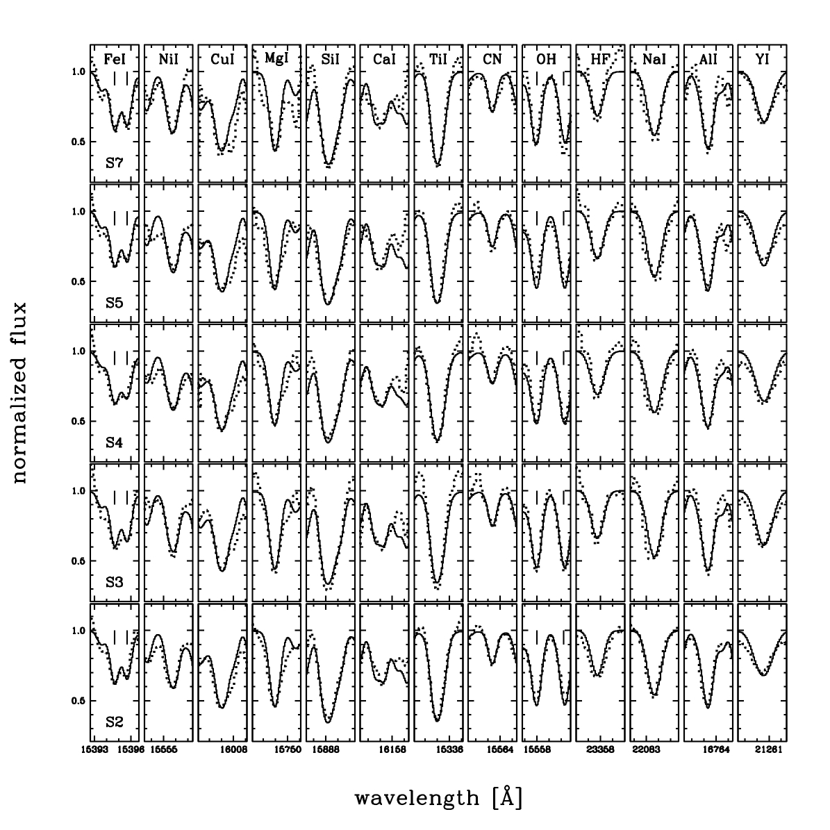
Figure 2: GIANO spectra around metal lines of interest for the five observed RSG stars (dotted lines). Our best-fit models are overplotted as solid lines. Rest frame wavelengths are defined in air and thickmarks represent every Å in each panel.

We used GIANO to observed five stars in RSGC3, S2, S3, S4, S5, and S7, from the list of Clark et al. (2009, see their Tables 1 and 2). For these RSGs they provided a spectral classification and a photometric estimate of the reddening and effective temperature that we list in Table 1. We note that the estimated reddening varies by large amounts (for example up to about two visual magnitudes between S2 and S3), even though the stars are clustered within a projected distance of about 1 arcmin (see e.g., Fig. 2 in Clark et al., 2009), which indicates that the cluster is both heavily and differentially obscured by foreground and/or local dust absorption.

The GIANO spectra of the RSGs in RSGC3 were collected during two technical nights in 2013 October 23 (star S2) and 27 (stars S3, S4, S5, and S7). GIANO is interfaced to the telescope with a couple of fibers mounted on the same connector at a fixed projected distance on sky of 3 arcsec. We observed the science targets by nodding on fiber, i.e. target and sky were taken in pairs and alternatively acquired on Fibers A and B, respectively, for an optimal subtraction of the detector noise and background. Two pairs of AB observations were performed for a total on-source integration time of 20 min.

An (A-B) 2D-spectrum was computed from each pair of exposures. Because of the image slicer, each 2D frame contains four tracks per order (two per fiber). Fig. 1 shows the (A-B) 2D echellograms of the S2 and S3 stars as an example. We note that significant continuum emission in the Y band has been detected only in star S2, the least reddened in the observed sample (see Table 1), while only a marginal detection has been obtained in the other stars.

In a single exposure, the 2D echellogram of GIANO covers the wavelength range from 0.95 $\mu$m to 2.4 $\mu$m at a resolving power R$\simeq$50,000, by spanning 49 orders from #32 to #80. The spectral coverage is complete up to 1.7 $\mu$m. At longer wavelengths, the orders become larger than the 2k $\times$ 2k detector. The effective spectral coverage in the K-band is about 75%.

To extract and perform the wavelength calibration of the echelle orders from the 2D GIANO spectra, we used the ECHELLE package in IRAF and some new, ad hoc scripts grouped in a package called GIANO_TOOLS that can be retrieved from the TNG WEB page (http://www.tng.iac.es/instruments/giano/giano_tools_v1.2.0.tar.gz). We used 2D spectra of a tungsten calibration lamp taken in daytime to map the geometry of the four spectra in each order and for flat-field purposes. A U-Ne lamp spectrum at the beginning and/or end of each observing night was used for wavelength calibration. We selected about 30 bright lines (mostly Ne lines) distributed over a few orders to obtain a first fit, then the optimal wavelength solution was computed by using about 300 U-Ne lines that were distributed over all orders, with a typical accuracy of 300 m/s throughout the entire echellogram. The positive (A) and negative (B) spectra of the target stars were extracted and added together to get a 1D wavelength-calibrated spectrum with the best possible signal-to-noise ratio (S/N).

3 Spectral analysis and chemical abundances

From the observed GIANO spectra, we were able to provide radial velocity measurements of the observed RSGs (see Table 1), finding average V_LSR=106 km/s and heliocentric V_hel=90 km/s values with a dispersion of 2.3 km/s, which is fully consistent with the stars being members of the RSGC3 cluster and the Scutum complex (see, e.g., Davies et al., 2007, 2008; Negueruela et al., 2011).

The chemical abundances were measured as in Origlia et al. (2013) for the red supergiants in RSGC2. We used an updated version (Origlia, Rich & Castro, 2002) of the code, as first described in Origlia, Moorwood & Oliva (1993), to model RSG spectra by varying the stellar parameters and the element abundances. The code uses the LTE approximation and is based on both the molecular-blanketed model atmospheres of Johnson, Bernat & Krupp (1980), at temperatures $\leq$4000 K, and on the ATLAS9 models for temperatures above 4000 K.

The NIR continuum opacity in cool giant and supergiant star atmospheres is mostly set by the H^- ion, and therefore it is most important to secure a correct molecular blanketing to define the temperature structure when computing these model atmospheres. Metal abundances are much less critical in defining such an opacity for the continuum (see also Rich & Origlia, 2005).

The code also includes thousands of NIR atomic transitions from the Kurucz database, Biemont & Grevesse (1973), and Melendez & Barbuy (1999), while molecular data are taken from our own (Origlia, Moorwood & Oliva, 1993, and subsequent updates) and B. Plez (private communications) compilations. Hyperfine structure splitting has been accounted for in the Ni, Sc, and Cu line profile computations, although including them does not significantly affect the abundance estimates. The reference solar abundances are taken from Grevesse & Sauval (1998).

As discussed in Origlia et al. (2013), deriving chemical abundances in RSGs is not trivial. We used full spectral synthesis and equivalent-width measurements of selected lines, which are free from significant blending and/or contamination by telluric absorption, and which do not have strong wings. Our best-fit solution is the one that minimizes the scatter between observed and synthetic spectra, in terms of both line equivalent width and overall spectral synthesis around the lines of interest.

A first compilation of suitable lines at high spectral resolution in the NIR, on which to perform abundance analysis in RSGCs, can be found in Origlia et al. (2013). For the RSGs in RSGC3, we were also able to infer some Cu abundances from the measurement of the neutral line at $\lambda$=16006.5 Å (log gf=+0.25, $\chi$=5.35 eV), not included in the list by Origlia et al. (2013). The presence of possible telluric absorption around each line was carefully checked on an almost featureless O-star (Hip103087) spectrum.

The high spectral resolution and the many CO, OH, and CN molecular lines, as well as the neutral atomic lines available in the GIANO spectra, allowed us to constrain the atmospheric parameters and the spectral broadening quite strictly because of both micro and macro turbulence. We obtained a good fit to the observed spectra of the RSGC3 stars by adopting i) a stellar temperature T$\approx$3600 K for all the stars except S7, for which we used T$\approx$3800 K, which is in perfect agreement with the photometric values reported in Table 1; ii) log g=0.0 for the gravity; iii) a value of 3 km/s for the microturbulence velocity; and iv) macroturbulence velocity with a Gaussian $\sigma$ broadening of about 6 km/s, or the equivalent of a Doppler-broadening of 8-9 km/s. We did not find any other appreciable line broadening by stellar rotation.

Microturbulence velocity in cool giants and supergiants can be constrained at the level of 0.5-1.0 km/s (also depending on the S/N of the spectra) from the shape of the ¹²CO bandheads. Microturbulence does not change the depth of the bandheads significantly, it only broadens them.

As already discussed in Origlia et al. (2013) for the measured RSGs in RSGC2, the observed line profiles in the GIANO spectra of the RSGs in RSGC3 are definitely broader than the instrumental one (as determined from telluric lines and from the GIANO spectra of standard stars). This type of extra-broadening is likely due to macroturbulence and is normally modeled in the same way as the instrumental profile by assuming it is Gaussian. The inferred velocities are in the range of values (from several to a few tens of km/s) measured, e.g., in the RSGs of the Galactic center (Ramirez et al., 2000; Cunha et al., 2007; Davies et al., 2009a).

At the GIANO spectral resolution of 50,000, we find that variations of $\pm$100K in T_eff, $\pm$0.5 in log g and $\pm$0.5 km/s in microturbulence have effects on the spectral lines that can also be noticed by visual inspection, and therefore we consider them representative of the systematic uncertainties. Variations in temperature, gravity, and microturbulence that are smaller than the above values are difficult to disentangle because of the limited sensitivity of the lines and the degeneracy among stellar parameters. Moreover, this kind of finer tuning would have a negligible impact on the inferred abundances (less than a few hundreths of a dex, i.e. smaller than the measurement errors). The impact of using slightly different assumptions for the stellar parameters on the derived abundances is discussed in Sect. 3.1.

We could estimate the chemical abundances of Fe, Ni, Cu, Mg, Si, Ca, Ti, Na, Al, Sc, and yttrium from the equivalent width measurements of neutral atomic lines in the H and K-bands. Additional abundances of Cr, Sr, and potassium have only been measured in S2, the least reddenend star, by using lines in the Y and J bands. The Y- and J-band spectra of the other stars do not have enough S/N to obtain reliable equivalent width measurements. Equivalent width measurements of the OH and CN molecular lines in the H-band, and of one HF line in the K-band, were used to determine the oxygen, nitrogen, and fluorine abundances. With regard to the latter, we first estimated the F abundances using the HF(1-0) R9 line parameters from Cunha et al. (2003), as done in Origlia et al. (2013). However, Jönsson et al. (2014) have very recently revised the line parameters (see also Jorissen, Smith & Lambert, 1992), and we also computed the F abundances using these new values The two abundance determinations differ on average by $\sim$0.2 dex, the higher abundances being obtained with the old values from Cunha et al. (2003). Figure 2 shows examples of the spectral lines observed with GIANO from which metals abundances have been derived.

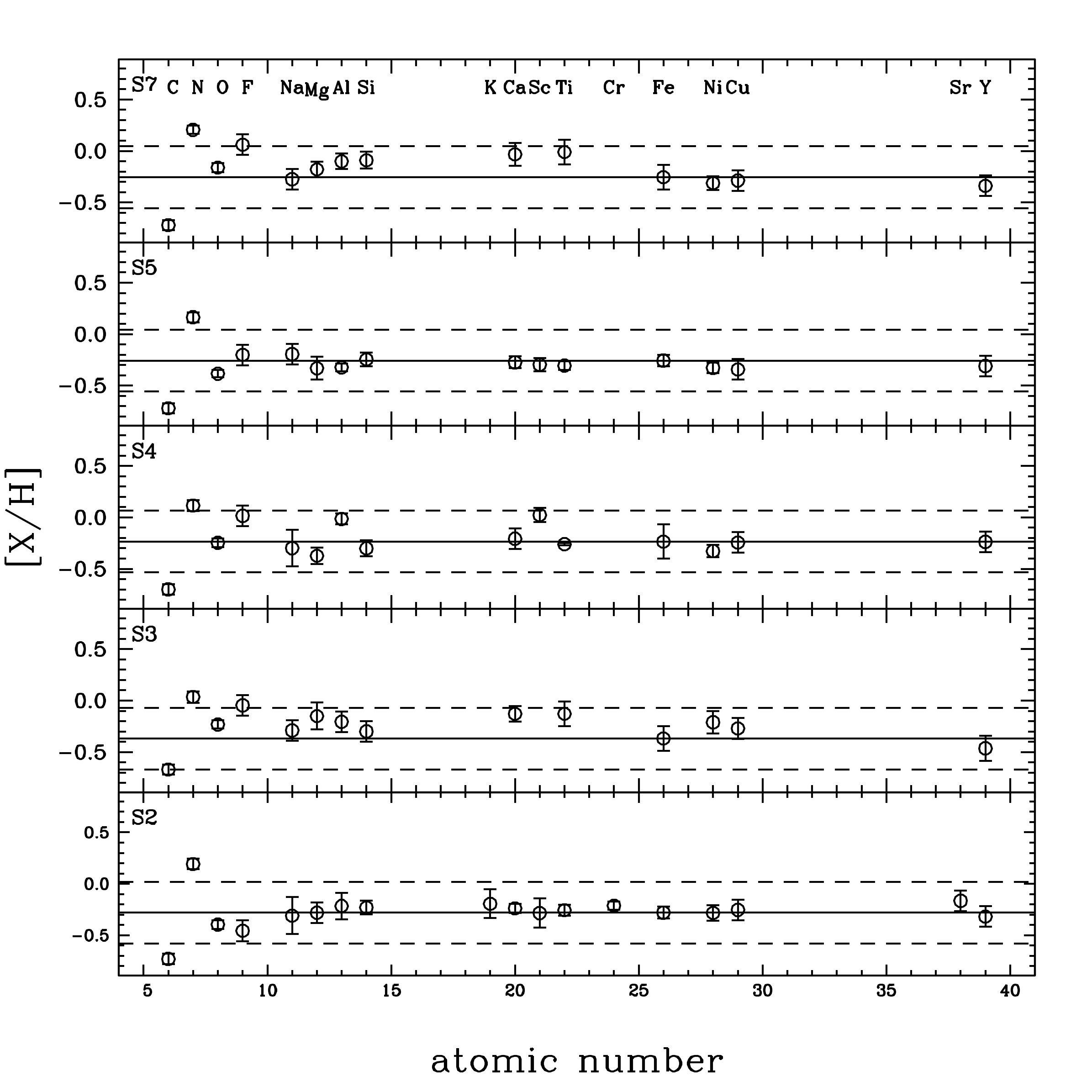
Figure 4: [X/H] chemical abundances as a function of the atomic number for the five RSGs in the star cluster RSGC3, as observed with GIANO. The horizontal lines indicate the [Fe/H] abundance (solid) and the $\pm$0.3 dex values (dashed), as inferred in the present analysis.

The ¹²C and ¹³C carbon abundances were mostly determined from the CO bandheads in the H- and K-bands, respectively, using full spectral synthesis because of the high level of crowding and blending of the CO lines in these stars. Figure 3 shows the GIANO spectra of the five RSGs centered on some of the CO bandheads used to determine the abundance. The average metal abundances for the sampled chemical species are quoted in Table 2 and plotted in Fig. 4.

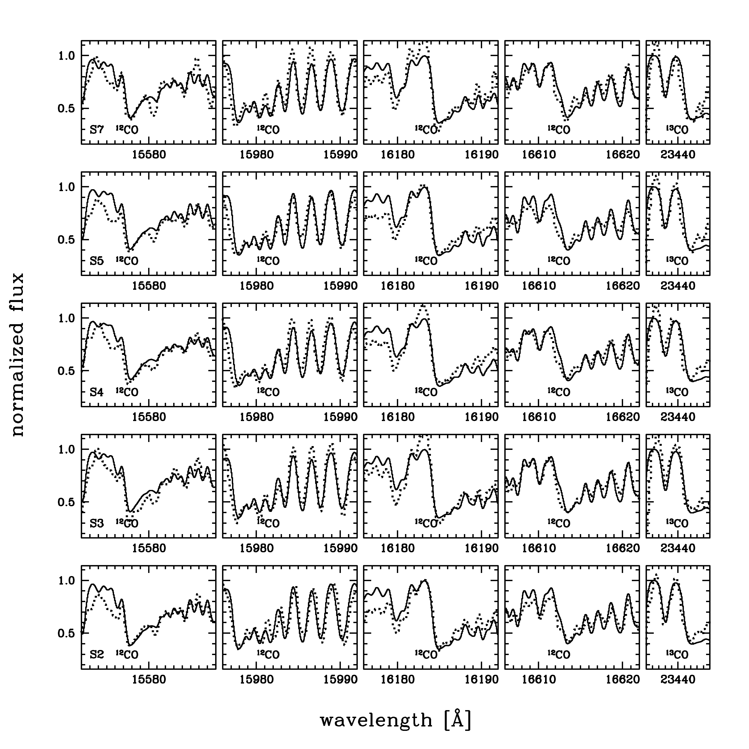
Figure 3: GIANO H-band spectra of the ¹²CO (3-0), (5-2), (6-3) and (8-5) bandheads and K-band spectra of the ¹³CO (2-0) bandhead for the five observed RSG stars (dotted lines). Our best-fit models are overplotted as solid lines. Rest frame wavelengths are defined in air and thickmarks represent every Å in each panel.

3.1 Error budget

The typical random error of the measured line equivalent widths is between 10 and 20 mÅ, mostly the result of a $\pm$2% uncertainty in the placement of the pseudocontinuum, as estimated by overlapping the synthetic and the observed spectra. This error corresponds to abundance variations ranging from a few hundredths to one-tenth of a dex and is lower than the typical 1$\sigma$ scatter ($\leq$0.15 dex) in the derived abundances from different lines. The errors for the final abundances quoted in Table 2 were obtained by dividing these 1$\sigma$ errors by the squared root of the number of used lines, typically a few in the case of atomic lines, and 10-20 in the case of the CN and OH molecular lines. When only one line was available, we assumed a 0.1 dex error.

As detailed in Origlia et al. (2013), a somewhat conservative estimate of the overall systematic uncertainty in the abundance (X) determination, which is caused by variations of the atmospheric parameters, can be computed with the following formula: $\rm(\Delta X)^{2}=(\partial X/\partial T)^{2}(\Delta T)^{2}+(\partial X/\partial log\leavevmode\nobreak\ g)^{2}(\Delta log\leavevmode\nobreak\ g)^{2}+(\partial X/\partial\xi)^{2}(\Delta\xi)^{2}$. We computed test models with variations of $\pm$100 K in temperature, $\pm$0.5 dex in log g, and $\pm$0.5 km/s in microturbulence velocity with respect to the best-fit parameters, and we found that these systematic uncertainties in stellar parameters can impact the overall abundances at a level of 0.15-0.20 dex.

As in Origlia et al. (2013), we also determined the statistical significance of our best-fit solution for the spectral synthesis of the CO features and the derived carbon abundances. As a figure of merit of the statistical test, we adopted the difference between the model and the observed spectrum. To quantify systematic discrepancies, this parameter is more powerful than the classical $\chi^{2}$ test, which instead is equally sensitive to random and systematic deviations (see Origlia & Rich, 2004, for more discussion and references).

Our best-fit solutions always show $>$90% probability of being representative of the observed spectra, while solutions with $\pm$0.1 dex abundance variations or with $\rm\Delta T=\pm$100 K, $\rm\Delta log\leavevmode\nobreak\ g=\pm$0.5 dex, and $\rm\Delta\xi=\pm$0.5 km s^-1, as well as corresponding simultaneous variations in the C abundance (0.1-0.2 dex) to reproduce the depth of the molecular features, are statistically significant only at 1-2$\sigma$ level.

As discussed in Davies et al. (2013) (see also Levesque et al., 2005) significantly different temperatures can be inferred using different scales. This issue has been explored by extensive simulations in Origlia et al. (2013) for the three studied RSGs in RSGC2, and finding that, when temperatures were both significantly warmer and cooler than those that provide the best fit solutions, one can barely fit the observed spectra except with very peculiar CNO abundance patterns. We repeated the same tests for the five RSGs analyzed here and reached very similar conclusions.

Table 2: Chemical abundances of the RSG stars in the star cluster RSGC3 observed with GIANO.

Ela	[X/H]b
	S2	S3	S4	S5	S7
Fe (26)	-0.28 (12)	-0.37 (5)	-0.23 (4)	-0.26 (11)	-0.25 (4)
	$\pm$ 0.06	$\pm$ 0.12	$\pm$ 0.17	$\pm$ 0.06	$\pm$ 0.12
Cr (24)	-0.21 (5)	–	–	–	–
	$\pm$ 0.04	–	–	–	–
Ni (28)	-0.28 (6)	-0.21 (5)	-0.33 (6)	-0.33 (4)	-0.31 (7)
	$\pm$ 0.07	$\pm$ 0.11	$\pm$ 0.06	$\pm$ 0.05	$\pm$ 0.07
Cu (29)	-0.25 (1)	-0.27 (1)	-0.24 (1)	-0.34 (1)	-0.29 (1)
	$\pm$ 0.10	$\pm$ 0.10	$\pm$ 0.10	$\pm$ 0.10	$\pm$ 0.10
Mg (12)	-0.28 (4)	-0.15 (4)	-0.37 (3)	-0.33 (4)	-0.18 (3)
	$\pm$ 0.10	$\pm$ 0.13	$\pm$ 0.08	$\pm$ 0.11	$\pm$ 0.07
Si (14)	-0.23 (5)	-0.30 (1)	-0.30 (3)	-0.25 (3)	-0.09 (2)
	$\pm$ 0.07	$\pm$ 0.10	$\pm$ 0.08	$\pm$ 0.07	$\pm$ 0.08
Ca (20)	-0.24 (5)	-0.13 (4)	-0.21 (4)	-0.27 (5)	-0.03 (4)
	$\pm$ 0.05	$\pm$ 0.08	$\pm$ 0.10	$\pm$ 0.06	$\pm$ 0.11
Ti (22)	-0.26 (16)	-0.13 (3)	-0.26 (3)	-0.31 (8)	-0.01 (3)
	$\pm$ 0.05	$\pm$ 0.12	$\pm$ 0.01	$\pm$ 0.04	$\pm$ 0.12
C (6)	-0.73	-0.67	-0.70	-0.72	-0.62
	$\pm$ 0.05	$\pm$ 0.05	$\pm$ 0.05	$\pm$ 0.05	$\pm$ 0.05
N (7)	0.19 (13)	0.04 (9)	0.12 (12)	0.16 (12)	0.21 (14)
	$\pm$ 0.05	$\pm$ 0.06	$\pm$ 0.05	$\pm$ 0.05	$\pm$ 0.04
O (8)	-0.40 (9)	-0.23 (16)	-0.25 (17)	-0.38 (13)	-0.16 (19)
	$\pm$ 0.04	$\pm$ 0.04	$\pm$ 0.04	$\pm$ 0.03	$\pm$ 0.05
Fc (9)	-0.46 (1)	-0.05 (1)	0.02 (1)	-0.20 (1)	0.06 (1)
	$\pm$ 0.10	$\pm$ 0.10	$\pm$ 0.10	$\pm$ 0.10	$\pm$ 0.10
Na (11)	-0.31 (2)	-0.29 (1)	-0.30 (2)	-0.19 (1)	-0.27 (1)
	$\pm$ 0.18	$\pm$ 0.10	$\pm$ 0.18	$\pm$ 0.10	$\pm$ 0.10
Al (13)	-0.22 (3)	-0.21 (1)	-0.01 (3)	-0.32 (3)	-0.10 (2)
	$\pm$ 0.13	$\pm$ 0.10	$\pm$ 0.05	$\pm$ 0.04	$\pm$ 0.08
K (19)	-0.19 (2)	–	–	–	–
	$\pm$ 0.14	–	–	–	–
Sc (21)	-0.28 (3)	–	0.02 (2)	-0.30 (2)	–
	$\pm$ 0.14	–	$\pm$ 0.07	$\pm$ 0.06	–
Sr (38)	-0.16 (1)	–	–	–	–
	$\pm$ 0.10	–	–	–	–
Y (39)	-0.32 (1)	-0.46 (2)	-0.24 (1)	-0.31 (1)	-0.34 (1)
	$\pm$ 0.10	$\pm$ 0.12	$\pm$ 0.10	$\pm$ 0.10	$\pm$ 0.10
$\rm{}^{12}C/^{13}C$	11$\pm 1$	11$\pm 1$	10$\pm 1$	9$\pm 1$	10$\pm 1$

^a Chemical element and corresponding atomic number in parenthesis.

^b Numbers in parenthesis refer to the number of lines used to compute the abundances.

^c F abundances are obtained from the HF(1-0) R9 line using the parameters listed in Jönsson et al. (2014).

4 Discussion and conclusions

Red supergiants are very luminous NIR sources even in highly reddened environments, such as the inner Galaxy, and they can be spectroscopically studied at high resolution even with 4m-class telescopes, provided that these are equipped with efficient cross-dispersed spectrographs like GIANO. Indeed, the simultaneous access to the YJHK bands provided by GIANO offers the possibility of sampling most of the chemical elements of interest and to measure from a few to several tens of lines per element, thus enabling an accurate and statistically significant abundance analysis.

All five RSGs observed in RSGC3 show similar iron abundances, further confirming their likely membership in the cluster. We found average half-solar iron and iron-peak (Ni and Cu) abundances and solar-scaled [X/Fe] abundance ratios (with r.m.s $<0.1$ dex) for the measured s process (yttrium in all the five stars and Sr in only star S2), alpha, and other light elements, but carbon, nitrogen and, to a lower level, fluorine. Abundance ratios of [C/Fe] and [N/Fe] are depleted and enhanced, respectively, by a similar factor (between two and three), and the resulting [(C+N)/Fe] and [(C+N+O)/Fe] average abundance ratios turn out to be about zero with rms of 0.09 and 0.19 dex, respectively, which is consistent with standard CNO nucleosynthesis. We also found low $\rm{}^{12}C/^{13}C$ ratios (between 9 and 11). As suggested by Davies et al. (2009b) and also mentioned in Origlia et al. (2013) rotationally enhanced mixing (e.g., Meynet & Maeder, 2000) can account for both the overall depletion of carbon and the low $\rm{}^{12}C/^{13}C$ isotopic ratio in RSGs. In this respect, it is interesting to note that measurements of the $\rm{}^{12}C/^{13}C$ ratio in the interstellar medium (Milam et al., 2005) suggest a value of $\sim 33$ at a Galactocentric distance of 3.5 kpc. [F/Fe] and [F/O] are slightly enhanced (by about 0.15 dex), which is consistent with measurements in RSGC2 (Origlia et al., 2013) and in the Orion Nebula Cluster (Cunha & Smith, 2005).

Mild abundance ratio enhancement (at a level of $\sim$0.2 dex) of [Mg/Fe] in star S3, of [Ca/Fe] and [Ti/Fe] in stars S3 and S7, and of [Al/Fe] and [Sc/Fe] in star S4 has been measured. In the least reddened star S2, we also measured [K/Fe] and [Sr/Fe] abundance ratios. These are only slightly enhanced (by 0.1 dex), but are still consistent with solar-scaled values within the errors.

These abundances and abundance patterns are fully consistent with those measured in RSGC1 and RSGC2 (Davies et al., 2009b; Origlia et al., 2013), and suggest a rather homogeneous kinematics and chemistry within the Scutum complex, as traced by its young populations of RSGs. Their slightly sub-solar metallicity is intriguing, as already mentioned in Origlia et al. (2013), since both measurements of Cepheids (see e.g. Genovali et al., 2013; Andrievsky et al., 2013, and references therein) and open clusters (see e.g. Magrini et al., 2009), as well as model predictions (see e.g. Cescutti et al., 2007), suggest metal abundances that are well in excess of solar at larger Galactocentric distances ($\geq$4 kpc). In this respect, however, it is interesting to note that the RSGs in the Galactic center (about solar, Ramirez et al., 2000; Cunha et al., 2007; Davies et al., 2009a; Ryde & Schultheis, 2015) do not also reach these high metal abundances, thus suggesting that the chemical enrichment in the innermost regions of the Galaxy is more complicated and deviates from the metallicity gradient observed in the outer disk. The about solar-scaled metal abundances of alpha and other light elements, similar to those measured in the thin disk (see e.g.. Reddy et al., 2003), indicate an enrichment by both type II and type I supernovae on long timescales.

Taken together, these first NIR spectroscopic studies at medium-high resolution of the chemical and kinematic properties of the young stellar populations in the inner Galaxy reveal their potential astrophysical impact in complementing the information derived from the older and fainter population of giant stars in less obscured regions. Indeed, a proper characterization of the chemical enrichment of the various stellar populations across the entire disk is critical for a comprehensive reconstruction of its formation and evolution history.

Finally, it is worth noting that these high-resolution studies of RSGs in the Galaxy and in the Magellanic Clouds are also crucial for better interpreting the low resolution and/or integrated spectral information of these young stellar populations in distant star-forming galaxies.