Curvature of the pseudocritical line in (2+1)-flavor QCD with HISQ fermions

Abstract:

We study QCD with (2+1)-HISQ fermions at nonzero temperature and nonzero imaginary baryon chemical potential. Monte Carlo simulations are performed using the MILC code along the line of constant physics with a light to strange mass ratio of $m_{l}/m_{s}=1/20$ on lattices up to $48^{3}\times 12$ to check for finite cutoff effects. We determine the curvature of the pseudocritical line extrapolated to the continuum limit.

1 Introduction

Quantum ChromoDynamics (QCD) is widely accepted as the theory of strong interactions and, as such, must encode all the information needed to precisely draw the phase diagram in the temperature ($T$) - barion chemical potential $(\mu_{B})$-plane. As a matter of fact, only some corners of it can be accessed by first-principle applications of QCD, in the perturbative or in the nonperturbative regime. The region of the phase diagram where $\mu_{B}/(3T)\lesssim 1$ is within the reach of the lattice approach of QCD and one can therefore address, at least inside this region, the problem of determining the shape taken by the QCD pseudocritical line separating the hadronic from the deconfined phase. There is no a priori argument for the coincidence of the QCD pseudocritical line with the chemical freeze-out curve: if the deconfined phase is realized in the fireball, in cooling down the system first re-hadronizes, then reaches the chemical freeze-out. This implies that the freeze-out curve lies below the pseudocritical line in the $\mu_{B}$-$T$ plane. It is a common working hypothesis that the delay between chemical freeze-out and rehadronization is so short that the two curves lie close to each other and can therefore be compared. Under the assumptions of charge-conjugation invariance at $\mu_{B}=0$ and analyticity around this point, the QCD pseudocritical line, as well as the freeze-out curve, can be parameterized, at low baryon densities, by a lowest-order Taylor expansion in the baryon chemical potential, as

$$\frac{T(\mu_{B})}{T_{c}(0)}=1-\kappa\left(\frac{\mu_{B}}{T(\mu_{B})}\right)^{2}\;,$$ (1)

where $T_{c}(0)$ and $\kappa$ are, respectively, the pseudocritical temperature and the curvature at vanishing baryon density.

As is well known direct Monte Carlo simulations of lattice QCD at nonzero baryon density are hindered by the well known “sign problem”: $S_{E}$ becomes complex and the Boltzmann weight loses its sense. Several ways out of this problem have been devised (see Ref. [1, 2, 3, 4] for a review). In the present work we use the approach of analytic continuation from imaginary chemical potential. Our aim is to determine the continuum limit of the curvature $\kappa$ of the pseudocritical line of QCD with nf =2+1 staggered fermions at nonzero temperature and quark density. More details are reported in Ref. [5].

The state-of-the-art of lattice determinations of the curvature $\kappa$, up to the very recent papers of Ref. [6, 7], is summarized in Fig. 10 of Ref. [8]: depending on the lattice setup and on the observable used to probe the transition, the value of $\kappa$ can change even by almost a factor of three. The lattice setup dependence stems from the kind of adopted discretization, the lattice size, the choice of quark masses and chemical potentials, the procedure to circumvent the sign problem. On the side of the determinations of the freeze-out curve, two recent determinations [9, 10] of $\kappa$, both based on the thermal-statistical model, but the latter of them including the effect of inelastic collisions after freeze-out, give two quite different values of $\kappa$, each seeming to prefer a different subset of lattice results (see Fig. 3 of Ref. [11] for a snapshot of the situation).

2 Numerical results

We perform simulations of lattice QCD with 2+1 flavors of rooted staggered quarks at imaginary quark chemical potential. We have made use of the HISQ/tree action [12, 13, 14] as implemented in the publicly available MILC code [15], which has been suitably modified by us in order to introduce an imaginary quark chemical potential $\mu=\mu_{B}/3$. In the present study we put $\mu=\mu_{l}=\mu_{s}$, with $\mu_{l}$ the light quark chemical potential and $\mu_{s}$ the strange quark chemical potential. This means that the Euclidean partition function of the discretized theory reads

$$Z=\int[DU]e^{-S_{\rm gauge}}\prod_{q=u,d,s}{\rm det}(D_{q}[U,\mu])^{1/4}\;,$$ (2)

where $S_{\rm gauge}$ is the Symanzik-improved gauge action and $D_{q}[U,\mu]$ is the staggered Dirac operator, modified for the inclusion of the imaginary quark chemical (see Ref. [13] and appendix A of Ref. [14] for the precise definition of the gauge action and the covariant derivative for highly improved staggered fermions).

We have simulated the theory at finite temperature, and for several values of the imaginary quark chemical potential, near the transition temperature, adopting lattices of size $16^{3}\times 6$, $24^{3}\times 6$, $32^{3}\times 8$, $40^{3}\times 10$ and $48^{3}\times 12$. All simulations make use of the rational hybrid Monte Carlo (RHMC) algorithm. The length of each RHMC trajectory has been set to $1.0$ in molecular dynamics time units. We have discarded typically not less than one thousand trajectories for each run and have collected from 4k to 8k trajectories for measurements.

The pseudocritical point $\beta_{c}(\mu^{2})$ has been determined as the value for which the renormalized disconnected susceptibility of the light quark chiral condensate divided by $T^{2}$ exhibits a peak.
The bare disconnected susceptibility is given by:

$$\chi_{l,\rm disc}={{n_{f}^{2}}\over 16L_{s}^{3}L_{t}}\left\{\langle\bigl{(}{\rm Tr}D_{q}^{-1}\bigr{)}^{2}\rangle-\langle{\rm Tr}D_{q}^{-1}\rangle^{2}\right\}\;,$$ (3)

Here $n_{f}=2$ is the number of light flavors and $L_{s}$ denotes the lattice size in the space direction. The renormalized chiral susceptibility is defined as:

$$\chi_{l,\rm ren}=\frac{1}{Z_{m}^{2}}\;\chi_{l,\rm disc}.$$ (4)

The multiplicative renormalization factor $Z_{m}$ can be deduced from an analysis of the line of constant physics for the light quark masses. More precisely, we have [14]:

$$Z_{m}(\beta)\;=\;\frac{m_{l}(\beta)}{m_{l}(\beta^{*})}\;,$$ (5)

where the renormalization point $\beta^{*}$ is chosen such that:

$$\frac{r_{1}}{a(\beta^{*})}\;=\;2.37\;,$$ (6)

where the function $a(\beta)$ is discussed below.

To precisely localize the peak in $\chi_{l,\rm ren}/T^{2}$, a Lorentzian fit has been used. For illustrative purposes, in Fig. 1 we display our determination of the pseudocritical couplings at $\mu/(\pi T)=0.2i$ for all lattices considered in this work.

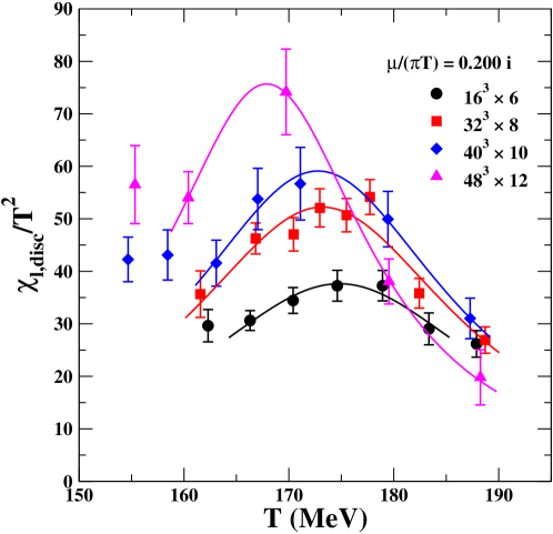
Figure 1: The real part of the renormalized susceptibility of the light quark chiral condensate over $T^{2}$ on the lattices $16^{3}\times 6$, $32^{3}\times 8$, $40^{3}\times 10$ and $48^{3}\times 12$ at $\mu/(\pi T)=0.2i$. Full lines give the Lorentzian fits near the peaks.

To get the ratios $T_{c}(\mu)/T_{c}(0)$, we fix the lattice spacing through the observables $r_{1}$ and $f_{K}$, following the discussion in the Appendix B of Ref. [16].
For the $r_{1}$ scale the lattice spacing is given in terms of the $r_{1}$ parameter as:

$$\frac{a}{r_{1}}(\beta)_{m_{l}=0.05m_{s}}=\frac{c_{0}f(\beta)+c_{2}(10/\beta)f^{3}(\beta)}{1+d_{2}(10/\beta)f^{2}(\beta)}\;,$$ (7)

with $c_{0}=44.06$, $c_{2}=272102$, $d_{2}=4281$, $r_{1}=0.3106(20)\ {\text{fm}}$.
On the other hand, in the case of the $f_{K}$ scale we have:

$$af_{K}(\beta)_{m_{l}=0.05m_{s}}=\frac{c_{0}^{K}f(\beta)+c_{2}^{K}(10/\beta)f^{3}(\beta)}{1+d_{2}^{K}(10/\beta)f^{2}(\beta)}\;,$$ (8)

with $c_{0}^{K}=7.66$, $c_{2}^{K}=32911$, $d_{2}^{K}=2388$, $r_{1}f_{K}\simeq 0.1738$. In Eqs. (7) and (8), $f(\beta)$ is the two-loop beta function,

$$f(\beta)=(b_{0}(10/\beta))^{-b_{1}/(2b_{0}^{2})}\exp(-\beta/(20b_{0}))\;,$$ (9)

$b_{0}$ and $b_{1}$ being its universal coefficients.

For all lattice sizes the behavior of $T_{c}(\mu)/T_{c}(0)$ can be nicely fitted with a linear function in $\mu^{2}$,

$$\frac{T_{c}(\mu)}{T_{c}(0)}=1+R_{q}\left(\frac{i\mu}{\pi T_{c}(\mu)}\right)^{2}\;,$$ (10)

which gives us access to the curvature $R_{q}$ and, hence, to the curvature parameter $\kappa=-R_{q}/(9\pi^{2})$ introduced in Eq. (1). On the $24^{3}\times 6$ lattice the linearity in $\mu^{2}$ has been assumed to hold, in order to extract $R_{q}$ from the only available determination at $\mu/(\pi T)=0.2i$.

For the sake of the extrapolation to the continuum limit, in Fig. 2 we report our determinations of $R_{q}$ on the lattices $24^{3}\times 6$, $32^{3}\times 8$, $40^{3}\times 10$, $48^{3}\times 12$, and from the two different methods to set the scale, versus $1/L_{t}^{2}$.

Within our accuracy, cutoff effects on $R_{q}$ are negligible, so that a constant fit works well over the whole region ($\chi^{2}_{r}\simeq 0.99$), thus including also the smallest $24^{3}\times 6$ lattice. Taking into account the uncertainties due to the continuum limit extrapolation,

$$\kappa=0.020(4)\;.$$ (11)

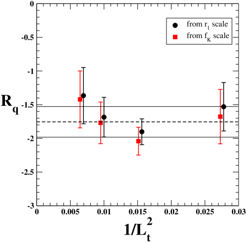
Figure 2: Determinations of the curvature $R_{q}$ on the lattices $24^{3}\times 6$, $32^{3}\times 8$, $40^{3}\times 10$, $48^{3}\times 12$, and from the two different methods to set the scale, versus $1/L_{t}^{2}$. The dashed horizontal line gives the result of the fit to all data with a constant; the solid horizontal lines indicate the uncertainty on this constant.

Therefore we can conclude that, within the accuracy of our determinations, cutoff effects on the curvature are negligible already on the lattice with temporal size $L_{t}=6$. Our determination of the curvature parameter, $\kappa$=0.020(4), is indeed compatible with the value quoted in our previous paper [11], $\kappa$=0.018(4), without the extrapolation to the continuum.

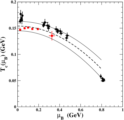
Figure 3: $T_{c}(\mu_{B})$ versus $\mu_{B}$ (units in GeV). Experimental values of $T_{c}(\mu_{B})$ are taken from Fig. 1 of Ref. [9] (black circles) and from Fig. 3 of Ref. [17] (green triangles), for the standard hadronization model and for the susceptibilities of conserved charges respectively. The dashed line is a parametrization corresponding to $T_{c}(\mu_{B})=T_{c}(0)-b\mu_{B}^{2}$ with $T_{c}(0)=0.154(9)\,\text{GeV}$ and $b=0.128(25)\,{\text{GeV}}^{-1}$ . The solid lines represent the corresponding error band.

Finally it is interesting to extrapolate the critical line as determined in this work to the region of real baryon density and compare it with the freeze-out curves resulting from a few phenomenological analyses of relativistic heavy-ion collisions. This is done in Fig. 3, where we report two different estimates. The first is from the analysis of Ref. [9], based on the standard statistical hadronization model, where the freeze-out curve is parametrized as

$$T_{c}(\mu_{B})=a-b\mu_{B}^{2}-c\mu_{B}^{4}\;,$$ (12)

with $a=0.166(2)\ {\text{GeV}}$, $b=0.139(16)\ {\text{GeV}}^{-1}$, and $c=0.053(21)\ {\text{GeV}}^{-3}$. The second estimate is from Ref. [17] and is based on the analysis of susceptibilities of the (conserved) baryon and electric charges. In fact, our critical line is in nice agreement with all the freeze-out points of Refs. [9, 17]. In particular, using our estimate of the curvature, Eq. (11), we get $b=0.128(25)\ {\text{GeV}}^{-1}$, in very good agreement with the quoted phenomenological value.

Some caveats are in order here. We do not expect our critical line to be reliable too far from $\mu=0$: as a rule of thumb, we can trust it up to real quark chemical potentials of the same order of the modulus of the largest imaginary chemical potential included in the fit (10), i.e. $|\mu|/(\pi T)=0.25$. This translates to real baryon chemical potentials in the region $\mu_{B}/T\lesssim 0.25$. Moreover, the effect of taking $\mu_{s}=\mu_{l}$ instead of $\mu_{s}<\mu_{l}$ should become visible on the shape of the critical line as we move away from $\mu=0$ in the region of real baryon densities, thus reducing further the region of reliability of our critical line. So, from a prudential point of view, the agreement shown in Fig. 3 could be considered the fortunate combination of different kinds of systematic effects. We cannot however exclude the possibility that the message from Fig. 3 is to be interpreted in positive sense, i.e. the setup we adopted and the observable we considered may catch better some features of the crossover transition, thus explaining the nice comparison with freeze-out data. Indeed, our result for the continuum extrapolation of the curvature $\kappa$ is in fair agreements with the recent estimates in Ref. [6], where both setup $\mu_{s}=\mu_{l}$ and $\mu_{s}=0$ were adopted, and Ref. [7], where the strangeness neutral trajectories were determined from lattice simulations by imposing $\langle n_{S}\rangle=0$.

References

- [1] O. Philipsen, The QCD phase diagram at zero and small baryon density, PoS LAT2005 (2006) 016, [hep-lat/0510077].
- [2] C. Schmidt, Lattice QCD at finite density, PoS LAT2006 (2006) 021, [hep-lat/0610116].
- [3] P. de Forcrand, Simulating QCD at finite density, PoS LAT2009 (2009) 010, [arXiv:1005.0539].
- [4] G. Aarts, Complex Langevin dynamics and other approaches at finite chemical potential, PoS LATTICE2012 (2012) 017, [arXiv:1302.3028].
- [5] P. Cea, L. Cosmai, and A. Papa, The continuum limit of the critical line of 2+1 flavor QCD, arXiv:1508.07599.
- [6] C. Bonati, M. D’Elia, M. Mariti, M. Mesiti, F. Negro, and F. Sanfilippo, Curvature of the chiral pseudo-critical line in QCD: continuum extrapolated results, arXiv:1507.03571.
- [7] R. Bellwied, S. Borsanyi, Z. Fodor, J. Günther, S. D. Katz, C. Ratti, and K. K. Szabo, The QCD phase diagram from analytic continuation, arXiv:1507.07510.
- [8] C. Bonati, M. D’Elia, M. Mariti, M. Mesiti, F. Negro, et al., Curvature of the chiral pseudocritical line in QCD, Phys.Rev. D90 (2014), no. 11 114025, [arXiv:1410.5758].
- [9] J. Cleymans, H. Oeschler, K. Redlich, and S. Wheaton, Comparison of chemical freeze-out criteria in heavy-ion collisions, Phys.Rev. C73 (2006) 034905, [hep-ph/0511094].
- [10] F. Becattini, M. Bleicher, T. Kollegger, T. Schuster, J. Steinheimer, et al., Hadron Formation in Relativistic Nuclear Collisions and the QCD Phase Diagram, Phys.Rev.Lett. 111 (2013) 082302, [arXiv:1212.2431].
- [11] P. Cea, L. Cosmai, and A. Papa, Critical line of 2+1 flavor QCD, Phys.Rev. D89 (2014), no. 7 074512, [arXiv:1403.0821].
- [12] HPQCD Collaboration, UKQCD Collaboration Collaboration, E. Follana et al., Highly improved staggered quarks on the lattice, with applications to charm physics, Phys.Rev. D75 (2007) 054502, [hep-lat/0610092].
- [13] MILC Collaboration, A. Bazavov et al., Nonperturbative QCD simulations with 2+1 flavors of improved staggered quarks, Rev.Mod.Phys. 82 (2010) 1349–1417, [arXiv:0903.3598].
- [14] MILC collaboration Collaboration, A. Bazavov et al., Scaling studies of QCD with the dynamical HISQ action, Phys.Rev. D82 (2010) 074501, [arXiv:1004.0342].
- [15] http://physics.utah.edu/~detar/milc.html.
- [16] A. Bazavov, T. Bhattacharya, M. Cheng, C. DeTar, H. Ding, et al., The chiral and deconfinement aspects of the QCD transition, Phys.Rev. D85 (2012) 054503, [arXiv:1111.1710].
- [17] P. Alba, W. Alberico, R. Bellwied, M. Bluhm, V. Mantovani Sarti, et al., Freeze-out conditions from net-proton and net-charge fluctuations at RHIC, Phys.Lett. B738 (2014) 305–310, [arXiv:1403.4903].