Atomically thin spherical shell-shaped superscatterers based on Bohr model

Abstract

Graphene monolayers can be used for atomically thin three-dimensional shell-shaped superscatterer designs. Due to the excitation of the first-order resonance of transverse magnetic (TM) graphene plasmons, the scattering cross section of the bare subwavelength dielectric particle is enhanced significantly by five orders of magnitude. The superscattering phenomenon can be intuitively understood and interpreted with Bohr model. Besides, based on the analysis of Bohr model, it is shown that contrary to the TM case, superscattering is hard to occur by exciting the resonance of transverse electric (TE) graphene plasmons due to their poor field confinements.

I Introduction

With the concept of metamaterials and metasurfaces, subwavelength structures can demonstrate unusual electromagnetic properties nmat11-917 ; LPR9-195 , e.g. surface plasmons in coaxial metamaterial cables JOSAB27-148 ; MPLB27-1330013 and graphene-based cloaks acsnano5-5855 ; OE21-12592 ; JP27-185304 . Specially, the scattering of subwavelength structures can be enhanced to realize superscatterers, which can magnify the scattering cross section of a given object remarkably OE16-18545 . Due to their potential applications in detection, spectroscopy, and photovoltaics PNAS ; JPCC ; APL73-3815 ; NL8-3983 ; prl90-057401 ; JAP101-093105 ; nmat9-205 , various superscatterers with different shapes and types have been designed NJP10-113016 ; APL94-223513 ; NJP11-073033 ; OE18-6891 ; CMS49-820 ; JOSAA30-1698 ; PRL105-013901 ; APL98-043101 ; prl108-083902 ; PRA86-033825 ; OE21-10454 ; APL105-011109 ; JPCC118-30170 ; nanoscale6-9093 , and the concept of superscatterer has been extended to acoustics APA99-843 ; FP7-319 .

Superscatterer was first proposed in the framework of transformation optics, where both electric and magnetic anisotropic inhomogeneous materials were needed OE16-18545 . In order to loose the requirement, Ruan and Fan PRL105-013901 ; APL98-043101 proposed a kind of subwavelength superscatterer by engineering an overlap of resonances of different plasmonic modes where they only use multilayered isotropic plasmonic structures. To extend their superscatterer into the deep-subwavelength scale, we put forward the idea of using graphene monolayer to realize cylindrical superscatterers with the advantage of active tunability OL40-1651 . Since graphene is a two dimensional carbon sheet with only one atom thick RMP ; science332-1291 , this superscatterer can be treated as one kind of “surface superscatterers”. However, in practical applications, three dimensional (3D) superscatterers are more promising since the objects to be superscattered are usually 3D. Different from the two dimensional (2D) cylindrical case, the parallel polarized and vertically polarized fields cannot been decoupled from the incident electromagnetic field in the 3D case. Thus, it is desirable to extend the notion of “superscattering by a surface” to the 3D case.

Furthermore, similarities between quantum physics and wave optics have been hot topics in recent decades bookQCA ; LPR3-243 . On one hand, optics provides a fertile ground to simulate some basic concepts in quantum mechanics and quantum field theory, such as PT symmetry prl100-103904 ; nphys6-192 ; prl103-093902 , supersymmetry prl110-233902 ; optica , Anderson localization nphoton7-197 , and quantum walks bookQRW . On the other hand, methods from quantum mechanics such as path integral method has been applied to study light propagation in inhomogeneous materials bookQTFIGIW , and ideas in solid state physics and atomic physics can be transferred to optics to design some practical devices, such as photonic crystals bookPC and photonic lattices PR518-1 . In Ref. arxiv , Liu et. al. gave a geometric interpretation for resonances of plasmonic nanoparticles by applying the Bohr quantization condition in quantum mechanics to optics, which can explain directly the scattering features of plasmonic nanoparticles. Specially, we will use this method to interpret our superscattering phenomenon.

In this paper, we theoretically propose that atomically thin 3D shell-shaped superscatterers can be designed by graphene monolayers. The first-order resonance of transverse magnetic (TM) graphene plasmons is excited to enhance the scattering cross section of the bare subwavelength dielectric particle. Applying Bohr model to optics, the superscattering phenomenon can be intuitively understood and interpreted. Moreover, different from those for the TM case, we find that superscattering is hard to occur by exciting the resonance of transverse electric (TE) graphene plasmons due to their poor field confinements.

II Structure and model

The structure of our spherical shell-shaped superscatterer is shown in Fig. 1 (a), where a graphene monolayer is coated on the dielectric particle of radius $R$, and a $x$-polarized plane wave is incident from air onto the structure. The dielectric particle is the object to be superscattered. The incident electric field is $\mathbf{E}=E_{0}e^{ik_{0}z}\hat{x}$ with the time dependence of $\exp\left(-i\omega t\right)$, where $k_{0}=\omega\sqrt{\varepsilon_{0}\mu_{0}}$ is the wave number in free space and $\omega$ is the angular frequency of the incident field. The relative permittivity of the dielectric particle is $\varepsilon_{r}$, and the relative permeability is $\mu_{r}=1$. This kind of structure can be realized experimentally by using wet transfer technique similar with fabrication of graphene/GaAs heterostructure ne16-310 and graphene can be well grown by CVD reaction between CH${}_{\text{4}}$ and H${}_{\text{2}}$ on cooper substrate, which can be etched away using acid solution. The suspending graphene can be transferred to arbitrary substrate subsequently. Previously, we also have realized graphene surrounded ZnO nanowire structure, demonstrating the feasibility of graphene coated dielectric particle experimentally oe20-A706 .

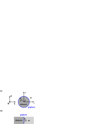
Figure 1: (a) Cross-sectional view of the spherical shell-shaped superscatterer at $y=0$ plane, where the dielectric particle (dark grey area) to be superscattered is coated with the graphene monolayer (blue area). A $x$-polarized plane wave is incident from air onto the superscatterer. (b) Structure of the equivalent planar waveguide, where the graphene monolayer (blue area) is separated by a semi-infinite dielectric medium (dark gray area) and the air (light gray area). The graphene plasmons propagate along the graphene surface in the direction indicated by an arrow.

Analytical Mie scattering theory is applied to solve this scattering problem bookEWPRS ; bookASLSP . Different from the 2D case where TM and TE waves are defined according to the axis of the cylinder OL40-1651 , the electromagnetic fields in 3D case can be decomposed into TM and TE waves with respect to the radial direction $\hat{r}$, namely $\mathbf{H}_{\text{TM}}=\nabla\times\left(\Phi_{\text{TM}}\mathbf{r}\right)$ and $\mathbf{E}_{\text{TE}}=\nabla\times\left(\Phi_{\text{TE}}\mathbf{r}\right)$, where $\Phi_{\text{TM}}$ is the electric potential and $\Phi_{\text{TE}}$ is the magnetic potential. For the incident field, its corresponding electric potential $\Phi_{\text{TM}}$ and magnetic potential $\Phi_{\text{TE}}$ are

$$\Phi_{\text{TM}}^{i}=-\frac{E_{0}\cos\phi}{k_{0}\eta_{0}r}\sum_{n=1}^{\infty}a_{n}\psi_{n}\left(k_{0}r\right)P_{n}^{1}\left(\cos\theta\right)$$ (1)

and

$$\Phi_{\text{TE}}^{i}=\frac{E_{0}\sin\phi}{k_{0}r}\sum_{n=1}^{\infty}a_{n}\psi_{n}\left(k_{0}r\right)P_{n}^{1}\left(\cos\theta\right)\,,$$ (2)

respectively, where $a_{n}=\left(-i\right)^{-n}\left(2n+1\right)/n\left(n+1\right)$ is the expansion coefficient. Similarly, scalar potentials are

$$\Phi_{\text{TM}}^{s}=-\frac{E_{0}\cos\phi}{k_{0}\eta_{0}r}\sum_{n=1}^{\infty}a_{n}s_{n}^{\text{TM}}\xi_{n}\left(k_{0}r\right)P_{n}^{1}\left(\cos\theta\right)$$ (3)

and

$$\Phi_{\text{TE}}^{s}=\frac{E_{0}\sin\phi}{k_{0}r}\sum_{n=1}^{\infty}a_{n}s_{n}^{\text{TE}}\xi_{n}\left(k_{0}r\right)P_{n}^{1}\left(\cos\theta\right)$$ (4)

for the scattered electromagnetic field at $r>R$, and

$$\Phi_{\text{TM}}^{in}=-\frac{E_{0}\cos\phi}{k\eta r}\sum_{n=1}^{\infty}a_{n}b_{n}^{\text{TM}}\psi_{n}\left(kr\right)P_{n}^{1}\left(\cos\theta\right)$$ (5)

and

$$\Phi_{\text{TE}}^{in}=\frac{E_{0}\sin\phi}{kr}\sum_{n=1}^{\infty}a_{n}b_{n}^{\text{TE}}\psi_{n}\left(kr\right)P_{n}^{1}\left(\cos\theta\right)$$ (6)

for the electromagnetic field inside the dielectric particle ($r\leq R$), where $k=k_{0}\sqrt{\varepsilon_{r}\mu_{r}}$ is the wavenumber in the dielectric particle, $s_{n}^{\text{TM}}$, $s_{n}^{\text{TE}}$, $b_{n}^{\text{TM}}$, and $b_{n}^{\text{TE}}$ are unknown expansion coefficients, $\psi_{n}\left(k_{0}r\right)$ and $\xi_{n}\left(k_{0}r\right)$ are the $n$-th order Riccati–Bessel function of the first kind and the third kind, respectively bookHMFFGMT . Meanwhile, $\eta=\sqrt{\mu_{0}\mu_{r}/\varepsilon_{0}\varepsilon_{r}}$ and $\eta_{0}=\sqrt{\mu_{0}/\varepsilon_{0}}$ are the impedances of the dielectric particle and free space, respectively. Since the thickness of graphene is extremely small compared with the radius of the spherical dielectric particle, the graphene coating can be well characterized as a two dimensional homogenized conducting film with surface conductivity $\sigma_{g}$, where the non-spherical elements and microscopic details are neglected science332-1291 ; JAP103-064302 ; PRB91-125414 . According to the continuity conditions at $r=R$, the scattering coefficient can be obtained as

$$s_{n}^{\text{TM}}=\frac{-\psi_{n}^{\prime}\left(k_{0}R\right)t_{n}^{\text{TM}}+\left(\eta/\eta_{0}\right)\psi_{n}\left(k_{0}R\right)\psi_{n}^{\prime}\left(kR\right)}{\xi_{n}^{\prime}\left(k_{0}R\right)t_{n}^{\text{TM}}-\left(\eta/\eta_{0}\right)\xi_{n}\left(k_{0}R\right)\psi_{n}^{\prime}\left(kR\right)}\,,$$ (7)

$$s_{n}^{\text{TE}}=\frac{-\psi_{n}\left(k_{0}R\right)t_{n}^{\text{TE}}+\left(\eta/\eta_{0}\right)\psi_{n}^{\prime}\left(k_{0}R\right)\psi_{n}\left(kR\right)}{\xi_{n}\left(k_{0}R\right)t_{n}^{\text{TE}}-\left(\eta/\eta_{0}\right)\xi_{n}^{\prime}\left(k_{0}R\right)\psi_{n}\left(kR\right)}\,,$$ (8)

where $t_{n}^{\text{TM}}=\psi_{n}\left(kR\right)+i\sigma_{g}\eta\psi_{n}^{\prime}\left(kR\right)$, $t_{n}^{\text{TE}}=\psi_{n}^{\prime}\left(kR\right)-i\sigma_{g}\eta\psi_{n}\left(kR\right)$, and $\sigma_{g}$ is the surface conductivity of graphene. We define the normalized scattering cross section (NSCS) as

$$\mathrm{NSCS}=\sum\limits_{n=1}^{\infty}\left(2n+1\right)\left(\left|s_{n}^{\text{TM}}\right|^{2}+\left|s_{n}^{\text{TE}}\right|^{2}\right)\,,$$ (9)

which is normalized by $\lambda^{2}/2\pi$. Note that when $\sigma_{g}=0$, it reduces to the case of scattering by a bare spherical dielectric particle.

The aforementioned scattering model is related to its equivalent one dimensional planar waveguide by Bohr model, where the structure of the planar waveguide is shown in Fig. 1 (b). To support a resonance, Bohr condition requires that the phase accumulation along an enclosed optical path should be an integral number of $2\pi$, namely

$$\oint\beta dl=2n\pi\,,$$ (10)

where $n$ is the order of the resonance, $\beta$ is the corresponding propagation constant in the equivalent planar waveguide, and the integral is calculated along the circumference of the sphere since graphene plasmons propagate as a surface wave along the graphene surface with evanescent fields in the perpendicular direction.

Meanwhile, in order to get the NSCS of the superscatterer shown in Fig. 1 (a) from Mie scattering theory and the propagation constant of the equivalent planar waveguide shown in Fig. 1 (b), the surface conductivity of graphene is calculated according to the Kubo formula

$$\sigma_{g}\left(\omega,\mu_{c},\Gamma,T\right)=\sigma_{\text{intra}}+\sigma_{\text{inter}}\,,$$ (11)

where

$$\sigma_{\text{intra}}=\frac{ie^{2}k_{B}T}{\pi\hbar^{2}\left(\omega+i2\Gamma\right)}\left[\frac{\mu_{c}}{k_{B}T}+2\ln\left(e^{-\mu_{c}/k_{B}T}+1\right)\right]$$ (12)

is due to intraband contribution, and

$$\sigma_{\text{inter}}=\frac{ie^{2}\left(\omega+i2\Gamma\right)}{\pi\hbar^{2}}\int_{0}^{\infty}\frac{f_{d}\left(-\varepsilon\right)-f_{d}\left(\varepsilon\right)}{\left(\omega+i2\Gamma\right)^{2}-4\left(\varepsilon/\hbar\right)^{2}}d\varepsilon$$ (13)

is due to interband contribution JAP103-064302 ; JP19-026222 . In the above formula, $-e$ is the charge of an electron, $\hbar=h/2\pi$ is the reduced Plank’s constant, $\Gamma$ is the phenomenological scattering rate that is assumed to be independent of the energy $\varepsilon$, $f_{d}\left(\varepsilon\right)=1/\left[e^{\left(\varepsilon-\mu_{c}\right)/k_{B}T}+1\right]$ is the Fermi-Dirac distribution, $k_{B}$ is the Boltzmann’s constant, $T$ is the temperature, and $\mu_{c}$ is the chemical potential which can be tuned by a gate voltage and/or chemical doping. In the following, we choose $\Gamma=0.11$ meV and $T=300$ K JAP103-064302 .

III Results and discussion

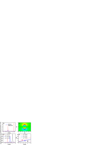
Figure 2: (a) The dependence of the normalized scattering cross section (NSCS) on the incident frequency $f$, where the graphene monolayer with $\mu_{c}=0.3$ eV is considered to be lossless or lossy. (b) Normalized $H_{\theta}$ field distribution at $z=0$ plane with $f=4.7$ THz when the optical loss of graphene is involved. (c) NSCSs for different frequencies when $\mu_{c}=0.2$ eV, $0.3$ eV, and $0.4$ eV, respectively. (d) Dispersion relations of TM graphene plasmons in the equivalent planar waveguide for $\mu_{c}=0.2$ eV, $0.3$ eV, and $0.4$ eV, respectively. The dotted magenta curve denotes the Bohr condition for superscattering, and three stars in the curve correspond to the three resonate frequencies in (c). The other parameters are $\varepsilon_{r}=1.44$ and $R=0.24$ $\mu$m.

To demonstrate the superscattering phenomenon for subwavelength particles, we let $\varepsilon_{r}=1.44$, $R=0.24$ $\mu$m, and $\mu_{c}=0.3$ eV JAP103-064302 . Under these parameters, Fig. 2 (a) schematically shows the dependence of the NSCS on the incident frequency $f$, where the graphene monolayer is considered to be lossless or lossy. When the optical loss of graphene is neglected with $\Gamma=0$ meV, two sharp resonances occur at $f=\omega/2\pi=4.7$ THz and $f=8.5$ THz, respectively. The corresponding NSCSs are close to their single channel limits $2n+1$ PRL105-013901 ; PRL97-263902 , where the resonances at $f=4.7$ THz and $f=8.5$ THz are dominated by the $n=1$ and $n=2$ scattering terms, respectively. When the optical loss is involved with $\Gamma\neq 0$ meV nnano6-630 ; SSC ; nphoton7-394 , the NSCSs at both two resonances decrease from their corresponding single channel limits due to the damping effects of graphene plasmons. As shown in Fig. 2 (a), the NSCS at the first order resonance ($n=1$) decreases to 0.62, while the NSCS at the second order resonance ($n=2$) decreases more sharply and is equal to zero approximately. This is because the second order resonance is more susceptible to the loss PRL105-013901 . As shown in Fig. 2 (b), the normalized $H_{\theta}$ field distribution exhibits a first order resonant mode at $f=4.7$ THz. Since the chemical potential of graphene can be tuned by a gate voltage and/or chemical doping JAP103-064302 , Fig. 2 (c) shows NSCSs for different frequencies at different values of chemical potential, where the decrease of peak NSCS at lower resonate frequencies is caused by the increasing optical loss of graphene JAP103-064302 . The NSCS of the bare dielectric particle is in the order of $10^{-6}$, this indicates that coating with a properly doped and/or gated graphene monolayer can greatly enhance the scattering by five orders of magnitude at certain frequencies. Meanwhile, larger chemical potential leads to superscattering at higher frequency, which can be understood with Bohr model.

In the above frequency range, the surface conductivity of graphene has a positive imaginary part, which implies that TM graphene plasmons are supported with the components $H_{\theta}$, $E_{\phi}$, and $E_{r}$ science332-1291 ; JAP103-064302 . For the spherical shell-shaped superscatterer, the dispersion relation of TM graphene plasmons in the equivalent planar waveguide is

$$\frac{\varepsilon_{r}}{k_{1}}+\frac{1}{k_{2}}+i\frac{\sigma_{g}}{\omega\varepsilon_{0}}=0,$$ (14)

where $k_{1}=\left(\beta^{2}-k_{0}^{2}\varepsilon_{r}\right)^{1/2}$, $k_{2}=\left(\beta^{2}-k_{0}^{2}\right)^{1/2}$, and $\beta$ is the propagation constant. Meanwhile, we define $\delta_{d}=1/k_{1}$ and $\delta_{a}=1/k_{2}$ as the penetration depths in the dielectric medium and air, respectively. Fig. 2 (d) shows the dispersion relations for $\mu_{c}=0.2$ eV, $0.3$ eV, and $0.4$ eV, where the optical loss of graphene is neglected. The first order Bohr condition $\beta=1/R$ for superscattering is denoted by the dotted magenta curve. According to the Bohr model, superscattering occurs at the intersection points of dispersion relations and the Bohr condition, which exhibits blue shift when the chemical potential of graphene increases. For comparison, resonant frequencies for $\mu_{c}=0.2$ eV, $0.3$ eV, and $0.4$ eV are calculated from Mie scattering theory and marked by three stars in the dotted magenta curve. Clearly, the stars exhibit blue shift similarly.

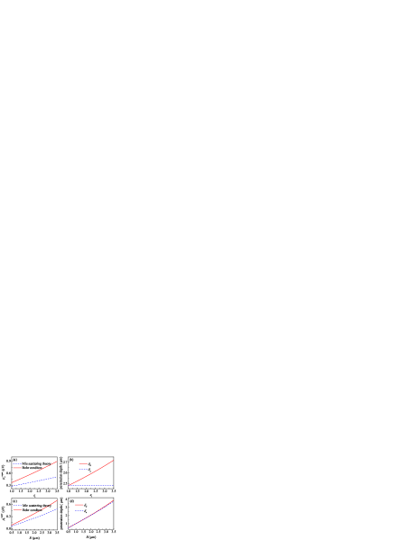
Figure 3: Left panel: The dependences of $\mu_{c}^{\text{super}}$ on the (a) relative permittivity $\varepsilon_{r}$ and (c) radius $R$, respectively, where superscattering occurs when $\mu_{c}=\mu_{c}^{\text{super}}$ under the corresponding value of $\varepsilon_{r}$ or $R$. The solid red curve and the dashed blue curve are calculated by Bohr condition and Mie scattering theory, respectively. Right panel: The dependences of the penetration depth ($\delta_{d}$ for the dielectric medium and $\delta_{a}$ for the air) on the (b) relative permittivity $\varepsilon_{r}$ and (d) radius $R$, respectively. The parameters are $R=0.24$ $\mu$m for (a) and (b), $\varepsilon_{r}=1.44$ for (c) and (d), and $f=5$ THz for (a)-(d).

As shown in Fig. 2 (d), star deviates from the intersection point at higher frequencies. In order to interpret this deviation, we first analyse a simple case. Fig. 3 (a) shows the dependence of the chemical potential $\mu_{c}^{\text{super}}$ on the relative permittivity of dielectric particle, where $\mu_{c}^{\text{super}}$ is the value of chemical potential when superscattering occurs. Once the radius of the sphere is fixed, the propagation constant $\beta$ is determined by the Bohr condition. However, the increase of the relative permittivity $\varepsilon_{r}$ leads to the increase of propagation constant $\beta$, which further leads to the increase of the chemical potential to ensure the invariance of the propagation constant. Moreover, since the penetration depth of graphene plasmons in the dielectric medium $\delta_{d}$ becomes large when $\varepsilon_{r}$ increases as shown in Fig. 3 (b), the calculation of the path integral along the circumference of the sphere is not accurate any more arxiv . This produces errors to the calculation of propagation constant $\beta$ and chemical potential $\mu_{c}$. Actually, the growth rate of chemical potential slows down to match a shorter integration path.

Although the radius of the sphere $R$ is not related directly to the penetration depths of graphene plasmons, a small value of propagation constant $\beta$ is required to support the resonance in a large sphere. This leads to the increase of chemical potential $\mu_{c}^{\text{super}}$ and penetration depths $\delta_{d}$ and $\delta_{a}$, which can be seen clearly from Fig. 3 (c)-(d). Since the penetration depth in the dielectric medium is larger than that in the air, the growth rate of chemical potential slows down to match a shorter integration path. Then we can use the same method to interpret the deviation in Fig. 2 (d). The increase of incident frequency is equivalent to an increase of the radius, thus deviation between Mie scattering theory and Bohr condition becomes large at high frequencies.

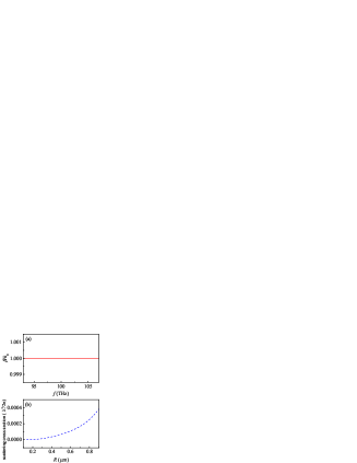
Figure 4: (a) Dispersion relation of TE graphene plasmons. (b) The dependence of the normalized scattering cross section (NSCS) on the radius $R$ with $f=100$ THz. The parameters are $\mu_{c}=0.2$ eV and $\varepsilon_{r}=1$.

From above analysis, we know that Bohr model provides an intuitive way to understand the superscattering of subwavelength particles and to design corresponding 3D superscatterers. For example, based on the Bohr model, we can predict the nonexistence of superscattering via the resonance of TE graphene plasmons. We let $f=100$ THz, $\varepsilon_{r}=1$, and $\mu_{c}=0.2$ eV, since TE graphene plasmons do not exist for $\varepsilon_{r}=1.44$. Under these parameters, the surface conductivity of graphene has a negative imaginary part, which implies that the TE graphene plasmons are supported with the components $E_{\theta}$, $H_{\phi}$, and $H_{r}$ science332-1291 ; JAP103-064302 . The dispersion relation of TE graphene plasmons in the equivalent planar waveguide is

$$k_{1}+k_{2}-i\sigma_{g}\omega\mu_{0}=0,$$ (15)

where $k_{1}$, $k_{2}$, and $\beta$ are the same as in Eq. (14). According to Bohr condition, superscattering should occur at $R=1/k_{0}=3/2\pi$ $\mu$m, where we have replaced the propagation constant of TE graphene plasmons by the wave number in air since $\beta\approx k_{0}$ as shown in Fig. 4 (a). However, no superscattering occurs as shown in Fig. 4 (b). The reason is that no appropriate integration path can be used to match the Bohr condition due to poor field confinements of TE graphene plasmons.

IV Conclusions

In conclusion, we demonstrate for the first time that graphene monolayers can be used for atomically thin spherical shell-shaped superscatterer designs. The first-order resonance of TM graphene plasmons can be excited to enhance the scattering cross section of the bare subwavelength dielectric particle by five orders of magnitude. Scientifically, Bohr model is used to understand and interpret the superscattering phenomenon. Based on the analysis of Bohr model, we show that contrary to the TM case, superscattering is hard to occur by exciting the resonance of TE graphene plasmons due to their poor field confinements. Our work will provide theoretical guidance for the future experimental design of superscatterers and other graphene based devices, which have great potential applications in sub-wavelength plasmonics.

References

- (1) N. Zheludev and Y. Kivshar, Nat. Mater., 2012, 11, 917-924.
- (2) A. E. Minovich, A. E. Miroshnichenko, A. Y. Bykov, T. V. Murzina, D. N. Neshev, and Y. S. Kivshar, Laser Photon. Rev., 2015, 9, 195-213.
- (3) M. S. Kushwaha, and B. Djafari-Rouhani, J. Opt. Soc. Am. B, 2010, 27, 148-167.
- (4) M. S. Kushwaha, and B. Djafari-Rouhani, Mod. Phys. Lett. B, 2013, 27, 1330013.
- (5) P.-Y. Chen, and A. Alù, ACS Nano, 2011, 5, 5855-5863.
- (6) M. Farhat, C. Rockstuhl, and H. Bağcı, Opt. Exp., 2013, 21, 12592-12603.
- (7) H. M. Bernety, and A. B. Yakovlev, J. Phys.: Condens. Matter, 2015, 27, 185304.
- (8) T. Yang, H. Chen, X. Luo, and H. Ma, Opt. Exp., 2008, 16, 18545-18550.
- (9) S. Nie and S. R. Emory, Science, 1997, 275, 1102-1106.
- (10) J. B. Jackson and N. J. Halas, Proc. Natl. Acad. Sci. U.S.A., 2004, 101, 17930-17935.
- (11) R. Bardhan, S. Mukherjee, N. A. Mirin, S. D. Levit, P. Nordlander, and N. J. Halas, J. Phys. Chem. C, 2010, 114, 7378-7383.
- (12) H. R. Stuart and D. G. Hall, Appl. Phys. Lett., 1998, 73, 3815-3817.
- (13) F. Hao, Y. Sonnefraud, P. V. Dorpe, S. A. Maier, N. J. Halas, and P. Nordlander, Nano Lett., 2008, 8, 3983-3988.
- (14) J. Aizpurua, P. Hanarp, D. S. Sutherland, M. Käll, G. W. Bryant, and F. J. Garcia de Abajo, Phys. Rev. Lett., 2003, 90, 057401.
- (15) S. Pillai, K. R. Catchpole, T. Trupke, and M. A. Green, J. Appl. Phys., 2007, 101, 093105.
- (16) H. A. Atwater and A. Polman, Nat. Mater., 2010, 9, 205-213.
- (17) H. Chen, X. Zhang, X. Luo, H. Ma, and C. T. Chan, New J. Phys., 2008, 10, 113016.
- (18) X. Luo, T. Yang, Y. Gu, H. Chen, and H. Ma, Appl. Phys. Lett., 2009, 94, 223513.
- (19) W. H. Wee and J. B. Pendry, New J. Phys., 2009, 11, 073033.
- (20) X. Zang, and C. Jiang, Opt. Exp., 2010, 18, 6891-6899.
- (21) C. Yang, J. Yang, M. Huang, J. Peng , G. Cai, Comp. Mater. Sci., 2010, 49, 820-825.
- (22) W. Jiang, B. Xu, Q. Cheng, T. Cui, and G. Yu, J. Opt. Soc. Am. A, 2013, 30, 1698-1702.
- (23) Z. Ruan and S. Fan, Phys. Rev. Lett., 2010, 105, 013901.
- (24) Z. Ruan and S. Fan, Appl. Phys. Lett., 2011, 98, 043101.
- (25) L. Verslegers, Z. Yu, Z. Ruan, P. B. Catrysse, and S. Fan, Phys. Rev. Lett., 2012, 108, 083902.
- (26) H. L. Chen and L. Gao, Phys. Rev. A, 2012, 86, 033825.
- (27) A. Mirzaei, I. V. Shadrivov, A. E. Miroshnichenko, and Y. S. Kivshar, Opt. Exp., 2013, 21, 10454-10459.
- (28) A. Mirzaei, A. E. Miroshnichenko, I. V. Shadrivov, and Y. S. Kivshar, Appl. Phys. Lett., 2014, 105, 011109.
- (29) Y. Huang and L. Gao, J. Phys. Chem. C, 2014, 118, 30170-30178.
- (30) W. Wan, W. Zheng, Y. Chen, and Z. Liu, Nanoscale, 2014, 6, 9093-9102.
- (31) T. Yang, R. Cao, X. Luo, and H. Ma, Appl. Phys. A, 2010, 99, 843-847.
- (32) L. Zhao, B. Liu, Y. Gao, Y. Zhao, and J. Huang, Front. Phys., 2012, 7, 323.
- (33) R. Li, X. Lin, S. Lin, X. Liu, and H. Chen, Opt. Lett., 2015, 40, 1651-1654.
- (34) A. H. Castro Neto, F. Guinea, N. M. R. Peres, K. S. Novoselov, and A. K. Geim, Rev. Modern Phys., 2009, 81, 109-162.
- (35) A. Vakil and N. Engheta, Science, 2011, 332, 1291-1294.
- (36) D. Dragoman and M. Dragomann, Quantum-Classical Analogies (Springer, Berlin, 2004).
- (37) S. Longhi, Laser Photon. Rev., 2009, 3, 243-261.
- (38) K. G. Makris, R. El-Ganainy, and D. N. Christodoulides, Phys. Rev. Lett., 2008, 100, 103904.
- (39) C. E. Rüter, K. G. Makris, R. El-Ganainy, D. N. Christodoulides, M. Segev, and D. Kip, Nat. Phys., 2010, 6, 192-195.
- (40) A. Guo, G. J. Salamo, D. Duchesne, R. Morandotti, M. Volatier-Ravat, V. Aimez, G. A. Siviloglou, and D. N. Christodoulides, Phys. Rev. Lett., 2009, 103, 093902.
- (41) M.-A. Miri, M. Heinrich, R. El-Ganainy, and D. N. Christodoulides, Phys. Rev. Lett., 2013, 110, 233902.
- (42) M.-A. Miri, M. Heinrich, and D. N. Christodoulides, Optica, 2014, 1, 89-95.
- (43) M. Segev, Y. Silberberg, and D. N. Christodoulides, Nat. Photon., 2013, 7, 197-204.
- (44) K. Manouchehri, J. Wang, Physical Implementation of Quantum Walks (Springer, Berlin, 2014).
- (45) S. G. Krivoshlykov, Quantum-Theoretical Formalism for Inhomogeneous Graded-Index Waveguides (Akademie Verlag, Berlin, 1994).
- (46) J. D. Joannopoulos, S. G. Johnson, J. N. Winn, R. D. Meade, Photonic Crystals: Molding the Flow of Light, 2nd ed. (Princeton University Press, New Jersey, 2008).
- (47) I. L. Garanovich, S. Longhi, A. A. Sukhorukova, Y. S. Kivshar, Phys. Rep., 2012, 518, 1-79.
- (48) W. Liu, R. F. Oulton, and Y. S. Kivshar, Sci. Rep., 2015, 5, 12148.
- (49) X. Lia, W. Chen, S. Zhang, Z. Wu, P. Wang, Z. Xua, H. Chen, W. Yin, H. Zhong, S. Lin, Nano Energy, 2015, 16, 310-319.
- (50) S. Lin, B. Chen, W. Xiong, Y. Yang, H. He, and J. Luo, Opt. Exp., 2012, 20, A706-A712.
- (51) A. Ishimaru, Electromagnetic Wave Propagation, Radiation, and Scattering (Prentice-Hall, New Jersey, 1991).
- (52) C. F. Bohren and D. R. Huffman, Absorption and Scattering of Light by Small Particles (Wiley, New York, 1983).
- (53) M. Abramowitz and I. A. Stegun, Handbook of Mathematical Functions with Formulas, Graphs, and Mathematical Tables (Dover, New York, 1965).
- (54) G. W. Hanson, J. Appl. Phys., 2008, 103, 064302.
- (55) T. Christensen, A.-P. Jauho, M. Wubs, and N. A. Mortensen, Phys. Rev. B, 2015, 91, 125414.
- (56) V. P. Gusynin, S. G. Sharapov, and J. P. Carbotte, J. Phys.: Condens. Matter, 2007, 19, 026222.
- (57) M. I. Tribelsky and B. S. Luk’yanchuk, Phys. Rev. Lett., 2006, 97, 263902.
- (58) L. Ju, B. Geng, J. Horng, C. Girit, M. Martin, Z. Hao, H. A. Bechtel, X. Liang, A. Zettl, Y. R. Shen, and F. Wang, Nat. Nanotechnol., 2011, 6, 630 C634.
- (59) K. I. Bolotin, K. J. Sikes, Z. Jianga, M. Klima, G. Fudenberg, J. Hone, P. Kim, and H. L. Stormer, Solid State Commun., 2008, 146, 351-355.
- (60) H. Yan, T. Low, W. Zhu, Y. Wu, M. Freitag, X. Li, F. Guinea, P. Avouris, and F. Xia, Nat. Photon., 2013, 7, 394-399.