1 Main results
We consider the charged planar three-body problem concerns of 3 point particles endowed with a positive
mass m j ∈ 𝐑 + = { r ∈ 𝐑 | r > 0 } subscript 𝑚 𝑗 superscript 𝐑 conditional-set 𝑟 𝐑 𝑟 0 m_{j}\in{\bf R}^{+}=\{r\in{\bf R}\;|\;r>0\} e j ∈ 𝐑 , j = 1 , 2 , 3 formulae-sequence subscript 𝑒 𝑗 𝐑 𝑗 1 2 3
e_{j}\in{\bf R},j=1,2,3 q 1 , q 2 , q 3 ∈ 𝐑 2 subscript 𝑞 1 subscript 𝑞 2 subscript 𝑞 3
superscript 𝐑 2 q_{1},q_{2},q_{3}\in{\bf R}^{2}
m i q ¨ i = ∑ j ≠ i m i m j − e i e j | q i − q j | 3 ( q j − q i ) = ∂ U ( q ) ∂ q i , for i = 1 , 2 , 3 , formulae-sequence subscript 𝑚 𝑖 subscript ¨ 𝑞 𝑖 subscript 𝑗 𝑖 subscript 𝑚 𝑖 subscript 𝑚 𝑗 subscript 𝑒 𝑖 subscript 𝑒 𝑗 superscript subscript 𝑞 𝑖 subscript 𝑞 𝑗 3 subscript 𝑞 𝑗 subscript 𝑞 𝑖 𝑈 𝑞 subscript 𝑞 𝑖 for 𝑖
1 2 3
m_{i}\ddot{q}_{i}=\sum_{j\neq i}\frac{m_{i}m_{j}-e_{i}e_{j}}{|q_{i}-q_{j}|^{3}}(q_{j}-q_{i})=\frac{\partial U(q)}{\partial q_{i}},\qquad{\rm for}\quad i=1,2,3, (1.1)
where U ( q ) = U ( q 1 , q 2 , q 3 ) = ∑ 1 ≤ i < j ≤ 3 m i m j − e i e j | q i − q j | 𝑈 𝑞 𝑈 subscript 𝑞 1 subscript 𝑞 2 subscript 𝑞 3 subscript 1 𝑖 𝑗 3 subscript 𝑚 𝑖 subscript 𝑚 𝑗 subscript 𝑒 𝑖 subscript 𝑒 𝑗 subscript 𝑞 𝑖 subscript 𝑞 𝑗 U(q)=U(q_{1},q_{2},q_{3})=\sum_{1\leq i<j\leq 3}\frac{m_{i}m_{j}-e_{i}e_{j}}{|q_{i}-q_{j}|} | ⋅ | |\cdot| 𝐑 2 superscript 𝐑 2 {\bf R}^{2} 2 π 2 𝜋 2\pi 1.1
𝒜 ( q ) = ∫ 0 2 π [ ∑ i = 1 3 m i | q ˙ i ( t ) | 2 2 + U ( q ( t ) ) ] 𝑑 t 𝒜 𝑞 superscript subscript 0 2 𝜋 delimited-[] superscript subscript 𝑖 1 3 subscript 𝑚 𝑖 superscript subscript ˙ 𝑞 𝑖 𝑡 2 2 𝑈 𝑞 𝑡 differential-d 𝑡 \mathcal{A}(q)=\int_{0}^{2\pi}\left[\sum_{i=1}^{3}\frac{m_{i}|\dot{q}_{i}(t)|^{2}}{2}+U(q(t))\right]dt
defined on the loop space W 1 , 2 ( 𝐑 / ( 2 π 𝐙 ) , 𝒳 ^ ) superscript 𝑊 1 2
𝐑 2 𝜋 𝐙 ^ 𝒳 W^{1,2}({\bf R}/(2\pi{\bf Z}),\hat{\mathcal{X}})
𝒳 ^ = { q = ( q 1 , q 2 , q 3 ) ∈ ( 𝐑 2 ) 3 | ∑ i = 1 3 m i q i = 0 , q i ≠ q j , ∀ i ≠ j } ^ 𝒳 conditional-set 𝑞 subscript 𝑞 1 subscript 𝑞 2 subscript 𝑞 3 superscript superscript 𝐑 2 3 formulae-sequence superscript subscript 𝑖 1 3 subscript 𝑚 𝑖 subscript 𝑞 𝑖 0 formulae-sequence subscript 𝑞 𝑖 subscript 𝑞 𝑗 for-all 𝑖 𝑗 \hat{\mathcal{X}}=\left\{q=(q_{1},q_{2},q_{3})\in({\bf R}^{2})^{3}\,\,\left|\,\,\sum_{i=1}^{3}m_{i}q_{i}=0,\,\,q_{i}\neq q_{j},\,\,\forall i\neq j\right.\right\}
is the configuration space of the planar three-body problem. Periodic solutions of (1.1 𝒜 𝒜 \mathcal{A}
It is a well-known fact that (1.1 p 1 , p 2 , p 3 ∈ 𝐑 2 subscript 𝑝 1 subscript 𝑝 2 subscript 𝑝 3
superscript 𝐑 2 p_{1},p_{2},p_{3}\in{\bf R}^{2} 1.1
p ˙ i = − ∂ H ∂ q i , q ˙ i = ∂ H ∂ p i , for i = 1 , 2 , 3 , formulae-sequence subscript ˙ 𝑝 𝑖 𝐻 subscript 𝑞 𝑖 formulae-sequence subscript ˙ 𝑞 𝑖 𝐻 subscript 𝑝 𝑖 for
𝑖 1 2 3
\dot{p}_{i}=-\frac{\partial H}{\partial q_{i}},\,\,\dot{q}_{i}=\frac{\partial H}{\partial p_{i}},\qquad{\rm for}\quad i=1,2,3, (1.2)
with Hamiltonian function
H ( p , q ) = H ( p 1 , p 2 , p 3 , q 1 , q 2 , q 3 ) = ∑ i = 1 3 | p i | 2 2 m i − U ( q 1 , q 2 , q 3 ) . 𝐻 𝑝 𝑞 𝐻 subscript 𝑝 1 subscript 𝑝 2 subscript 𝑝 3 subscript 𝑞 1 subscript 𝑞 2 subscript 𝑞 3 superscript subscript 𝑖 1 3 superscript subscript 𝑝 𝑖 2 2 subscript 𝑚 𝑖 𝑈 subscript 𝑞 1 subscript 𝑞 2 subscript 𝑞 3 H(p,q)=H(p_{1},p_{2},p_{3},q_{1},q_{2},q_{3})=\sum_{i=1}^{3}\frac{|p_{i}|^{2}}{2m_{i}}-U(q_{1},q_{2},q_{3}). (1.3)
Note that if all charges are zero, the problem reduces to the classical Newtonian one. The charged problem
has a more complicated dynamical behavior.
Central configurations are basic topics which help understanding the complexity of the
charged problem. It is well known that, in the classical Newtonian three-body problem, there are five central
configurations: two of them are equilateral triangles and three of them are collinear. In the charged problem,
Peréz-Chavela, Sarri, Susin and Yan ([17 ] , 1996) proved that there might exist at most five collinear central
configurations under some constraints of the parameters (masses and quantities of electric charge). They also
proved that, if there exist non-collinear central configurations, the shape of such central configuration is
determined by the masses and quantities of electric charge, and hence may not be an equilateral triangle in
general.
In the charged three-body problem, when the three bodies form a central configuration and each of which
move along a Keplerian orbit with eccentricity e ∈ [ 0 , 1 ) 𝑒 0 1 e\in[0,1) 1.1 elliptic relative equilibria . Specially when e = 0 𝑒 0 e=0 relative equilibria traditionally.
Our main concern in this paper is the linear stability of these homographic solutions.
For the planar three-body problem with masses m 1 , m 2 , m 3 > 0 subscript 𝑚 1 subscript 𝑚 2 subscript 𝑚 3
0 m_{1},m_{2},m_{3}>0 e 1 , e 2 , e 3 ∈ 𝐑 subscript 𝑒 1 subscript 𝑒 2 subscript 𝑒 3
𝐑 e_{1},e_{2},e_{3}\in{\bf R} e ∈ [ 0 , 1 ) 𝑒 0 1 e\in[0,1) β ∈ [ 0 , 9 ] 𝛽 0 9 \beta\in[0,9]
β = 36 ( m 1 m 2 sin 2 θ 3 + m 1 m 3 sin 2 θ 2 + m 2 m 3 sin 2 θ 1 ) ( m 1 + m 2 + m 3 ) 2 , 𝛽 36 subscript 𝑚 1 subscript 𝑚 2 superscript 2 subscript 𝜃 3 subscript 𝑚 1 subscript 𝑚 3 superscript 2 subscript 𝜃 2 subscript 𝑚 2 subscript 𝑚 3 superscript 2 subscript 𝜃 1 superscript subscript 𝑚 1 subscript 𝑚 2 subscript 𝑚 3 2 \beta=\frac{36(m_{1}m_{2}\sin^{2}\theta_{3}+m_{1}m_{3}\sin^{2}\theta_{2}+m_{2}m_{3}\sin^{2}\theta_{1})}{(m_{1}+m_{2}+m_{3})^{2}}, (1.4)
where θ i , i = 1 , 2 , 3 formulae-sequence subscript 𝜃 𝑖 𝑖
1 2 3
\theta_{i},i=1,2,3 θ i = π 3 subscript 𝜃 𝑖 𝜋 3 \theta_{i}=\frac{\pi}{3} i = 1 , 2 , 3 𝑖 1 2 3
i=1,2,3 β 𝛽 \beta 1.4 β 𝛽 \beta [6 ] in the Newtonian case.
In [17 ] of 1996 of Pérez-Chavela, Saari, Susin, and Yan, and [1 ] of 2008 of Alfaro and
Pérez-Chavela, the authors considered the relative equilibria and their stabilities of three charged bodies
moving under the influence of the respective Newtonian and Colombian forces. In Section 4 of [17 ] , the
authors proved that, in the charged three-body problem, if δ i j > 0 subscript 𝛿 𝑖 𝑗 0 \delta_{ij}>0 1 ≤ i < j ≤ 3 1 𝑖 𝑗 3 1\leq i<j\leq 3 2.3 δ 12 1 / 3 superscript subscript 𝛿 12 1 3 \delta_{12}^{1/3} δ 23 1 / 3 superscript subscript 𝛿 23 1 3 \delta_{23}^{1/3} δ 31 1 / 3 superscript subscript 𝛿 31 1 3 \delta_{31}^{1/3} [1 ] (cf. p. 1940), the authors proved that, a non-collinear relative
equilibrium of charged three-body problem is both linearly stable and non-degenerate if and only if the masses and
charges satisfy the condition β < 1 𝛽 1 \beta<1 e = 0 𝑒 0 e=0
The linear stability of relative equilibria in the Newtonian case were known more than a century ago and it is due
to Gascheau ([4 ] , 1843) and Routh ([19 ] , 1875) independently. Further studies can be found in works of
Danby ([3 ] , 1964) and Roberts ([18 ] , 2002). In 2005, Meyer and Schmidt (cf. [16 ] )
used heavily the central configuration nature of the elliptic Lagrangian orbits and decomposed the fundamental
solution of the elliptic Lagrangian solution into two parts symplectically, one of which is the same as that of the
Keplerian solution and the other is the essential part for the stability.
Here we point out first that a flat homographic solution must be planar in the charged case. The proof in
[12 ] (cf. pp. 39-41) and [11 ] (cf. Theorem 2.6) for the Newtonian case works also for our problem with
some minor modifications when δ i j ≠ 0 subscript 𝛿 𝑖 𝑗 0 \delta_{ij}\neq 0 1 ≤ i < j ≤ 3 1 𝑖 𝑗 3 1\leq i<j\leq 3 [1 ] in the charged n 𝑛 n δ i j subscript 𝛿 𝑖 𝑗 \delta_{ij}
In this paper, following the central configuration coordinate method of Meyer and Schmidt in [16 ] ,
we linearize the Hamiltonian system (1.2 1.3 [9 ] ), i.e., the system (17) on p.275 of [16 ] (cf. also (2.19) in [6 ] ) depending
on the eccentricity e ∈ [ 0 , 1 ) 𝑒 0 1 e\in[0,1) β ∈ [ 0 , 9 ] 𝛽 0 9 \beta\in[0,9] 1.4 θ i = π / 3 subscript 𝜃 𝑖 𝜋 3 {\theta}_{i}=\pi/3 i = 1 𝑖 1 i=1 2 2 2 3 3 3 β 𝛽 \beta 1.4 [ 0 , 9 ] 0 9 [0,9]
Theorem 1.1 Let q ( t ) = ( r ( t ) R ( θ ( t ) ) a 1 , r ( t ) R ( θ ( t ) ) a 2 , r ( t ) R ( θ ( t ) ) a 3 ) 𝑞 𝑡 𝑟 𝑡 𝑅 𝜃 𝑡 subscript 𝑎 1 𝑟 𝑡 𝑅 𝜃 𝑡 subscript 𝑎 2 𝑟 𝑡 𝑅 𝜃 𝑡 subscript 𝑎 3 q(t)=(r(t)R(\theta(t))a_{1},r(t)R(\theta(t))a_{2},r(t)R(\theta(t))a_{3}) 1.1 δ i j > 0 subscript 𝛿 𝑖 𝑗 0 \delta_{ij}>0 1 ≤ i < j ≤ 3 1 𝑖 𝑗 3 1\leq i<j\leq 3 ( a 1 , a 2 , a 3 ) subscript 𝑎 1 subscript 𝑎 2 subscript 𝑎 3 (a_{1},a_{2},a_{3}) 1.1 q 𝑞 q e ∈ [ 0 , 1 ) 𝑒 0 1 e\in[0,1) β ∈ [ 0 , 9 ] 𝛽 0 9 \beta\in[0,9] 1.4
In 2004-2006, Martínez, Samà and Simó ([13 ] ,[14 ] ,[15 ] , 2004-2006) studied the
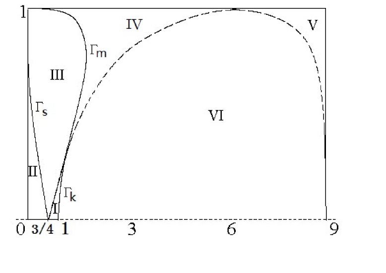
stability of the elliptic Lagrangian solution of the classical three body problem when e > 0 𝑒 0 e>0 e < 1 𝑒 1 e<1 1 1 1 [15 ] ) was drawn there for the full ( β , e ) 𝛽 𝑒 ({\beta},e)
Figure 1: Stability bifurcation diagram of elliptic relative equilibria of the charged and classical three-body problem
in the ( β , e ) 𝛽 𝑒 (\beta,e) [ 0 , 9 ] × [ 0 , 1 ) 0 9 0 1 [0,9]\times[0,1)
Denote the fundamental solution of the linearized Hamiltonian system of the essential part of the elliptic relative
equilibrium by γ β , e ( t ) subscript 𝛾 𝛽 𝑒
𝑡 {\gamma}_{{\beta},e}(t) t ∈ [ 0 , 2 π ] 𝑡 0 2 𝜋 t\in[0,2\pi] 𝐔 𝐔 {\bf U} 𝐂 𝐂 {\bf C} [15 ] , the following notations for the different parameter regions are used in Figure 1:
∙ ∙ \bullet
EE (elliptic-elliptic), if γ β , e ( 2 π ) subscript 𝛾 𝛽 𝑒
2 𝜋 {\gamma}_{{\beta},e}(2\pi) 𝐔 ∖ 𝐑 𝐔 𝐑 {\bf U}\setminus{\bf R}
∙ ∙ \bullet
EH (elliptic-hyperbolic), if γ β , e ( 2 π ) subscript 𝛾 𝛽 𝑒
2 𝜋 {\gamma}_{{\beta},e}(2\pi) 𝐔 ∖ 𝐑 𝐔 𝐑 {\bf U}\setminus{\bf R} 𝐑 ∖ { 0 , ± 1 } 𝐑 0 plus-or-minus 1 {\bf R}\setminus\{0,\pm 1\}
∙ ∙ \bullet
HH (hyperbolic-hyperbolic), if σ ( γ β , e ( 2 π ) ) ⊂ 𝐑 ∖ { 0 , ± 1 } 𝜎 subscript 𝛾 𝛽 𝑒
2 𝜋 𝐑 0 plus-or-minus 1 {\sigma}({\gamma}_{{\beta},e}(2\pi))\;\subset\;{\bf R}\setminus\{0,\pm 1\}
∙ ∙ \bullet
CS (complex-saddle), if σ ( γ β , e ( 2 π ) ) ⊂ 𝐂 ∖ ( 𝐔 ∪ 𝐑 ) 𝜎 subscript 𝛾 𝛽 𝑒
2 𝜋 𝐂 𝐔 𝐑 {\sigma}({\gamma}_{{\beta},e}(2\pi))\;\subset\;{\bf C}\setminus({\bf U}\cup{\bf R})
In [7 ] and [8 ] of 2009-2010, Hu and Sun found a new way to relate the stability problem to the
iterated Morse indices. Recently, by observing new phenomenons and discovering new properties of elliptic Lagrangian
solution, in the joint paper [6 ] of Hu, Long and Sun, the linear stability of elliptic Lagrangian solution
is completely solved analytically by index theory (cf. [10 ] ) and the new results are related directly to
( β , e ) 𝛽 𝑒 (\beta,e) Θ = [ 0 , 9 ] × [ 0 , 1 ) Θ 0 9 0 1 \Theta=[0,9]\times[0,1)
Then by our Theorem 1.1 and Theorem 2.3 below, which yields the minimization property of these elliptic relative
equilibria and then the values of the corresponding Morse indices of the corresponding functional at β = 0 𝛽 0 \beta=0 [6 ] as well as [15 ] can be applied to the linear stability problem of the elliptic
relative equilibria of the charged 3-body problem. Specially following [6 ] we have
Corollary 1.2 (i) The elliptic relative equilibrium q β , e subscript 𝑞 𝛽 𝑒
q_{{\beta},e} ( β , e ) ∈ [ 0 , 9 ] × [ 0 , 1 ) 𝛽 𝑒 0 9 0 1 ({\beta},e)\in[0,9]\times[0,1) i 1 ( q ) = 0 subscript 𝑖 1 𝑞 0 i_{1}(q)=0 γ β , e subscript 𝛾 𝛽 𝑒
{\gamma}_{{\beta},e} 1.1 q β , e subscript 𝑞 𝛽 𝑒
q_{{\beta},e} ν 1 ( γ β , e ) = 0 subscript 𝜈 1 subscript 𝛾 𝛽 𝑒
0 \nu_{1}({\gamma}_{{\beta},e})=0 β > 0 𝛽 0 \beta>0 ν 1 ( γ β , e ) = 3 subscript 𝜈 1 subscript 𝛾 𝛽 𝑒
3 \nu_{1}({\gamma}_{{\beta},e})=3 β = 0 𝛽 0 \beta=0
(ii) In the ( β , e ) 𝛽 𝑒 (\beta,e) Θ = ( 0 , 9 ] × [ 0 , 1 ) Θ 0 9 0 1 \Theta=(0,9]\times[0,1) Γ s subscript Γ 𝑠 \Gamma_{s} Γ m subscript Γ 𝑚 \Gamma_{m} ( 3 / 4 , 0 ) 3 4 0 (3/4,0) − 33 / 4 33 4 -\sqrt{33}/4 33 / 4 33 4 \sqrt{33}/4 ( 0 , 1 ) 0 1 (0,1) Γ k subscript Γ 𝑘 \Gamma_{k} ( 1 , 0 ) 1 0 (1,0) ( 0 , 1 ) 0 1 (0,1) e 𝑒 e e = 𝑐𝑜𝑛𝑠𝑡𝑎𝑛𝑡 ∈ [ 0 , 1 ) 𝑒 𝑐𝑜𝑛𝑠𝑡𝑎𝑛𝑡 0 1 e={\it constant}\;\in[0,1) ( β , e ) 𝛽 𝑒 (\beta,e) Γ s subscript Γ 𝑠 \Gamma_{s} Γ m subscript Γ 𝑚 \Gamma_{m} Γ k subscript Γ 𝑘 \Gamma_{k} Θ Θ \Theta Γ s subscript Γ 𝑠 \Gamma_{s} Γ s subscript Γ 𝑠 \Gamma_{s} Γ m subscript Γ 𝑚 \Gamma_{m} Γ m subscript Γ 𝑚 \Gamma_{m} Γ k subscript Γ 𝑘 \Gamma_{k} Γ k subscript Γ 𝑘 \Gamma_{k}
(iii) When e = 0 𝑒 0 e=0 q β , e subscript 𝑞 𝛽 𝑒
q_{{\beta},e} 0 < β < 1 0 𝛽 1 0<\beta<1 β = 1 𝛽 1 \beta=1 β > 1 𝛽 1 \beta>1
Proof. By our Theorems 1.1 and 2.3, the index properties of q β , e subscript 𝑞 𝛽 𝑒
q_{{\beta},e} β = 0 𝛽 0 {\beta}=0 [6 ] can be applied to get the corollary. Then (ii) and (iii)
follow from Theorems 1.2 and 1.5-1.8 of [6 ] .
Note first that more stability information for ( β , e ) 𝛽 𝑒 (\beta,e) [6 ] , and is omitted here. Note also that when e = 0 𝑒 0 e=0 q β , e subscript 𝑞 𝛽 𝑒
q_{{\beta},e} β > 0 𝛽 0 \beta>0 0 < β < 1 0 𝛽 1 0<\beta<1 [1 ] .
This paper is arranged as follows. In Section 2, we study elliptic relative equilibria of the charged three
body problem and their relations with the corresponding central configurations, and their variational
minimization property. Then in Section 3 we give the proof of Theorem 1.1.
2 Central configurations and minimizing property of the relative equilibria of the charged problem
We need the concept of central configurations in the charged problem as in [17 ] similar to the Newtonian case.
Definition 2.1 A configuration a = ( a 1 , a 2 , … , a n ) ∈ ( 𝐑 k ) n 𝑎 subscript 𝑎 1 subscript 𝑎 2 … subscript 𝑎 𝑛 superscript superscript 𝐑 𝑘 𝑛 a=(a_{1},a_{2},...,a_{n})\in({\bf R}^{k})^{n} a i ≠ a j , ∀ 1 ≤ i < j ≤ n formulae-sequence subscript 𝑎 𝑖 subscript 𝑎 𝑗 for-all 1 𝑖 𝑗 𝑛 a_{i}\neq a_{j},\forall 1\leq i<j\leq n m = ( m 1 , m 2 , … , m n ) ∈ ( 𝐑 + ) n 𝑚 subscript 𝑚 1 subscript 𝑚 2 … subscript 𝑚 𝑛 superscript superscript 𝐑 𝑛 m=(m_{1},m_{2},...,m_{n})\in({\bf R}^{+})^{n} e = ( e i , … , e j ) ∈ 𝐑 n 𝑒 subscript 𝑒 𝑖 … subscript 𝑒 𝑗 superscript 𝐑 𝑛 e=(e_{i},\ldots,e_{j})\in{\bf R}^{n} λ ∈ 𝐑 𝜆 𝐑 \lambda\in{\bf R} ( q , λ ) 𝑞 𝜆 (q,\lambda)
λ M a + ∂ U ( a ) ∂ q = 0 , 𝜆 𝑀 𝑎 𝑈 𝑎 𝑞 0 \lambda Ma+\frac{\partial U(a)}{\partial q}=0, (2.1)
with M = diag ( m 1 I k , … , m n I k ) 𝑀 diag subscript 𝑚 1 subscript 𝐼 𝑘 … subscript 𝑚 𝑛 subscript 𝐼 𝑘 M={\rm diag}(m_{1}I_{k},\ldots,m_{n}I_{k}) U 𝑈 U − 1 1 -1 2.1
λ = U ( a ) / ( M a ⋅ a ) . 𝜆 𝑈 𝑎 ⋅ 𝑀 𝑎 𝑎 \lambda=U(a)/(Ma\cdot a). (2.2)
In this paper, we only need the definition with k = 2 𝑘 2 k=2
δ i j = m i m j − e i e j m i m j = 1 − e i m i e j m j . subscript 𝛿 𝑖 𝑗 subscript 𝑚 𝑖 subscript 𝑚 𝑗 subscript 𝑒 𝑖 subscript 𝑒 𝑗 subscript 𝑚 𝑖 subscript 𝑚 𝑗 1 subscript 𝑒 𝑖 subscript 𝑚 𝑖 subscript 𝑒 𝑗 subscript 𝑚 𝑗 \delta_{ij}=\frac{m_{i}m_{j}-e_{i}e_{j}}{m_{i}m_{j}}=1-\frac{e_{i}}{m_{i}}\frac{e_{j}}{m_{j}}. (2.3)
Proposition 2.2 Let ( a 1 , a 2 , … , a n ) ∈ ( 𝐑 2 ) n ∖ { 0 } subscript 𝑎 1 subscript 𝑎 2 … subscript 𝑎 𝑛 superscript superscript 𝐑 2 𝑛 0 (a_{1},a_{2},...,a_{n})\in({\bf R}^{2})^{n}\setminus\{0\} m = ( m 1 , m 2 , … , m n ) 𝑚 subscript 𝑚 1 subscript 𝑚 2 … subscript 𝑚 𝑛 m=(m_{1},m_{2},...,m_{n}) ∈ ( 𝐑 + ) n absent superscript superscript 𝐑 𝑛 \in({\bf R}^{+})^{n} e = ( e 1 , … , e n ) ∈ 𝐑 n 𝑒 subscript 𝑒 1 … subscript 𝑒 𝑛 superscript 𝐑 𝑛 e=(e_{1},\ldots,e_{n})\in{\bf R}^{n}
I ( a ) = ∑ i = 1 n m i | a i | 2 = 1 . 𝐼 𝑎 superscript subscript 𝑖 1 𝑛 subscript 𝑚 𝑖 superscript subscript 𝑎 𝑖 2 1 I(a)=\sum_{i=1}^{n}m_{i}|a_{i}|^{2}=1. (2.4)
Let ( Z ( t ) , z ( t ) ) T ∈ ( 𝐑 2 ) 2 superscript 𝑍 𝑡 𝑧 𝑡 𝑇 superscript superscript 𝐑 2 2 (Z(t),z(t))^{T}\in({\bf R}^{2})^{2}
H K = | Z | 2 2 − μ z z , Z ∈ 𝐑 2 , formulae-sequence subscript 𝐻 𝐾 superscript 𝑍 2 2 𝜇 𝑧 𝑧
𝑍 superscript 𝐑 2 H_{K}=\frac{|Z|^{2}}{2}-\frac{\mu}{z}\quad z,Z\in{\bf R}^{2}, (2.5)
where
μ = ∑ 1 ≤ i < j ≤ n m i m j − e i e j | a i − a j | = ∑ 1 ≤ i < j ≤ n m i m j δ i j | a i − a j | . 𝜇 subscript 1 𝑖 𝑗 𝑛 subscript 𝑚 𝑖 subscript 𝑚 𝑗 subscript 𝑒 𝑖 subscript 𝑒 𝑗 subscript 𝑎 𝑖 subscript 𝑎 𝑗 subscript 1 𝑖 𝑗 𝑛 subscript 𝑚 𝑖 subscript 𝑚 𝑗 subscript 𝛿 𝑖 𝑗 subscript 𝑎 𝑖 subscript 𝑎 𝑗 \mu=\sum_{1\leq i<j\leq n}\frac{m_{i}m_{j}-e_{i}e_{j}}{|a_{i}-a_{j}|}=\sum_{1\leq i<j\leq n}\frac{m_{i}m_{j}\delta_{ij}}{|a_{i}-a_{j}|}. (2.6)
Write z ( t ) = r ( t ) ( cos θ ( t ) , sin θ ( t ) ) T 𝑧 𝑡 𝑟 𝑡 superscript 𝜃 𝑡 𝜃 𝑡 𝑇 z(t)=r(t)(\cos\theta(t),\sin\theta(t))^{T} t 𝑡 t 1 ≤ i ≤ n 1 𝑖 𝑛 1\leq i\leq n
q i ( t ) = r ( t ) R ( θ ( t ) ) a i , p i ( t ) = m i q ˙ i ( t ) = m i [ r ˙ ( t ) R ( θ ( t ) ) + r ( t ) θ ˙ ( t ) J R ( θ ( t ) ) ] a i , formulae-sequence subscript 𝑞 𝑖 𝑡 𝑟 𝑡 𝑅 𝜃 𝑡 subscript 𝑎 𝑖 subscript 𝑝 𝑖 𝑡 subscript 𝑚 𝑖 subscript ˙ 𝑞 𝑖 𝑡 subscript 𝑚 𝑖 delimited-[] ˙ 𝑟 𝑡 𝑅 𝜃 𝑡 𝑟 𝑡 ˙ 𝜃 𝑡 𝐽 𝑅 𝜃 𝑡 subscript 𝑎 𝑖 q_{i}(t)=r(t)R(\theta(t))a_{i},\quad p_{i}(t)=m_{i}\dot{q}_{i}(t)=m_{i}[\dot{r}(t)R(\theta(t))+r(t)\dot{\theta}(t)JR(\theta(t))]a_{i}, (2.7)
where R ( θ ) 𝑅 𝜃 R(\theta) θ 𝜃 \theta ( p , q ) = ( p 1 ( t ) , … , p n ( t ) , q 1 ( t ) , … , q n ( t ) ) 𝑝 𝑞 subscript 𝑝 1 𝑡 … subscript 𝑝 𝑛 𝑡 subscript 𝑞 1 𝑡 … subscript 𝑞 𝑛 𝑡 (p,q)=(p_{1}(t),...,p_{n}(t),q_{1}(t),...,q_{n}(t)) ( a 1 , a 2 , … , a n ) subscript 𝑎 1 subscript 𝑎 2 … subscript 𝑎 𝑛 (a_{1},a_{2},...,a_{n}) n 𝑛 n m = ( m 1 , m 2 , … , m n ) 𝑚 subscript 𝑚 1 subscript 𝑚 2 … subscript 𝑚 𝑛 m=(m_{1},m_{2},...,m_{n}) e = ( e 1 , … , e n ) 𝑒 subscript 𝑒 1 … subscript 𝑒 𝑛 e=(e_{1},\ldots,e_{n})
Proof. It suffices to prove that the configuration a 𝑎 a 2.1 λ 𝜆 \lambda 2.2 ( p , q ) 𝑝 𝑞 (p,q) 2.7 p ˙ i subscript ˙ 𝑝 𝑖 \dot{p}_{i} 1.2
p i ˙ = U q i ( q ) , ˙ subscript 𝑝 𝑖 subscript 𝑈 subscript 𝑞 𝑖 𝑞 \dot{p_{i}}=U_{q_{i}}(q), (2.8)
with
U ( q ) = ∑ 1 ≤ i < j ≤ n m i m j δ i j | q i − q j | . 𝑈 𝑞 subscript 1 𝑖 𝑗 𝑛 subscript 𝑚 𝑖 subscript 𝑚 𝑗 subscript 𝛿 𝑖 𝑗 subscript 𝑞 𝑖 subscript 𝑞 𝑗 U(q)=\sum_{1\leq i<j\leq n}\frac{m_{i}m_{j}\delta_{ij}}{|q_{i}-q_{j}|}. (2.9)
Here the second system on q ˙ i subscript ˙ 𝑞 𝑖 \dot{q}_{i} 1.2 2.7
In fact, firstly, by the definition of q i subscript 𝑞 𝑖 q_{i} 2.7
U q i ( q ) subscript 𝑈 subscript 𝑞 𝑖 𝑞 \displaystyle U_{q_{i}}(q) = \displaystyle= − ∑ j = 1 , j ≠ i n m i m j δ i j | q i − q j | 3 ( q i − q j ) superscript subscript formulae-sequence 𝑗 1 𝑗 𝑖 𝑛 subscript 𝑚 𝑖 subscript 𝑚 𝑗 subscript 𝛿 𝑖 𝑗 superscript subscript 𝑞 𝑖 subscript 𝑞 𝑗 3 subscript 𝑞 𝑖 subscript 𝑞 𝑗 \displaystyle-\sum_{j=1,j\neq i}^{n}\frac{m_{i}m_{j}\delta_{ij}}{|q_{i}-q_{j}|^{3}}(q_{i}-q_{j}) (2.10)
= \displaystyle= − ∑ j = 1 , j ≠ i n m i m j δ i j r ( t ) 3 | a i − a j | 3 r ( t ) R ( θ ( t ) ) ( a i − a j ) superscript subscript formulae-sequence 𝑗 1 𝑗 𝑖 𝑛 subscript 𝑚 𝑖 subscript 𝑚 𝑗 subscript 𝛿 𝑖 𝑗 𝑟 superscript 𝑡 3 superscript subscript 𝑎 𝑖 subscript 𝑎 𝑗 3 𝑟 𝑡 𝑅 𝜃 𝑡 subscript 𝑎 𝑖 subscript 𝑎 𝑗 \displaystyle-\sum_{j=1,j\neq i}^{n}\frac{m_{i}m_{j}\delta_{ij}}{r(t)^{3}|a_{i}-a_{j}|^{3}}r(t)R(\theta(t))(a_{i}-a_{j})
= \displaystyle= 1 r ( t ) 2 R ( θ ( t ) ) [ − ∑ j = 1 , j ≠ i n m i m j δ i j | a i − a j | 3 ( a i − a j ) ] 1 𝑟 superscript 𝑡 2 𝑅 𝜃 𝑡 delimited-[] superscript subscript formulae-sequence 𝑗 1 𝑗 𝑖 𝑛 subscript 𝑚 𝑖 subscript 𝑚 𝑗 subscript 𝛿 𝑖 𝑗 superscript subscript 𝑎 𝑖 subscript 𝑎 𝑗 3 subscript 𝑎 𝑖 subscript 𝑎 𝑗 \displaystyle\frac{1}{r(t)^{2}}R(\theta(t))\left[-\sum_{j=1,j\neq i}^{n}\frac{m_{i}m_{j}\delta_{ij}}{|a_{i}-a_{j}|^{3}}(a_{i}-a_{j})\right]
= \displaystyle= 1 r ( t ) 2 R ( θ ( t ) ) U q i ( a ) . 1 𝑟 superscript 𝑡 2 𝑅 𝜃 𝑡 subscript 𝑈 subscript 𝑞 𝑖 𝑎 \displaystyle\frac{1}{r(t)^{2}}R(\theta(t))U_{q_{i}}(a).
On the other hand, by the definition of p i subscript 𝑝 𝑖 p_{i} 2.7
p i ˙ ˙ subscript 𝑝 𝑖 \displaystyle\dot{p_{i}} = \displaystyle= m i [ r ¨ ( t ) R ( θ ( t ) ) + 2 r ˙ ( t ) θ ˙ ( t ) J R ( θ ( t ) ) + r ( t ) θ ¨ ( t ) J R ( θ ( t ) ) + r ( t ) θ ˙ ( t ) 2 J 2 R ( θ ( t ) ) ] a i subscript 𝑚 𝑖 delimited-[] ¨ 𝑟 𝑡 𝑅 𝜃 𝑡 2 ˙ 𝑟 𝑡 ˙ 𝜃 𝑡 𝐽 𝑅 𝜃 𝑡 𝑟 𝑡 ¨ 𝜃 𝑡 𝐽 𝑅 𝜃 𝑡 𝑟 𝑡 ˙ 𝜃 superscript 𝑡 2 superscript 𝐽 2 𝑅 𝜃 𝑡 subscript 𝑎 𝑖 \displaystyle m_{i}[\ddot{r}(t)R(\theta(t))+2\dot{r}(t)\dot{\theta}(t)JR(\theta(t))+r(t)\ddot{\theta}(t)JR(\theta(t))+r(t)\dot{\theta}(t)^{2}J^{2}R(\theta(t))]a_{i} (2.11)
= \displaystyle= m i [ r ¨ ( t ) + ( 2 r ˙ ( t ) θ ˙ ( t ) + r ( t ) θ ¨ ( t ) ) J − r ( t ) θ ˙ ( t ) 2 ] R ( θ ( t ) ) a i . subscript 𝑚 𝑖 delimited-[] ¨ 𝑟 𝑡 2 ˙ 𝑟 𝑡 ˙ 𝜃 𝑡 𝑟 𝑡 ¨ 𝜃 𝑡 𝐽 𝑟 𝑡 ˙ 𝜃 superscript 𝑡 2 𝑅 𝜃 𝑡 subscript 𝑎 𝑖 \displaystyle m_{i}[\ddot{r}(t)+(2\dot{r}(t)\dot{\theta}(t)+r(t)\ddot{\theta}(t))J-r(t)\dot{\theta}(t)^{2}]R(\theta(t))a_{i}.
We know that the Kepler orbit z ( t ) 𝑧 𝑡 z(t)
z ¨ = − μ r ( t ) 3 z ( t ) ¨ 𝑧 𝜇 𝑟 superscript 𝑡 3 𝑧 𝑡 \ddot{z}=-\frac{\mu}{r(t)^{3}}z(t)
with r ( t ) = | z ( t ) | 𝑟 𝑡 𝑧 𝑡 r(t)=|z(t)| [11 ] , we have
r ¨ − r θ ˙ 2 = − μ r 2 , r 2 θ ˙ = c . formulae-sequence ¨ 𝑟 𝑟 superscript ˙ 𝜃 2 𝜇 superscript 𝑟 2 superscript 𝑟 2 ˙ 𝜃 𝑐 \ddot{r}-r\dot{\theta}^{2}=-\frac{\mu}{r^{2}},\quad r^{2}\dot{\theta}=c. (2.12)
Differentiating the second identity in (2.12
r ( 2 r ˙ θ ˙ + r θ ¨ ) = 0 . 𝑟 2 ˙ 𝑟 ˙ 𝜃 𝑟 ¨ 𝜃 0 r(2\dot{r}\dot{\theta}+r\ddot{\theta})=0. (2.13)
Then by (2.11 2.13 r ( t ) ≠ 0 𝑟 𝑡 0 r(t)\neq 0
p i ˙ = m i [ r ¨ ( t ) − r ( t ) θ ˙ ( t ) 2 ] R ( θ ( t ) ) a i = 1 r ( t ) 2 R ( θ ( t ) ) ( − μ ) m i a i . ˙ subscript 𝑝 𝑖 subscript 𝑚 𝑖 delimited-[] ¨ 𝑟 𝑡 𝑟 𝑡 ˙ 𝜃 superscript 𝑡 2 𝑅 𝜃 𝑡 subscript 𝑎 𝑖 1 𝑟 superscript 𝑡 2 𝑅 𝜃 𝑡 𝜇 subscript 𝑚 𝑖 subscript 𝑎 𝑖 \dot{p_{i}}=m_{i}[\ddot{r}(t)-r(t)\dot{\theta}(t)^{2}]R(\theta(t))a_{i}=\frac{1}{r(t)^{2}}R(\theta(t))(-\mu)m_{i}a_{i}. (2.14)
Thus by (2.10 2.14 ( p , q ) 𝑝 𝑞 (p,q) 2.8 a 𝑎 a 2.1 λ = μ 𝜆 𝜇 \lambda=\mu
In [17 ] and [1 ] , if δ 12 , δ 23 , δ 31 > 0 subscript 𝛿 12 subscript 𝛿 23 subscript 𝛿 31
0 \delta_{12},\delta_{23},\delta_{31}>0
δ i j 1 / 3 + δ j k 1 / 3 > δ k i 1 / 3 , superscript subscript 𝛿 𝑖 𝑗 1 3 superscript subscript 𝛿 𝑗 𝑘 1 3 superscript subscript 𝛿 𝑘 𝑖 1 3 \delta_{ij}^{1/3}+\delta_{jk}^{1/3}>\delta_{ki}^{1/3}, (2.15)
where ( i , j , k ) 𝑖 𝑗 𝑘 (i,j,k) ( 1 , 2 , 3 ) 1 2 3 (1,2,3) 1.1
q ( t ) = ( r ( t ) R ( θ ( t ) ) a 1 , r ( t ) R ( θ ( t ) ) a 2 , r ( t ) R ( θ ( t ) ) a 3 ) , 𝑞 𝑡 𝑟 𝑡 𝑅 𝜃 𝑡 subscript 𝑎 1 𝑟 𝑡 𝑅 𝜃 𝑡 subscript 𝑎 2 𝑟 𝑡 𝑅 𝜃 𝑡 subscript 𝑎 3 q(t)=(r(t)R(\theta(t))a_{1},r(t)R(\theta(t))a_{2},r(t)R(\theta(t))a_{3}), (2.16)
where ( a 1 , a 2 , a 3 ) subscript 𝑎 1 subscript 𝑎 2 subscript 𝑎 3 (a_{1},a_{2},a_{3})
| q 1 − q 2 | : | q 2 − q 3 | : | q 3 − q 1 | = δ 12 3 : δ 23 3 : δ 31 3 . : subscript 𝑞 1 subscript 𝑞 2 subscript 𝑞 2 subscript 𝑞 3 : subscript 𝑞 3 subscript 𝑞 1 3 subscript 𝛿 12 : 3 subscript 𝛿 23 : 3 subscript 𝛿 31 |q_{1}-q_{2}|:|q_{2}-q_{3}|:|q_{3}-q_{1}|=\sqrt[3]{\delta_{12}}:\sqrt[3]{\delta_{23}}:\sqrt[3]{\delta_{31}}. (2.17)
In the following, we will always suppose δ 12 , δ 23 , δ 31 > 0 subscript 𝛿 12 subscript 𝛿 23 subscript 𝛿 31
0 \delta_{12},\delta_{23},\delta_{31}>0 2.15
A different important way to access the n 𝑛 n u : S 1 → 𝐑 2 \ { 0 } : 𝑢 → superscript 𝑆 1 \ superscript 𝐑 2 0 u:S^{1}\rightarrow{\bf R}^{2}\backslash\{0\} ind ( u , 0 ) = deg ( u , 0 ) ind 𝑢 0 deg 𝑢 0 {\rm ind}(u,0)={\rm deg}(u,0) P = { ( 1 , 2 ) , ( 2 , 3 ) , ( 3 , 1 ) } 𝑃 1 2 2 3 3 1 P=\{(1,2),(2,3),(3,1)\} k = ( k 12 , k 23 , k 31 ) ∈ 𝐙 3 𝑘 subscript 𝑘 12 subscript 𝑘 23 subscript 𝑘 31 superscript 𝐙 3 k=(k_{12},k_{23},k_{31})\in{\bf Z}^{3} τ > 0 𝜏 0 \tau>0
Ω τ , k = { q = ( q 1 , q 2 , q 3 ) ∈ C ∞ ( 𝐑 / ( τ 𝐙 ) , 𝒳 ^ ) | ind ( q i − q j , 0 ) = k i j , ∀ ( i , j ) ∈ P } . subscript Ω 𝜏 𝑘
conditional-set 𝑞 subscript 𝑞 1 subscript 𝑞 2 subscript 𝑞 3 superscript 𝐶 𝐑 𝜏 𝐙 ^ 𝒳 formulae-sequence ind subscript 𝑞 𝑖 subscript 𝑞 𝑗 0 subscript 𝑘 𝑖 𝑗 for-all 𝑖 𝑗 𝑃 \Omega_{\tau,k}=\{q=(q_{1},q_{2},q_{3})\in C^{\infty}({\bf R}/(\tau{\bf Z}),\hat{\mathcal{X}})|\;{\rm ind}(q_{i}-q_{j},0)=k_{ij},\forall(i,j)\in P\}. (2.18)
Then we let X τ , k subscript 𝑋 𝜏 𝑘
X_{\tau,k} W 1 , 2 superscript 𝑊 1 2
W^{1,2} Ω τ , k subscript Ω 𝜏 𝑘
\Omega_{\tau,k} X τ , k subscript 𝑋 𝜏 𝑘
X_{\tau,k}
f ( q ) = ∫ 0 τ { 1 2 T q ( t ) + U ( q ( t ) ) } 𝑑 t , ∀ q ∈ X τ , k , formulae-sequence 𝑓 𝑞 superscript subscript 0 𝜏 1 2 subscript 𝑇 𝑞 𝑡 𝑈 𝑞 𝑡 differential-d 𝑡 for-all 𝑞 subscript 𝑋 𝜏 𝑘
f(q)=\int_{0}^{\tau}\{\frac{1}{2}T_{q}(t)+U(q(t))\}dt,\quad\forall q\in X_{\tau,k}, (2.19)
where T q ( t ) = ∑ i = 1 3 m i | q i ˙ ( t ) | 2 subscript 𝑇 𝑞 𝑡 superscript subscript 𝑖 1 3 subscript 𝑚 𝑖 superscript ˙ subscript 𝑞 𝑖 𝑡 2 T_{q}(t)=\sum_{i=1}^{3}m_{i}|\dot{q_{i}}(t)|^{2} U ( q ) = ∑ i < j m i m j δ i j | / | q i − q j | U(q)=\sum_{i<j}m_{i}m_{j}\delta_{ij}|/|q_{i}-q_{j}| [5 ] , [20 ] and [21 ] we have the theorem below.
Theorem 2.3 Let m = ( m 1 , m 2 , m 3 ) ∈ ( 𝐑 + ) 3 , τ > 0 formulae-sequence 𝑚 subscript 𝑚 1 subscript 𝑚 2 subscript 𝑚 3 superscript superscript 𝐑 3 𝜏 0 m=(m_{1},m_{2},m_{3})\in({\bf R}^{+})^{3},\tau>0 k = ( 1 , 1 , 1 ) 𝑘 1 1 1 k=(1,1,1) k = ( − 1 , − 1 , − 1 ) 𝑘 1 1 1 k=(-1,-1,-1) δ 12 , δ 23 , δ 31 > 0 subscript 𝛿 12 subscript 𝛿 23 subscript 𝛿 31
0 \delta_{12},\delta_{23},\delta_{31}>0 2.15
(i) The minimum of f 𝑓 f X τ , k subscript 𝑋 𝜏 𝑘
X_{\tau,k}
inf q ∈ X τ , k f ( q ) = ( ∑ ( i , j ) ∈ P m i m j δ i j 2 / 3 ) 3 ( 2 − 1 / 3 ) π 2 / 3 τ 1 / 3 . subscript infimum 𝑞 subscript 𝑋 𝜏 𝑘
𝑓 𝑞 subscript 𝑖 𝑗 𝑃 subscript 𝑚 𝑖 subscript 𝑚 𝑗 superscript subscript 𝛿 𝑖 𝑗 2 3 3 superscript 2 1 3 superscript 𝜋 2 3 superscript 𝜏 1 3 \inf_{q\in X_{\tau,k}}f(q)=\left(\sum_{(i,j)\in P}m_{i}m_{j}\delta_{ij}^{2/3}\right)3(2^{-1/3})\pi^{2/3}\tau^{1/3}. (2.20)
(ii) The elliptic triangle solutions of the charged three-body problem attains the minimum of f 𝑓 f X τ , k subscript 𝑋 𝜏 𝑘
X_{\tau,k}
(iii) Every regular, i.e., C 2 superscript 𝐶 2 C^{2} f 𝑓 f X τ , k subscript 𝑋 𝜏 𝑘
X_{\tau,k}
Here recall that the elliptic triangle solution is given by q ( t ) = r ( t ) R ( θ ( t ) ) a 𝑞 𝑡 𝑟 𝑡 𝑅 𝜃 𝑡 𝑎 q(t)=r(t)R(\theta(t))a 2.7 n = 3 𝑛 3 n=3 a = ( a 1 , a 2 , a 3 ) 𝑎 subscript 𝑎 1 subscript 𝑎 2 subscript 𝑎 3 a=(a_{1},a_{2},a_{3})
m 1 + m 2 + m 3 = 1 . subscript 𝑚 1 subscript 𝑚 2 subscript 𝑚 3 1 m_{1}+m_{2}+m_{3}=1. (2.21)
Proof. Note first that q ∈ W 1 , 2 𝑞 superscript 𝑊 1 2
q\in W^{1,2} q 𝑞 q C 0 superscript 𝐶 0 C^{0} q ˙ ˙ 𝑞 \dot{q} t 𝑡 t ∑ i = 1 3 m i q i ( t ) = 0 superscript subscript 𝑖 1 3 subscript 𝑚 𝑖 subscript 𝑞 𝑖 𝑡 0 \sum_{i=1}^{3}m_{i}q_{i}(t)=0 ∑ i = 1 3 m i q ˙ i ( t ) = 0 superscript subscript 𝑖 1 3 subscript 𝑚 𝑖 subscript ˙ 𝑞 𝑖 𝑡 0 \sum_{i=1}^{3}m_{i}\dot{q}_{i}(t)=0 t 𝑡 t t 𝑡 t [2 ] ) to q ˙ ( t ) ˙ 𝑞 𝑡 \dot{q}(t)
∑ i = 1 3 m i | q ˙ i ( t ) | 2 = ∑ ( i , j ) ∈ P m i m j | q ˙ i ( t ) − q ˙ j ( t ) | 2 . superscript subscript 𝑖 1 3 subscript 𝑚 𝑖 superscript subscript ˙ 𝑞 𝑖 𝑡 2 subscript 𝑖 𝑗 𝑃 subscript 𝑚 𝑖 subscript 𝑚 𝑗 superscript subscript ˙ 𝑞 𝑖 𝑡 subscript ˙ 𝑞 𝑗 𝑡 2 \sum_{i=1}^{3}m_{i}|\dot{q}_{i}(t)|^{2}=\sum_{(i,j)\in P}m_{i}m_{j}|\dot{q}_{i}(t)-\dot{q}_{j}(t)|^{2}.
This yields
f ( q ) = ∑ ( i , j ) ∈ P m i m j ∫ 0 τ ( | q ˙ i − q ˙ j | 2 2 + δ i j | q i − q j | ) 𝑑 t . 𝑓 𝑞 subscript 𝑖 𝑗 𝑃 subscript 𝑚 𝑖 subscript 𝑚 𝑗 superscript subscript 0 𝜏 superscript subscript ˙ 𝑞 𝑖 subscript ˙ 𝑞 𝑗 2 2 subscript 𝛿 𝑖 𝑗 subscript 𝑞 𝑖 subscript 𝑞 𝑗 differential-d 𝑡 f(q)=\sum_{(i,j)\in P}m_{i}m_{j}\int_{0}^{\tau}\left(\frac{|\dot{q}_{i}-\dot{q}_{j}|^{2}}{2}+\frac{\delta_{ij}}{|q_{i}-q_{j}|}\right)dt. (2.22)
We define
q ~ i j = q i − q j δ i j 1 / 3 , ∀ 1 ≤ i ≠ j ≤ 3 , formulae-sequence subscript ~ 𝑞 𝑖 𝑗 subscript 𝑞 𝑖 subscript 𝑞 𝑗 superscript subscript 𝛿 𝑖 𝑗 1 3 for-all 1 𝑖 𝑗 3 \tilde{q}_{ij}=\frac{q_{i}-q_{j}}{\delta_{ij}^{1/3}},\quad\forall 1\leq i\neq j\leq 3, (2.23)
and then we have
f ( q ) = ∑ ( i , j ) ∈ P m i m j δ i j 2 / 3 ∫ 0 τ ( | q ~ ˙ i j | 2 2 + 1 | q ~ i j | ) 𝑑 t . 𝑓 𝑞 subscript 𝑖 𝑗 𝑃 subscript 𝑚 𝑖 subscript 𝑚 𝑗 superscript subscript 𝛿 𝑖 𝑗 2 3 superscript subscript 0 𝜏 superscript subscript ˙ ~ 𝑞 𝑖 𝑗 2 2 1 subscript ~ 𝑞 𝑖 𝑗 differential-d 𝑡 f(q)=\sum_{(i,j)\in P}m_{i}m_{j}\delta_{ij}^{2/3}\int_{0}^{\tau}\left(\frac{|\dot{\tilde{q}}_{ij}|^{2}}{2}+\frac{1}{|\tilde{q}_{ij}|}\right)dt. (2.24)
For each ( i , j ) ∈ P 𝑖 𝑗 𝑃 (i,j)\in P [5 ] , we obtain
𝒫 ( q ) = ∫ 0 τ ( | q ~ ˙ i j | 2 2 + 1 | q ~ i j | ) 𝑑 t ≥ 3 ( 2 − 1 / 3 ) π 2 / 3 τ 1 / 3 . 𝒫 𝑞 superscript subscript 0 𝜏 superscript subscript ˙ ~ 𝑞 𝑖 𝑗 2 2 1 subscript ~ 𝑞 𝑖 𝑗 differential-d 𝑡 3 superscript 2 1 3 superscript 𝜋 2 3 superscript 𝜏 1 3 \mathcal{P}(q)=\int_{0}^{\tau}\left(\frac{|\dot{\tilde{q}}_{ij}|^{2}}{2}+\frac{1}{|\tilde{q}_{ij}|}\right)dt\geq 3(2^{-1/3})\pi^{2/3}\tau^{1/3}. (2.25)
Thus we have
f ( q ) ≥ ( ∑ ( i , j ) ∈ P m i m j δ i j 2 / 3 ) 3 ( 2 − 1 / 3 ) π 2 / 3 τ 1 / 3 𝑓 𝑞 subscript 𝑖 𝑗 𝑃 subscript 𝑚 𝑖 subscript 𝑚 𝑗 superscript subscript 𝛿 𝑖 𝑗 2 3 3 superscript 2 1 3 superscript 𝜋 2 3 superscript 𝜏 1 3 f(q)\geq\left(\sum_{(i,j)\in P}m_{i}m_{j}\delta_{ij}^{2/3}\right)3(2^{-1/3})\pi^{2/3}\tau^{1/3} (2.26)
for all q ∈ X τ , k 𝑞 subscript 𝑋 𝜏 𝑘
q\in X_{\tau,k}
On the other hand, for every elliptic triangle solution
q = ( q 1 , q 2 , q 3 ) = ( r ( t ) R ( θ ( t ) ) a 1 , r ( t ) R ( θ ( t ) ) a 2 , r ( t ) R ( θ ( t ) ) a 3 ) 𝑞 subscript 𝑞 1 subscript 𝑞 2 subscript 𝑞 3 𝑟 𝑡 𝑅 𝜃 𝑡 subscript 𝑎 1 𝑟 𝑡 𝑅 𝜃 𝑡 subscript 𝑎 2 𝑟 𝑡 𝑅 𝜃 𝑡 subscript 𝑎 3 q=(q_{1},q_{2},q_{3})=(r(t)R(\theta(t))a_{1},r(t)R(\theta(t))a_{2},r(t)R(\theta(t))a_{3})
and all t ∈ 𝐑 𝑡 𝐑 t\in{\bf R} 2.17
| q 1 − q 2 | : | q 2 − q 3 | : | q 3 − q 1 | = | a 1 − a 2 | : | a 2 − a 3 | : | a 3 − a 1 | = δ 12 3 : δ 23 3 : δ 31 3 . : subscript 𝑞 1 subscript 𝑞 2 subscript 𝑞 2 subscript 𝑞 3 : subscript 𝑞 3 subscript 𝑞 1 subscript 𝑎 1 subscript 𝑎 2 : subscript 𝑎 2 subscript 𝑎 3 : subscript 𝑎 3 subscript 𝑎 1 3 subscript 𝛿 12 : 3 subscript 𝛿 23 : 3 subscript 𝛿 31 |q_{1}-q_{2}|:|q_{2}-q_{3}|:|q_{3}-q_{1}|=|a_{1}-a_{2}|:|a_{2}-a_{3}|:|a_{3}-a_{1}|=\sqrt[3]{\delta_{12}}:\sqrt[3]{\delta_{23}}:\sqrt[3]{\delta_{31}}.
Using the definition of q i j ~ ~ subscript 𝑞 𝑖 𝑗 \tilde{q_{ij}} 2.23
| q ~ 12 ( t ) | = | q ~ 23 ( t ) | = | q ~ 31 ( t ) | ≡ ρ ( t ) , subscript ~ 𝑞 12 𝑡 subscript ~ 𝑞 23 𝑡 subscript ~ 𝑞 31 𝑡 𝜌 𝑡 \displaystyle|\tilde{q}_{12}(t)|=|\tilde{q}_{23}(t)|=|\tilde{q}_{31}(t)|\equiv\rho(t),
δ 12 1 / 3 q ~ 12 ( t ) + δ 23 1 / 3 q ~ 23 ( t ) + δ 31 1 / 3 q ~ 31 ( t ) = 0 . superscript subscript 𝛿 12 1 3 subscript ~ 𝑞 12 𝑡 superscript subscript 𝛿 23 1 3 subscript ~ 𝑞 23 𝑡 superscript subscript 𝛿 31 1 3 subscript ~ 𝑞 31 𝑡 0 \displaystyle\delta_{12}^{1/3}\tilde{q}_{12}(t)+\delta_{23}^{1/3}\tilde{q}_{23}(t)+\delta_{31}^{1/3}\tilde{q}_{31}(t)=0.
Therefore from the system (1.1 m ¯ = m 1 + m 2 + m 3 = 1 ¯ 𝑚 subscript 𝑚 1 subscript 𝑚 2 subscript 𝑚 3 1 \bar{m}=m_{1}+m_{2}+m_{3}=1
q ¨ i subscript ¨ 𝑞 𝑖 \displaystyle\ddot{q}_{i} = \displaystyle= ∑ 1 ≤ j ≤ 3 , j ≠ i m j δ i j [ δ i j 1 / 3 ρ ( t ) ] 3 ( q j − q i ) subscript formulae-sequence 1 𝑗 3 𝑗 𝑖 subscript 𝑚 𝑗 subscript 𝛿 𝑖 𝑗 superscript delimited-[] superscript subscript 𝛿 𝑖 𝑗 1 3 𝜌 𝑡 3 subscript 𝑞 𝑗 subscript 𝑞 𝑖 \displaystyle\sum_{1\leq j\leq 3,j\neq i}\frac{m_{j}\delta_{ij}}{[\delta_{ij}^{1/3}\rho(t)]^{3}}(q_{j}-q_{i})
= \displaystyle= ∑ 1 ≤ j ≤ 3 , j ≠ i m j q j ( t ) ρ ( t ) 3 − ( 1 − m i ) q i ( t ) ρ ( t ) 3 subscript formulae-sequence 1 𝑗 3 𝑗 𝑖 subscript 𝑚 𝑗 subscript 𝑞 𝑗 𝑡 𝜌 superscript 𝑡 3 1 subscript 𝑚 𝑖 subscript 𝑞 𝑖 𝑡 𝜌 superscript 𝑡 3 \displaystyle\sum_{1\leq j\leq 3,j\neq i}\frac{m_{j}q_{j}(t)}{\rho(t)^{3}}-(1-m_{i})\frac{q_{i}(t)}{\rho(t)^{3}}
= \displaystyle= ∑ 1 ≤ i ≤ 3 m i q i ( t ) ρ ( t ) 3 − q i ( t ) ρ ( t ) 3 subscript 1 𝑖 3 subscript 𝑚 𝑖 subscript 𝑞 𝑖 𝑡 𝜌 superscript 𝑡 3 subscript 𝑞 𝑖 𝑡 𝜌 superscript 𝑡 3 \displaystyle\frac{\sum_{1\leq i\leq 3}m_{i}q_{i}(t)}{\rho(t)^{3}}-\frac{q_{i}(t)}{\rho(t)^{3}}
= \displaystyle= − q i ( t ) ρ ( t ) 3 , subscript 𝑞 𝑖 𝑡 𝜌 superscript 𝑡 3 \displaystyle-\frac{q_{i}(t)}{\rho(t)^{3}},
where we have used (2.21 ∑ 1 ≤ i ≤ 3 m i q i ( t ) = 0 subscript 1 𝑖 3 subscript 𝑚 𝑖 subscript 𝑞 𝑖 𝑡 0 \sum_{1\leq i\leq 3}m_{i}q_{i}(t)=0
q ~ ¨ i j ( t ) = q ˙ i − q ˙ j δ i j 1 / 3 = − q ~ i j ( t ) ρ ( t ) 3 = − q ~ i j ( t ) | q ~ i j ( t ) | 3 , subscript ¨ ~ 𝑞 𝑖 𝑗 𝑡 subscript ˙ 𝑞 𝑖 subscript ˙ 𝑞 𝑗 superscript subscript 𝛿 𝑖 𝑗 1 3 subscript ~ 𝑞 𝑖 𝑗 𝑡 𝜌 superscript 𝑡 3 subscript ~ 𝑞 𝑖 𝑗 𝑡 superscript subscript ~ 𝑞 𝑖 𝑗 𝑡 3 \ddot{\tilde{q}}_{ij}(t)=\frac{\dot{q}_{i}-\dot{q}_{j}}{\delta_{ij}^{1/3}}=-\frac{\tilde{q}_{ij}(t)}{\rho(t)^{3}}=-\frac{\tilde{q}_{ij}(t)}{|\tilde{q}_{ij}(t)|^{3}}, (2.27)
for all t ∈ 𝐑 𝑡 𝐑 t\in{\bf R} [5 ] , the action 𝒫 𝒫 \mathcal{P} 2.25 q ~ i j subscript ~ 𝑞 𝑖 𝑗 \tilde{q}_{ij} 2.24 f 𝑓 f
Now (iii) follows from (i) and the proof in [5 ] immediately.
3 The essential part of the fundamental solution of the elliptic orbit of the charged problem
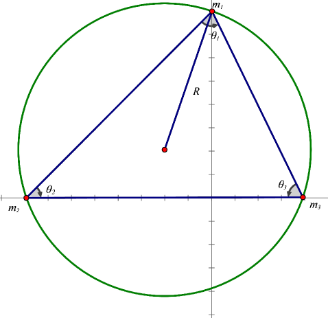
Proposition 6 of [1 ] states that we can have triangular relative equilibria, where the triangle has
any shape. Then we can fix a triangle as a central configuration of the charged three-body problem for some
masses m ∈ ( 𝐑 + ) 3 𝑚 superscript superscript 𝐑 3 m\in({\bf R}^{+})^{3} e ∈ 𝐑 3 𝑒 superscript 𝐑 3 e\in{\bf R}^{3} θ 1 , θ 2 , θ 3 subscript 𝜃 1 subscript 𝜃 2 subscript 𝜃 3
\theta_{1},\theta_{2},\theta_{3}
Figure 2: The nonlinear central configuration of three charged bodies
We have the following theorem.
Theorem 3.1 The linearized system of (1.2 1.3 q ( t ) 𝑞 𝑡 q(t) 2.16
( Z ¯ ˙ z ¯ ˙ W ¯ ˙ w ¯ ˙ ) = ( J B ¯ 1 ( θ ) O O J B ¯ 2 ( θ ) ) ( Z ¯ z ¯ W ¯ w ¯ ) , matrix ˙ ¯ 𝑍 ˙ ¯ 𝑧 ˙ ¯ 𝑊 ˙ ¯ 𝑤 matrix 𝐽 subscript ¯ 𝐵 1 𝜃 𝑂 𝑂 𝐽 subscript ¯ 𝐵 2 𝜃 matrix ¯ 𝑍 ¯ 𝑧 ¯ 𝑊 ¯ 𝑤 \pmatrix{\dot{\bar{Z}}\cr\dot{\bar{z}}\cr\dot{\bar{W}}\cr\dot{\bar{w}}}=\pmatrix{J\bar{B}_{1}(\theta)&O\cr O&J\bar{B}_{2}(\theta)}\pmatrix{\bar{Z}\cr\bar{z}\cr\bar{W}\cr\bar{w}}, (3.1)
where e 𝑒 e
β = 36 α 2 = 36 ( m 2 m 3 sin 2 θ 1 + m 3 m 1 sin 2 θ 2 + m 1 m 2 sin 2 θ 3 ) . 𝛽 36 superscript 𝛼 2 36 subscript 𝑚 2 subscript 𝑚 3 superscript 2 subscript 𝜃 1 subscript 𝑚 3 subscript 𝑚 1 superscript 2 subscript 𝜃 2 subscript 𝑚 1 subscript 𝑚 2 superscript 2 subscript 𝜃 3 \beta=36\alpha^{2}=36(m_{2}m_{3}\sin^{2}\theta_{1}+m_{3}m_{1}\sin^{2}\theta_{2}+m_{1}m_{2}\sin^{2}\theta_{3}). (3.2)
And
( W ¯ ˙ w ¯ ˙ ) = J B ¯ 2 ( θ ) ( W ¯ w ¯ ) matrix ˙ ¯ 𝑊 ˙ ¯ 𝑤 𝐽 subscript ¯ 𝐵 2 𝜃 matrix ¯ 𝑊 ¯ 𝑤 \pmatrix{\dot{\bar{W}}\cr\dot{\bar{w}}}=J\bar{B}_{2}(\theta)\pmatrix{\bar{W}\cr\bar{w}} (3.3)
is the essential part of the linearized system of (3.1
B ¯ 2 ( θ ) = ( 1 0 0 1 0 1 − 1 0 0 − 1 2 e cos θ − 1 − 9 − β 2 ( 1 + e cos θ ) 0 1 0 0 2 e cos θ − 1 + 9 − β 2 ( 1 + e cos θ ) ) , subscript ¯ 𝐵 2 𝜃 matrix 1 0 0 1 0 1 1 0 0 1 2 𝑒 𝜃 1 9 𝛽 2 1 𝑒 𝜃 0 1 0 0 2 𝑒 𝜃 1 9 𝛽 2 1 𝑒 𝜃 \bar{B}_{2}(\theta)=\left(\matrix{1&0&0&1\cr 0&1&-1&0\cr 0&-1&\frac{2e\cos\theta-1-\sqrt{9-\beta}}{2(1+e\cos\theta)}&0\cr 1&0&0&\frac{2e\cos\theta-1+\sqrt{9-\beta}}{2(1+e\cos\theta)}\cr}\right), (3.4)
The rest of this paper focuses on the proof of this theorem.
In [16 ] (cf. p.275), Meyer and Schmidt give the essential part of the fundamental solution of the
elliptic Lagrangian orbit. This method also can be found in [11 ] . For elliptic solutions of the
charged problem, we will follow their method.
Suppose the coordinates of the three particles are given by
a ^ 1 = ( 0 , y ) T , a ^ 2 = ( − x 1 , 0 ) T , a ^ 3 = ( x 2 , 0 ) T , formulae-sequence subscript ^ 𝑎 1 superscript 0 𝑦 𝑇 formulae-sequence subscript ^ 𝑎 2 superscript subscript 𝑥 1 0 𝑇 subscript ^ 𝑎 3 superscript subscript 𝑥 2 0 𝑇 \hat{a}_{1}=(0,y)^{T},\quad\hat{a}_{2}=(-x_{1},0)^{T},\quad\hat{a}_{3}=(x_{2},0)^{T}, (3.5)
where x 1 , x 2 , y > 0 subscript 𝑥 1 subscript 𝑥 2 𝑦
0 x_{1},x_{2},y>0 θ 1 , θ 2 , θ 3 subscript 𝜃 1 subscript 𝜃 2 subscript 𝜃 3
\theta_{1},\theta_{2},\theta_{3} R 𝑅 R
| a ^ 1 − a ^ 2 | = 2 R sin θ 3 , | a ^ 2 − a ^ 3 | = 2 R sin θ 1 , | a ^ 3 − a ^ 1 | = 2 R sin θ 2 , formulae-sequence subscript ^ 𝑎 1 subscript ^ 𝑎 2 2 𝑅 subscript 𝜃 3 formulae-sequence subscript ^ 𝑎 2 subscript ^ 𝑎 3 2 𝑅 subscript 𝜃 1 subscript ^ 𝑎 3 subscript ^ 𝑎 1 2 𝑅 subscript 𝜃 2 |\hat{a}_{1}-\hat{a}_{2}|=2R\sin\theta_{3},\quad|\hat{a}_{2}-\hat{a}_{3}|=2R\sin\theta_{1},\quad|\hat{a}_{3}-\hat{a}_{1}|=2R\sin\theta_{2}, (3.6)
and
a ^ 1 = ( 0 , 2 R sin θ 2 sin θ 3 ) T , a ^ 2 = ( − 2 R cos θ 2 sin θ 3 , 0 ) T , a ^ 3 = ( 2 R sin θ 2 cos θ 3 , 0 ) T . formulae-sequence subscript ^ 𝑎 1 superscript 0 2 𝑅 subscript 𝜃 2 subscript 𝜃 3 𝑇 formulae-sequence subscript ^ 𝑎 2 superscript 2 𝑅 subscript 𝜃 2 subscript 𝜃 3 0 𝑇 subscript ^ 𝑎 3 superscript 2 𝑅 subscript 𝜃 2 subscript 𝜃 3 0 𝑇 \hat{a}_{1}=(0,2R\sin\theta_{2}\sin\theta_{3})^{T},\quad\hat{a}_{2}=(-2R\cos\theta_{2}\sin\theta_{3},0)^{T},\quad\hat{a}_{3}=(2R\sin\theta_{2}\cos\theta_{3},0)^{T}. (3.7)
By (2.17 3.6
sin θ 1 : sin θ 2 : sin θ 3 = δ 23 3 : δ 31 3 : δ 12 3 . : subscript 𝜃 1 subscript 𝜃 2 : subscript 𝜃 3 3 subscript 𝛿 23 : 3 subscript 𝛿 31 : 3 subscript 𝛿 12 \sin\theta_{1}:\sin\theta_{2}:\sin\theta_{3}=\sqrt[3]{\delta_{23}}:\sqrt[3]{\delta_{31}}:\sqrt[3]{\delta_{12}}. (3.8)
Then by (2.21
c ( m ) = m 1 a ^ 1 + m 2 a ^ 2 + m 3 a ^ 3 = ( 2 R ( − m 2 cos θ 2 sin θ 3 + m 3 sin θ 2 cos θ 3 ) 2 R m 1 sin θ 2 sin θ 3 ) . 𝑐 𝑚 subscript 𝑚 1 subscript ^ 𝑎 1 subscript 𝑚 2 subscript ^ 𝑎 2 subscript 𝑚 3 subscript ^ 𝑎 3 matrix 2 𝑅 subscript 𝑚 2 subscript 𝜃 2 subscript 𝜃 3 subscript 𝑚 3 subscript 𝜃 2 subscript 𝜃 3 2 𝑅 subscript 𝑚 1 subscript 𝜃 2 subscript 𝜃 3 c(m)=m_{1}\hat{a}_{1}+m_{2}\hat{a}_{2}+m_{3}\hat{a}_{3}=\pmatrix{2R(-m_{2}\cos\theta_{2}\sin\theta_{3}+m_{3}\sin\theta_{2}\cos\theta_{3})\cr 2Rm_{1}\sin\theta_{2}\sin\theta_{3}}. (3.9)
Let
a i = a ^ i − c ( m ) 2 R α ∀ i = 1 , 2 , 3 , formulae-sequence subscript 𝑎 𝑖 subscript ^ 𝑎 𝑖 𝑐 𝑚 2 𝑅 𝛼 for-all 𝑖 1 2 3
a_{i}=\frac{\hat{a}_{i}-c(m)}{2R\alpha}\quad\quad\forall i=1,2,3, (3.10)
and some α > 0 𝛼 0 \alpha>0 a i subscript 𝑎 𝑖 a_{i}
a 1 subscript 𝑎 1 \displaystyle a_{1} = \displaystyle= 1 α ( m 2 cos θ 2 sin θ 3 − m 3 sin θ 2 cos θ 3 ( m 2 + m 3 ) sin θ 2 sin θ 3 ) , 1 𝛼 matrix subscript 𝑚 2 subscript 𝜃 2 subscript 𝜃 3 subscript 𝑚 3 subscript 𝜃 2 subscript 𝜃 3 subscript 𝑚 2 subscript 𝑚 3 subscript 𝜃 2 subscript 𝜃 3 \displaystyle\frac{1}{\alpha}\pmatrix{m_{2}\cos\theta_{2}\sin\theta_{3}-m_{3}\sin\theta_{2}\cos\theta_{3}\cr(m_{2}+m_{3})\sin\theta_{2}\sin\theta_{3}}, (3.11)
a 2 subscript 𝑎 2 \displaystyle a_{2} = \displaystyle= 1 α ( − ( m 1 + m 3 ) cos θ 2 sin θ 3 − m 3 sin θ 2 cos θ 3 − m 1 sin θ 2 sin θ 3 ) , 1 𝛼 matrix subscript 𝑚 1 subscript 𝑚 3 subscript 𝜃 2 subscript 𝜃 3 subscript 𝑚 3 subscript 𝜃 2 subscript 𝜃 3 subscript 𝑚 1 subscript 𝜃 2 subscript 𝜃 3 \displaystyle\frac{1}{\alpha}\pmatrix{-(m_{1}+m_{3})\cos\theta_{2}\sin\theta_{3}-m_{3}\sin\theta_{2}\cos\theta_{3}\cr-m_{1}\sin\theta_{2}\sin\theta_{3}}, (3.12)
= \displaystyle= 1 α ( − m 1 cos θ 2 sin θ 3 − m 3 sin ( θ 2 + θ 3 ) − m 1 sin θ 2 sin θ 3 ) , 1 𝛼 matrix subscript 𝑚 1 subscript 𝜃 2 subscript 𝜃 3 subscript 𝑚 3 subscript 𝜃 2 subscript 𝜃 3 subscript 𝑚 1 subscript 𝜃 2 subscript 𝜃 3 \displaystyle\frac{1}{\alpha}\pmatrix{-m_{1}\cos\theta_{2}\sin\theta_{3}-m_{3}\sin(\theta_{2}+\theta_{3})\cr-m_{1}\sin\theta_{2}\sin\theta_{3}},
a 3 subscript 𝑎 3 \displaystyle a_{3} = \displaystyle= 1 α ( m 2 cos θ 2 sin θ 3 + ( m 1 + m 2 ) sin θ 2 cos θ 3 − m 1 sin θ 2 sin θ 3 ) 1 𝛼 matrix subscript 𝑚 2 subscript 𝜃 2 subscript 𝜃 3 subscript 𝑚 1 subscript 𝑚 2 subscript 𝜃 2 subscript 𝜃 3 subscript 𝑚 1 subscript 𝜃 2 subscript 𝜃 3 \displaystyle\frac{1}{\alpha}\pmatrix{m_{2}\cos\theta_{2}\sin\theta_{3}+(m_{1}+m_{2})\sin\theta_{2}\cos\theta_{3}\cr-m_{1}\sin\theta_{2}\sin\theta_{3}} (3.13)
= \displaystyle= 1 α ( m 2 sin ( θ 2 + θ 3 ) + m 1 sin θ 2 cos θ 3 − m 1 sin θ 2 sin θ 3 ) . 1 𝛼 matrix subscript 𝑚 2 subscript 𝜃 2 subscript 𝜃 3 subscript 𝑚 1 subscript 𝜃 2 subscript 𝜃 3 subscript 𝑚 1 subscript 𝜃 2 subscript 𝜃 3 \displaystyle\frac{1}{\alpha}\pmatrix{m_{2}\sin(\theta_{2}+\theta_{3})+m_{1}\sin\theta_{2}\cos\theta_{3}\cr-m_{1}\sin\theta_{2}\sin\theta_{3}}.
To determine α 𝛼 \alpha a i subscript 𝑎 𝑖 a_{i} 2.21
θ 1 + θ 2 + θ 3 = π , subscript 𝜃 1 subscript 𝜃 2 subscript 𝜃 3 𝜋 \theta_{1}+\theta_{2}+\theta_{3}=\pi, (3.14)
which yield
1 1 \displaystyle 1 = \displaystyle= m 1 | a 1 | 2 + m 2 | a 2 | 2 + m 3 | a 3 | 2 subscript 𝑚 1 superscript subscript 𝑎 1 2 subscript 𝑚 2 superscript subscript 𝑎 2 2 subscript 𝑚 3 superscript subscript 𝑎 3 2 \displaystyle m_{1}|a_{1}|^{2}+m_{2}|a_{2}|^{2}+m_{3}|a_{3}|^{2} (3.15)
= \displaystyle= 1 α 2 [ m 1 ( m 2 2 sin 2 θ 3 + m 3 2 sin 2 θ 2 − 2 m 2 m 3 sin θ 2 sin θ 3 cos ( θ 2 + θ 3 ) ) \displaystyle\frac{1}{\alpha^{2}}[m_{1}(m_{2}^{2}\sin^{2}\theta_{3}+m_{3}^{2}\sin^{2}\theta_{2}-2m_{2}m_{3}\sin\theta_{2}\sin\theta_{3}\cos(\theta_{2}+\theta_{3}))
+ m 2 ( m 1 2 sin 2 θ 3 + m 3 2 sin 2 ( θ 2 + θ 3 ) + 2 m 3 m 1 sin ( θ 2 + θ 3 ) cos θ 2 sin θ 3 ) subscript 𝑚 2 superscript subscript 𝑚 1 2 superscript 2 subscript 𝜃 3 superscript subscript 𝑚 3 2 superscript 2 subscript 𝜃 2 subscript 𝜃 3 2 subscript 𝑚 3 subscript 𝑚 1 subscript 𝜃 2 subscript 𝜃 3 subscript 𝜃 2 subscript 𝜃 3 \displaystyle\quad+m_{2}(m_{1}^{2}\sin^{2}\theta_{3}+m_{3}^{2}\sin^{2}(\theta_{2}+\theta_{3})+2m_{3}m_{1}\sin(\theta_{2}+\theta_{3})\cos\theta_{2}\sin\theta_{3})
+ m 3 ( m 1 2 sin 2 θ 2 + m 2 2 sin 2 ( θ 2 + θ 3 ) + 2 m 1 m 2 sin ( θ 2 + θ 3 ) sin θ 2 cos θ 3 ) ] \displaystyle\quad+m_{3}(m_{1}^{2}\sin^{2}\theta_{2}+m_{2}^{2}\sin^{2}(\theta_{2}+\theta_{3})+2m_{1}m_{2}\sin(\theta_{2}+\theta_{3})\sin\theta_{2}\cos\theta_{3})]
= \displaystyle= 1 α 2 [ m 2 m 3 ( m 2 + m 3 ) sin 2 θ 1 + m 3 m 1 ( m 3 + m 1 ) sin 2 θ 2 + m 1 m 2 ( m 1 + m 2 ) sin 2 θ 3 \displaystyle\frac{1}{\alpha^{2}}[m_{2}m_{3}(m_{2}+m_{3})\sin^{2}\theta_{1}+m_{3}m_{1}(m_{3}+m_{1})\sin^{2}\theta_{2}+m_{1}m_{2}(m_{1}+m_{2})\sin^{2}\theta_{3}
+ 2 m 1 m 2 m 3 ( cos θ 1 sin θ 2 sin θ 3 + sin θ 1 cos θ 2 sin θ 3 + sin θ 1 sin θ 2 cos θ 3 ) ] \displaystyle\quad+2m_{1}m_{2}m_{3}(\cos\theta_{1}\sin\theta_{2}\sin\theta_{3}+\sin\theta_{1}\cos\theta_{2}\sin\theta_{3}+\sin\theta_{1}\sin\theta_{2}\cos\theta_{3})]
= \displaystyle= 1 α 2 [ m 2 m 3 ( 1 − m 1 ) sin 2 θ 1 + m 3 m 1 ( 1 − m 2 ) sin 2 θ 2 + m 1 m 2 ( 1 − m 3 ) sin 2 θ 3 \displaystyle\frac{1}{\alpha^{2}}[m_{2}m_{3}(1-m_{1})\sin^{2}\theta_{1}+m_{3}m_{1}(1-m_{2})\sin^{2}\theta_{2}+m_{1}m_{2}(1-m_{3})\sin^{2}\theta_{3}
+ 2 m 1 m 2 m 3 ( cos θ 1 sin θ 2 sin θ 3 + sin θ 1 cos θ 2 sin θ 3 + sin θ 1 sin θ 2 cos θ 3 ) ] \displaystyle\quad+2m_{1}m_{2}m_{3}(\cos\theta_{1}\sin\theta_{2}\sin\theta_{3}+\sin\theta_{1}\cos\theta_{2}\sin\theta_{3}+\sin\theta_{1}\sin\theta_{2}\cos\theta_{3})]
= \displaystyle= 1 α 2 [ m 2 m 3 sin 2 θ 1 + m 3 m 1 sin 2 θ 2 + m 1 m 2 sin 2 θ 3 ] 1 superscript 𝛼 2 delimited-[] subscript 𝑚 2 subscript 𝑚 3 superscript 2 subscript 𝜃 1 subscript 𝑚 3 subscript 𝑚 1 superscript 2 subscript 𝜃 2 subscript 𝑚 1 subscript 𝑚 2 superscript 2 subscript 𝜃 3 \displaystyle\frac{1}{\alpha^{2}}[m_{2}m_{3}\sin^{2}\theta_{1}+m_{3}m_{1}\sin^{2}\theta_{2}+m_{1}m_{2}\sin^{2}\theta_{3}]
+ m 1 m 2 m 3 α 2 [ 2 cos θ 1 sin θ 2 sin θ 3 + 2 sin θ 1 cos θ 2 sin θ 3 + 2 sin θ 1 sin θ 2 cos θ 3 \displaystyle+\frac{m_{1}m_{2}m_{3}}{\alpha^{2}}[2\cos\theta_{1}\sin\theta_{2}\sin\theta_{3}+2\sin\theta_{1}\cos\theta_{2}\sin\theta_{3}+2\sin\theta_{1}\sin\theta_{2}\cos\theta_{3}
− ( sin 2 θ 1 + sin 2 θ 2 + sin 2 θ 3 ) ] \displaystyle\quad\quad\quad\quad-(\sin^{2}\theta_{1}+\sin^{2}\theta_{2}+\sin^{2}\theta_{3})]
= \displaystyle= 1 α 2 [ m 2 m 3 sin 2 θ 1 + m 3 m 1 sin 2 θ 2 + m 1 m 2 sin 2 θ 3 ] , 1 superscript 𝛼 2 delimited-[] subscript 𝑚 2 subscript 𝑚 3 superscript 2 subscript 𝜃 1 subscript 𝑚 3 subscript 𝑚 1 superscript 2 subscript 𝜃 2 subscript 𝑚 1 subscript 𝑚 2 superscript 2 subscript 𝜃 3 \displaystyle\frac{1}{\alpha^{2}}[m_{2}m_{3}\sin^{2}\theta_{1}+m_{3}m_{1}\sin^{2}\theta_{2}+m_{1}m_{2}\sin^{2}\theta_{3}],
where in the last equality, we used
2 cos θ 1 sin θ 2 sin θ 3 + 2 sin θ 1 cos θ 2 sin θ 3 + 2 sin θ 1 sin θ 2 cos θ 3 2 subscript 𝜃 1 subscript 𝜃 2 subscript 𝜃 3 2 subscript 𝜃 1 subscript 𝜃 2 subscript 𝜃 3 2 subscript 𝜃 1 subscript 𝜃 2 subscript 𝜃 3 \displaystyle 2\cos\theta_{1}\sin\theta_{2}\sin\theta_{3}+2\sin\theta_{1}\cos\theta_{2}\sin\theta_{3}+2\sin\theta_{1}\sin\theta_{2}\cos\theta_{3}
= sin θ 1 ( cos θ 2 sin θ 3 + sin θ 2 cos θ 3 ) + sin θ 2 ( cos θ 1 sin θ 3 + sin θ 1 cos θ 3 ) absent subscript 𝜃 1 subscript 𝜃 2 subscript 𝜃 3 subscript 𝜃 2 subscript 𝜃 3 subscript 𝜃 2 subscript 𝜃 1 subscript 𝜃 3 subscript 𝜃 1 subscript 𝜃 3 \displaystyle\quad=\sin\theta_{1}(\cos\theta_{2}\sin\theta_{3}+\sin\theta_{2}\cos\theta_{3})+\sin\theta_{2}(\cos\theta_{1}\sin\theta_{3}+\sin\theta_{1}\cos\theta_{3})
+ sin θ 3 ( cos θ 1 sin θ 2 + sin θ 1 cos θ 2 ) subscript 𝜃 3 subscript 𝜃 1 subscript 𝜃 2 subscript 𝜃 1 subscript 𝜃 2 \displaystyle\quad\qquad+\sin\theta_{3}(\cos\theta_{1}\sin\theta_{2}+\sin\theta_{1}\cos\theta_{2})
= sin θ 1 sin ( θ 2 + θ 3 ) + sin θ 2 sin ( θ 1 + θ 3 ) + sin θ 3 sin ( θ 1 + θ 2 ) absent subscript 𝜃 1 subscript 𝜃 2 subscript 𝜃 3 subscript 𝜃 2 subscript 𝜃 1 subscript 𝜃 3 subscript 𝜃 3 subscript 𝜃 1 subscript 𝜃 2 \displaystyle\quad=\sin\theta_{1}\sin(\theta_{2}+\theta_{3})+\sin\theta_{2}\sin(\theta_{1}+\theta_{3})+\sin\theta_{3}\sin(\theta_{1}+\theta_{2})
= sin 2 θ 1 + sin 2 θ 2 + sin 2 θ 3 . absent superscript 2 subscript 𝜃 1 superscript 2 subscript 𝜃 2 superscript 2 subscript 𝜃 3 \displaystyle\quad=\sin^{2}\theta_{1}+\sin^{2}\theta_{2}+\sin^{2}\theta_{3}. (3.16)
Thus we define
α = m 2 m 3 sin 2 θ 1 + m 3 m 1 sin 2 θ 2 + m 1 m 2 sin 2 θ 3 . 𝛼 subscript 𝑚 2 subscript 𝑚 3 superscript 2 subscript 𝜃 1 subscript 𝑚 3 subscript 𝑚 1 superscript 2 subscript 𝜃 2 subscript 𝑚 1 subscript 𝑚 2 superscript 2 subscript 𝜃 3 \alpha=\sqrt{m_{2}m_{3}\sin^{2}\theta_{1}+m_{3}m_{1}\sin^{2}\theta_{2}+m_{1}m_{2}\sin^{2}\theta_{3}}. (3.17)
Now as in p.263 of [16 ] , Section 11.2 of [11 ] , we define
P = ( p 1 p 2 p 3 ) , Q = ( q 1 q 2 q 3 ) , Y = ( G Z W ) , X = ( g z w ) , formulae-sequence 𝑃 matrix subscript 𝑝 1 subscript 𝑝 2 subscript 𝑝 3 formulae-sequence 𝑄 matrix subscript 𝑞 1 subscript 𝑞 2 subscript 𝑞 3 formulae-sequence 𝑌 matrix 𝐺 𝑍 𝑊 𝑋 matrix 𝑔 𝑧 𝑤 P=\left(\matrix{p_{1}\cr p_{2}\cr p_{3}}\right),\quad Q=\left(\matrix{q_{1}\cr q_{2}\cr q_{3}}\right),\quad Y=\left(\matrix{G\cr Z\cr W}\right),\quad X=\left(\matrix{g\cr z\cr w}\right), (3.18)
where p i subscript 𝑝 𝑖 p_{i} q i subscript 𝑞 𝑖 q_{i} i = 1 , 2 , 3 𝑖 1 2 3
i=1,2,3 G 𝐺 G Z 𝑍 Z W 𝑊 W g 𝑔 g z 𝑧 z w 𝑤 w 𝐑 2 superscript 𝐑 2 {\bf R}^{2}
P = A − T Y , Q = A X , formulae-sequence 𝑃 superscript 𝐴 𝑇 𝑌 𝑄 𝐴 𝑋 P=A^{-T}Y,\quad Q=AX, (3.19)
where the matrix A 𝐴 A [16 ] . Concretely, the matrix
A ∈ 𝐆𝐋 ( 𝐑 6 ) 𝐴 𝐆𝐋 superscript 𝐑 6 A\in{\bf GL}({\bf R}^{6})
A = ( I A 1 B 1 I A 2 B 2 I A 3 B 3 ) , 𝐴 matrix 𝐼 subscript 𝐴 1 subscript 𝐵 1
𝐼 subscript 𝐴 2 subscript 𝐵 2
𝐼 subscript 𝐴 3 subscript 𝐵 3
A=\left(\matrix{I\quad A_{1}\quad B_{1}\cr I\quad A_{2}\quad B_{2}\cr I\quad A_{3}\quad B_{3}}\right), (3.20)
as each A i subscript 𝐴 𝑖 A_{i} 2 × 2 2 2 2\times 2
A 1 subscript 𝐴 1 \displaystyle A_{1} = \displaystyle= ( a 1 , J a 1 ) = ( m 2 cos θ 2 sin θ 3 − m 3 sin θ 2 cos θ 3 α − ( m 2 + m 3 ) sin θ 2 sin θ 3 α ( m 2 + m 3 ) sin θ 2 sin θ 3 α m 2 cos θ 2 sin θ 3 − m 3 sin θ 2 cos θ 3 α ) , subscript 𝑎 1 𝐽 subscript 𝑎 1 matrix subscript 𝑚 2 subscript 𝜃 2 subscript 𝜃 3 subscript 𝑚 3 subscript 𝜃 2 subscript 𝜃 3 𝛼 subscript 𝑚 2 subscript 𝑚 3 subscript 𝜃 2 subscript 𝜃 3 𝛼 subscript 𝑚 2 subscript 𝑚 3 subscript 𝜃 2 subscript 𝜃 3 𝛼 subscript 𝑚 2 subscript 𝜃 2 subscript 𝜃 3 subscript 𝑚 3 subscript 𝜃 2 subscript 𝜃 3 𝛼 \displaystyle(a_{1},Ja_{1})=\pmatrix{\frac{m_{2}\cos\theta_{2}\sin\theta_{3}-m_{3}\sin\theta_{2}\cos\theta_{3}}{\alpha}&-\frac{(m_{2}+m_{3})\sin\theta_{2}\sin\theta_{3}}{\alpha}\cr\frac{(m_{2}+m_{3})\sin\theta_{2}\sin\theta_{3}}{\alpha}&\frac{m_{2}\cos\theta_{2}\sin\theta_{3}-m_{3}\sin\theta_{2}\cos\theta_{3}}{\alpha}}, (3.21)
A 2 subscript 𝐴 2 \displaystyle A_{2} = \displaystyle= ( a 2 , J a 2 ) = ( − m 1 cos θ 2 sin θ 3 + m 3 sin ( θ 2 + θ 3 ) α m 1 sin θ 2 sin θ 3 α − m 1 sin θ 2 sin θ 3 α − m 1 cos θ 2 sin θ 3 + m 3 sin ( θ 2 + θ 3 ) α ) , subscript 𝑎 2 𝐽 subscript 𝑎 2 matrix subscript 𝑚 1 subscript 𝜃 2 subscript 𝜃 3 subscript 𝑚 3 subscript 𝜃 2 subscript 𝜃 3 𝛼 subscript 𝑚 1 subscript 𝜃 2 subscript 𝜃 3 𝛼 subscript 𝑚 1 subscript 𝜃 2 subscript 𝜃 3 𝛼 subscript 𝑚 1 subscript 𝜃 2 subscript 𝜃 3 subscript 𝑚 3 subscript 𝜃 2 subscript 𝜃 3 𝛼 \displaystyle(a_{2},Ja_{2})=\pmatrix{-\frac{m_{1}\cos\theta_{2}\sin\theta_{3}+m_{3}\sin(\theta_{2}+\theta_{3})}{\alpha}&\frac{m_{1}\sin\theta_{2}\sin\theta_{3}}{\alpha}\cr-\frac{m_{1}\sin\theta_{2}\sin\theta_{3}}{\alpha}&-\frac{m_{1}\cos\theta_{2}\sin\theta_{3}+m_{3}\sin(\theta_{2}+\theta_{3})}{\alpha}}, (3.22)
A 3 subscript 𝐴 3 \displaystyle A_{3} = \displaystyle= ( a 3 , J a 3 ) = ( m 2 sin ( θ 2 + θ 3 ) + m 1 sin θ 2 cos θ 3 α m 1 sin θ 2 sin θ 3 α − m 1 sin θ 2 sin θ 3 α m 2 sin ( θ 2 + θ 3 ) + m 1 sin θ 2 cos θ 3 α ) . subscript 𝑎 3 𝐽 subscript 𝑎 3 matrix subscript 𝑚 2 subscript 𝜃 2 subscript 𝜃 3 subscript 𝑚 1 subscript 𝜃 2 subscript 𝜃 3 𝛼 subscript 𝑚 1 subscript 𝜃 2 subscript 𝜃 3 𝛼 subscript 𝑚 1 subscript 𝜃 2 subscript 𝜃 3 𝛼 subscript 𝑚 2 subscript 𝜃 2 subscript 𝜃 3 subscript 𝑚 1 subscript 𝜃 2 subscript 𝜃 3 𝛼 \displaystyle(a_{3},Ja_{3})=\pmatrix{\frac{m_{2}\sin(\theta_{2}+\theta_{3})+m_{1}\sin\theta_{2}\cos\theta_{3}}{\alpha}&\frac{m_{1}\sin\theta_{2}\sin\theta_{3}}{\alpha}\cr-\frac{m_{1}\sin\theta_{2}\sin\theta_{3}}{\alpha}&\frac{m_{2}\sin(\theta_{2}+\theta_{3})+m_{1}\sin\theta_{2}\cos\theta_{3}}{\alpha}}. (3.23)
To fulfill A T M A = I superscript 𝐴 𝑇 𝑀 𝐴 𝐼 A^{T}MA=I [16 ] ), we must have
B 1 subscript 𝐵 1 \displaystyle B_{1} = \displaystyle= ρ 1 ( A 3 − A 2 ) T = ρ 1 sin θ 1 α I , subscript 𝜌 1 superscript subscript 𝐴 3 subscript 𝐴 2 𝑇 subscript 𝜌 1 subscript 𝜃 1 𝛼 𝐼 \displaystyle\rho_{1}(A_{3}-A_{2})^{T}=\frac{\rho_{1}\sin\theta_{1}}{\alpha}I, (3.24)
B 2 subscript 𝐵 2 \displaystyle B_{2} = \displaystyle= ρ 2 ( A 1 − A 3 ) T = − ρ 2 sin θ 2 α R ( θ 3 ) , subscript 𝜌 2 superscript subscript 𝐴 1 subscript 𝐴 3 𝑇 subscript 𝜌 2 subscript 𝜃 2 𝛼 𝑅 subscript 𝜃 3 \displaystyle\rho_{2}(A_{1}-A_{3})^{T}=-\frac{\rho_{2}\sin\theta_{2}}{\alpha}R(\theta_{3}), (3.25)
B 3 subscript 𝐵 3 \displaystyle B_{3} = \displaystyle= ρ 3 ( A 2 − A 1 ) T = − ρ 3 sin θ 3 α R ( − θ 2 ) , subscript 𝜌 3 superscript subscript 𝐴 2 subscript 𝐴 1 𝑇 subscript 𝜌 3 subscript 𝜃 3 𝛼 𝑅 subscript 𝜃 2 \displaystyle\rho_{3}(A_{2}-A_{1})^{T}=-\frac{\rho_{3}\sin\theta_{3}}{\alpha}R(-\theta_{2}), (3.26)
where
ρ i = m 1 m 2 m 3 m i , ∀ 1 ≤ i ≤ 3 . formulae-sequence subscript 𝜌 𝑖 subscript 𝑚 1 subscript 𝑚 2 subscript 𝑚 3 subscript 𝑚 𝑖 for-all 1 𝑖 3 \rho_{i}=\frac{\sqrt{m_{1}m_{2}m_{3}}}{m_{i}},\quad\forall 1\leq i\leq 3. (3.27)
Moreover, from (3.24 3.26
B i B j = B j B i ∀ 1 ≤ i , j ≤ 3 . formulae-sequence subscript 𝐵 𝑖 subscript 𝐵 𝑗 subscript 𝐵 𝑗 subscript 𝐵 𝑖 formulae-sequence for-all 1 𝑖 𝑗 3 B_{i}B_{j}=B_{j}B_{i}\quad\quad\forall 1\leq i,j\leq 3. (3.28)
Under the coordinate change (3.19
K = 1 2 ( | G | 2 + | Z | 2 + | W | 2 ) , 𝐾 1 2 superscript 𝐺 2 superscript 𝑍 2 superscript 𝑊 2 K=\frac{1}{2}(|G|^{2}+|Z|^{2}+|W|^{2}), (3.29)
and the potential function
U ( z , w ) = ∑ 1 ≤ i < j ≤ 3 m i m j − e i e j d i j ( z , w ) = ∑ 1 ≤ i < j ≤ 3 m i m j δ i j d i j ( z , w ) , 𝑈 𝑧 𝑤 subscript 1 𝑖 𝑗 3 subscript 𝑚 𝑖 subscript 𝑚 𝑗 subscript 𝑒 𝑖 subscript 𝑒 𝑗 subscript 𝑑 𝑖 𝑗 𝑧 𝑤 subscript 1 𝑖 𝑗 3 subscript 𝑚 𝑖 subscript 𝑚 𝑗 subscript 𝛿 𝑖 𝑗 subscript 𝑑 𝑖 𝑗 𝑧 𝑤 U(z,w)=\sum_{1\leq i<j\leq 3}\frac{m_{i}m_{j}-e_{i}e_{j}}{d_{ij}(z,w)}=\sum_{1\leq i<j\leq 3}\frac{m_{i}m_{j}\delta_{ij}}{d_{ij}(z,w)}, (3.30)
with
d i j ( z , w ) = | ( A i − A j ) z + ( B i − B j ) w | ∀ 1 ≤ i < j ≤ 3 . formulae-sequence subscript 𝑑 𝑖 𝑗 𝑧 𝑤 subscript 𝐴 𝑖 subscript 𝐴 𝑗 𝑧 subscript 𝐵 𝑖 subscript 𝐵 𝑗 𝑤 for-all 1 𝑖 𝑗 3 d_{ij}(z,w)=|(A_{i}-A_{j})z+(B_{i}-B_{j})w|\quad\quad\quad\forall 1\leq i<j\leq 3. (3.31)
Let θ 𝜃 \theta [16 ] (also in Theorem 11.10 of [11 ] ), the resulting Hamiltonian function of the charged 3-body problem
is given by
H ( θ , Z ¯ , W ¯ , z ¯ , w ¯ ) = 1 2 ( | Z ¯ | 2 + | W ¯ | 2 ) + ( z ¯ ⋅ J Z ¯ + w ¯ ⋅ J W ¯ ) + p − r ( θ ) 2 p ( | z ¯ | 2 + | w ¯ | 2 ) − r ( θ ) ( μ p ) 1 / 4 , 𝐻 𝜃 ¯ 𝑍 ¯ 𝑊 ¯ 𝑧 ¯ 𝑤 1 2 superscript ¯ 𝑍 2 superscript ¯ 𝑊 2 ⋅ ¯ 𝑧 𝐽 ¯ 𝑍 ⋅ ¯ 𝑤 𝐽 ¯ 𝑊 𝑝 𝑟 𝜃 2 𝑝 superscript ¯ 𝑧 2 superscript ¯ 𝑤 2 𝑟 𝜃 superscript 𝜇 𝑝 1 4 H(\theta,\bar{Z},\bar{W},\bar{z},\bar{w})=\frac{1}{2}(|\bar{Z}|^{2}+|\bar{W}|^{2})+(\bar{z}\cdot J\bar{Z}+\bar{w}\cdot J\bar{W})+\frac{p-r(\theta)}{2p}(|\bar{z}|^{2}+|\bar{w}|^{2})-\frac{r(\theta)}{(\mu p)^{1/4}}, (3.32)
where
r ( θ ) = p 1 + e cos θ 𝑟 𝜃 𝑝 1 𝑒 𝜃 r(\theta)=\frac{p}{1+e\cos\theta} (3.33)
and μ 𝜇 \mu 2.6 ( μ p ) 1 / 4 superscript 𝜇 𝑝 1 4 (\mu p)^{1/4} p > 0 𝑝 0 p>0 μ > 0 𝜇 0 \mu>0 2.17
k = δ 12 3 | a 1 − a 2 | = δ 23 3 | a 2 − a 3 | = δ 31 3 | a 3 − a 1 | , 𝑘 3 subscript 𝛿 12 subscript 𝑎 1 subscript 𝑎 2 3 subscript 𝛿 23 subscript 𝑎 2 subscript 𝑎 3 3 subscript 𝛿 31 subscript 𝑎 3 subscript 𝑎 1 k=\frac{\sqrt[3]{\delta_{12}}}{|a_{1}-a_{2}|}=\frac{\sqrt[3]{\delta_{23}}}{|a_{2}-a_{3}|}=\frac{\sqrt[3]{\delta_{31}}}{|a_{3}-a_{1}|}, (3.34)
then together with (3.6 3.10
δ i j = k 3 sin 3 θ l α 3 , | a i − a j | = sin θ l α , formulae-sequence subscript 𝛿 𝑖 𝑗 superscript 𝑘 3 superscript 3 subscript 𝜃 𝑙 superscript 𝛼 3 subscript 𝑎 𝑖 subscript 𝑎 𝑗 subscript 𝜃 𝑙 𝛼 \delta_{ij}=\frac{k^{3}\sin^{3}\theta_{l}}{\alpha^{3}},\quad|a_{i}-a_{j}|=\frac{\sin\theta_{l}}{\alpha}, (3.35)
where { i , j , l } 𝑖 𝑗 𝑙 \{i,j,l\} { 1 , 2 , 3 } 1 2 3 \{1,2,3\} 2.6 3.35
μ = ∑ 1 ≤ i < j ≤ 3 , l ≠ i , j m i m j k 3 sin 2 θ l α 2 = k 3 α 2 ∑ 1 ≤ i < j ≤ 3 , l ≠ i , j m i m j sin 2 θ l = k 3 , 𝜇 subscript formulae-sequence 1 𝑖 𝑗 3 𝑙 𝑖 𝑗
subscript 𝑚 𝑖 subscript 𝑚 𝑗 superscript 𝑘 3 superscript 2 subscript 𝜃 𝑙 superscript 𝛼 2 superscript 𝑘 3 superscript 𝛼 2 subscript formulae-sequence 1 𝑖 𝑗 3 𝑙 𝑖 𝑗
subscript 𝑚 𝑖 subscript 𝑚 𝑗 superscript 2 subscript 𝜃 𝑙 superscript 𝑘 3 \mu=\sum_{1\leq i<j\leq 3,\ l\neq i,j}m_{i}m_{j}\frac{k^{3}\sin^{2}\theta_{l}}{\alpha^{2}}=\frac{k^{3}}{\alpha^{2}}\sum_{1\leq i<j\leq 3,\ l\neq i,j}m_{i}m_{j}\sin^{2}\theta_{l}=k^{3}, (3.36)
where we used (3.17
Based on Lemma 3.1 in [16 ] , we now derive the transformed version of the elliptic triangle
solutions and the linearized Hamiltonian system at such solutions. Let σ = ( p μ ) 1 / 4 𝜎 superscript 𝑝 𝜇 1 4 {\sigma}=(p\mu)^{1/4} M = diag ( m 1 I , m 2 I , m 3 I ) 𝑀 diag subscript 𝑚 1 𝐼 subscript 𝑚 2 𝐼 subscript 𝑚 3 𝐼 M={\rm diag}(m_{1}I,m_{2}I,m_{3}I) 2.1 n = 3 𝑛 3 n=3 k = 2 𝑘 2 k=2
Proposition 3.2 Using notations (3.18 ( P ( t ) , Q ( t ) ) T superscript 𝑃 𝑡 𝑄 𝑡 𝑇 (P(t),Q(t))^{T} 1.2
Q ( t ) = ( r ( t ) R ( θ ( t ) ) a 1 , r ( t ) R ( θ ( t ) ) a 2 , r ( t ) R ( θ ( t ) ) a 3 ) T , P ( t ) = M Q ˙ ( t ) formulae-sequence 𝑄 𝑡 superscript 𝑟 𝑡 𝑅 𝜃 𝑡 subscript 𝑎 1 𝑟 𝑡 𝑅 𝜃 𝑡 subscript 𝑎 2 𝑟 𝑡 𝑅 𝜃 𝑡 subscript 𝑎 3 𝑇 𝑃 𝑡 𝑀 ˙ 𝑄 𝑡 Q(t)=(r(t)R({\theta}(t))a_{1},r(t)R({\theta}(t))a_{2},r(t)R({\theta}(t))a_{3})^{T},\quad P(t)=M\dot{Q}(t) (3.37)
in the variable of time t 𝑡 t ( Y ( θ ) , X ( θ ) ) T superscript 𝑌 𝜃 𝑋 𝜃 𝑇 (Y({\theta}),X({\theta}))^{T} θ 𝜃 {\theta} G ≡ g ≡ 0 𝐺 𝑔 0 G\equiv g\equiv 0 H 𝐻 H 3.32
Y ( θ ) = ( Z ¯ ( θ ) W ¯ ( θ ) ) = ( 0 σ 0 0 ) , X ( θ ) = ( z ¯ ( θ ) w ¯ ( θ ) ) = ( σ 0 0 0 ) . formulae-sequence 𝑌 𝜃 matrix ¯ 𝑍 𝜃 ¯ 𝑊 𝜃 matrix 0 𝜎 0 0 𝑋 𝜃 matrix ¯ 𝑧 𝜃 ¯ 𝑤 𝜃 matrix 𝜎 0 0 0 Y({\theta})=\left(\matrix{\bar{Z}({\theta})\cr\bar{W}({\theta})\cr}\right)=\left(\matrix{0\cr{\sigma}\cr 0\cr 0\cr}\right),\quad X({\theta})=\left(\matrix{\bar{z}({\theta})\cr\bar{w}({\theta})\cr}\right)=\left(\matrix{{\sigma}\cr 0\cr 0\cr 0\cr}\right). (3.38)
Proof. By transformation (3.19 ( P ( t ) , Q ( t ) ) T superscript 𝑃 𝑡 𝑄 𝑡 𝑇 (P(t),Q(t))^{T} 3.37 ( 0 , Z ( t ) , 0 , 0 , z ( t ) , 0 ) T superscript 0 𝑍 𝑡 0 0 𝑧 𝑡 0 𝑇 (0,Z(t),0,0,z(t),0)^{T}
H = 1 2 ( Z 1 2 + Z 2 2 + W 1 2 + W 2 2 ) − U ( z , w ) , 𝐻 1 2 superscript subscript 𝑍 1 2 superscript subscript 𝑍 2 2 superscript subscript 𝑊 1 2 superscript subscript 𝑊 2 2 𝑈 𝑧 𝑤 H=\frac{1}{2}(Z_{1}^{2}+Z_{2}^{2}+W_{1}^{2}+W_{2}^{2})-U(z,w), (3.39)
where
z ( t ) = ( r ( t ) cos θ ( t ) r ( t ) sin θ ( t ) ) and Z ( t ) = R ( θ ( t ) ) ( r ˙ ( t ) r ( t ) θ ˙ ( t ) ) . formulae-sequence 𝑧 𝑡 matrix 𝑟 𝑡 𝜃 𝑡 𝑟 𝑡 𝜃 𝑡 and
𝑍 𝑡 𝑅 𝜃 𝑡 matrix ˙ 𝑟 𝑡 𝑟 𝑡 ˙ 𝜃 𝑡 z(t)=\left(\matrix{r(t)\cos{\theta}(t)\cr r(t)\sin{\theta}(t)\cr}\right)\quad{\rm and}\quad Z(t)=R({\theta}(t))\left(\matrix{\dot{r}(t)\cr r(t)\dot{{\theta}}(t)\cr}\right). (3.40)
Then setting G = g = 0 𝐺 𝑔 0 G=g=0 [16 ] , the solution ( Z ( t ) , 0 , z ( t ) , 0 ) T superscript 𝑍 𝑡 0 𝑧 𝑡 0 𝑇 (Z(t),0,z(t),0)^{T} 3.39 ( Z ~ , 0 , z ~ , 0 ) T superscript ~ 𝑍 0 ~ 𝑧 0 𝑇 (\tilde{Z},0,\tilde{z},0)^{T}
H = 1 2 ( Z ~ 1 2 + Z ~ 2 2 + W ~ 1 2 + W ~ 2 2 ) + ( z ~ 2 Z ~ 1 − z ~ 1 Z ~ 2 + w ~ 2 W ~ 1 − w ~ 1 W ~ 2 ) θ ˙ − U ( z ~ , w ~ ) , 𝐻 1 2 superscript subscript ~ 𝑍 1 2 superscript subscript ~ 𝑍 2 2 superscript subscript ~ 𝑊 1 2 superscript subscript ~ 𝑊 2 2 subscript ~ 𝑧 2 subscript ~ 𝑍 1 subscript ~ 𝑧 1 subscript ~ 𝑍 2 subscript ~ 𝑤 2 subscript ~ 𝑊 1 subscript ~ 𝑤 1 subscript ~ 𝑊 2 ˙ 𝜃 𝑈 ~ 𝑧 ~ 𝑤 H=\frac{1}{2}(\tilde{Z}_{1}^{2}+\tilde{Z}_{2}^{2}+\tilde{W}_{1}^{2}+\tilde{W}_{2}^{2})+(\tilde{z}_{2}\tilde{Z}_{1}-\tilde{z}_{1}\tilde{Z}_{2}+\tilde{w}_{2}\tilde{W}_{1}-\tilde{w}_{1}\tilde{W}_{2})\dot{\theta}-U(\tilde{z},\tilde{w}), (3.41)
where
z ~ ( t ) = R ( θ ( t ) ) T z ( t ) = ( r ( t ) 0 ) , Z ~ ( t ) = R ( θ ( t ) ) T Z ( t ) = ( r ˙ ( t ) r ( t ) θ ˙ ( t ) ) . formulae-sequence ~ 𝑧 𝑡 𝑅 superscript 𝜃 𝑡 𝑇 𝑧 𝑡 matrix 𝑟 𝑡 0 ~ 𝑍 𝑡 𝑅 superscript 𝜃 𝑡 𝑇 𝑍 𝑡 matrix ˙ 𝑟 𝑡 𝑟 𝑡 ˙ 𝜃 𝑡 \tilde{z}(t)=R({\theta}(t))^{T}z(t)=\left(\matrix{r(t)\cr 0\cr}\right),\quad\tilde{Z}(t)=R({\theta}(t))^{T}Z(t)=\left(\matrix{\dot{r}(t)\cr r(t)\dot{{\theta}}(t)\cr}\right). (3.42)
By the second transformation in the proof of Lemma 3.1 in [16 ] , the solution ( Z ~ , 0 , z ~ , 0 ) T superscript ~ 𝑍 0 ~ 𝑧 0 𝑇 (\tilde{Z},0,\tilde{z},0)^{T} 3.41 ( Z ^ , 0 , z ^ , 0 ) T superscript ^ 𝑍 0 ^ 𝑧 0 𝑇 (\hat{Z},0,\hat{z},0)^{T}
H 𝐻 \displaystyle H = \displaystyle= 1 2 r 2 ( Z ^ 1 2 + Z ^ 2 2 + W ^ 1 2 + W ^ 2 2 ) + ( z ^ 2 Z ^ 1 − z ^ 1 Z ^ 2 + w ^ 2 W ^ 1 − w ^ 1 W ^ 2 ) θ ˙ 1 2 superscript 𝑟 2 superscript subscript ^ 𝑍 1 2 superscript subscript ^ 𝑍 2 2 superscript subscript ^ 𝑊 1 2 superscript subscript ^ 𝑊 2 2 subscript ^ 𝑧 2 subscript ^ 𝑍 1 subscript ^ 𝑧 1 subscript ^ 𝑍 2 subscript ^ 𝑤 2 subscript ^ 𝑊 1 subscript ^ 𝑤 1 subscript ^ 𝑊 2 ˙ 𝜃 \displaystyle\frac{1}{2r^{2}}(\hat{Z}_{1}^{2}+\hat{Z}_{2}^{2}+\hat{W}_{1}^{2}+\hat{W}_{2}^{2})+(\hat{z}_{2}\hat{Z}_{1}-\hat{z}_{1}\hat{Z}_{2}+\hat{w}_{2}\hat{W}_{1}-\hat{w}_{1}\hat{W}_{2})\dot{\theta} (3.43)
+ r r ¨ 2 ( z ^ 1 2 + z ^ 2 2 + w ^ 1 2 + w ^ 2 2 ) − 1 r U ( z ^ , w ^ ) , 𝑟 ¨ 𝑟 2 superscript subscript ^ 𝑧 1 2 superscript subscript ^ 𝑧 2 2 superscript subscript ^ 𝑤 1 2 superscript subscript ^ 𝑤 2 2 1 𝑟 𝑈 ^ 𝑧 ^ 𝑤 \displaystyle\quad+\frac{r\ddot{r}}{2}(\hat{z}_{1}^{2}+\hat{z}_{2}^{2}+\hat{w}_{1}^{2}+\hat{w}_{2}^{2})-\frac{1}{r}U(\hat{z},\hat{w}),
where
z ^ ( t ) = 1 r ( t ) z ~ ( t ) = ( 1 0 ) , Z ^ ( t ) = r ( t ) Z ~ ( t ) − r ˙ ( t ) z ~ ( t ) = ( 0 r 2 ( t ) θ ˙ ( t ) ) = ( 0 σ 2 ) . formulae-sequence ^ 𝑧 𝑡 1 𝑟 𝑡 ~ 𝑧 𝑡 matrix 1 0 ^ 𝑍 𝑡 𝑟 𝑡 ~ 𝑍 𝑡 ˙ 𝑟 𝑡 ~ 𝑧 𝑡 matrix 0 superscript 𝑟 2 𝑡 ˙ 𝜃 𝑡 matrix 0 superscript 𝜎 2 \hat{z}(t)=\frac{1}{r(t)}\tilde{z}(t)=\left(\matrix{1\cr 0\cr}\right),\quad\hat{Z}(t)=r(t)\tilde{Z}(t)-\dot{r}(t)\tilde{z}(t)=\left(\matrix{0\cr r^{2}(t)\dot{{\theta}}(t)\cr}\right)=\left(\matrix{0\cr{\sigma}^{2}\cr}\right). (3.44)
By the third transformation in the proof of Lemma 3.1 in [16 ] , the independent variable t 𝑡 t θ 𝜃 {\theta} ( Z ^ ( t ) , 0 , z ^ ( t ) , 0 ) T superscript ^ 𝑍 𝑡 0 ^ 𝑧 𝑡 0 𝑇 (\hat{Z}(t),0,\hat{z}(t),0)^{T} 3.43 ( Z ^ ( θ ) , 0 , z ^ ( θ ) , 0 ) T superscript ^ 𝑍 𝜃 0 ^ 𝑧 𝜃 0 𝑇 (\hat{Z}({\theta}),0,\hat{z}({\theta}),0)^{T}
H 𝐻 \displaystyle H = \displaystyle= 1 2 σ 2 ( Z ^ 1 2 + Z ^ 2 2 + W ^ 1 2 + W ^ 2 2 ) + ( z ^ 2 Z ^ 1 − z ^ 1 Z ^ 2 + w ^ 2 W ^ 1 − w ^ 1 W ^ 2 ) 1 2 superscript 𝜎 2 superscript subscript ^ 𝑍 1 2 superscript subscript ^ 𝑍 2 2 superscript subscript ^ 𝑊 1 2 superscript subscript ^ 𝑊 2 2 subscript ^ 𝑧 2 subscript ^ 𝑍 1 subscript ^ 𝑧 1 subscript ^ 𝑍 2 subscript ^ 𝑤 2 subscript ^ 𝑊 1 subscript ^ 𝑤 1 subscript ^ 𝑊 2 \displaystyle\frac{1}{2{\sigma}^{2}}(\hat{Z}_{1}^{2}+\hat{Z}_{2}^{2}+\hat{W}_{1}^{2}+\hat{W}_{2}^{2})+(\hat{z}_{2}\hat{Z}_{1}-\hat{z}_{1}\hat{Z}_{2}+\hat{w}_{2}\hat{W}_{1}-\hat{w}_{1}\hat{W}_{2}) (3.45)
+ μ ( p − r ( θ ) ) 2 σ 2 ( z ^ 1 2 + z ^ 2 2 + w ^ 1 2 + w ^ 2 2 ) − r ( θ ) σ 2 U ( z ^ , w ^ ) , 𝜇 𝑝 𝑟 𝜃 2 superscript 𝜎 2 superscript subscript ^ 𝑧 1 2 superscript subscript ^ 𝑧 2 2 superscript subscript ^ 𝑤 1 2 superscript subscript ^ 𝑤 2 2 𝑟 𝜃 superscript 𝜎 2 𝑈 ^ 𝑧 ^ 𝑤 \displaystyle\quad+\frac{\mu(p-r(\theta))}{2{\sigma}^{2}}(\hat{z}_{1}^{2}+\hat{z}_{2}^{2}+\hat{w}_{1}^{2}+\hat{w}_{2}^{2})-\frac{r(\theta)}{{\sigma}^{2}}U(\hat{z},\hat{w}),
where
z ^ ( θ ) = ( 1 0 ) , Z ^ ( θ ) = ( 0 σ 2 ) . formulae-sequence ^ 𝑧 𝜃 matrix 1 0 ^ 𝑍 𝜃 matrix 0 superscript 𝜎 2 \hat{z}({\theta})=\left(\matrix{1\cr 0\cr}\right),\quad\hat{Z}({\theta})=\left(\matrix{0\cr{\sigma}^{2}\cr}\right). (3.46)
By the last transformation in the proof of Lemma 3.1 in [16 ] , the solution ( Z ^ ( θ ) , 0 , z ^ ( θ ) , 0 ) T superscript ^ 𝑍 𝜃 0 ^ 𝑧 𝜃 0 𝑇 (\hat{Z}({\theta}),0,\hat{z}({\theta}),0)^{T} 3.45 ( Z ¯ ( θ ) , 0 , z ¯ ( θ ) , 0 ) T superscript ¯ 𝑍 𝜃 0 ¯ 𝑧 𝜃 0 𝑇 (\bar{Z}({\theta}),0,\bar{z}({\theta}),0)^{T} 3.32
z ¯ ( t ) = σ z ^ = ( σ 0 ) , Z ¯ ( t ) = σ − 1 Z ^ = ( 0 σ ) . formulae-sequence ¯ 𝑧 𝑡 𝜎 ^ 𝑧 matrix 𝜎 0 ¯ 𝑍 𝑡 superscript 𝜎 1 ^ 𝑍 matrix 0 𝜎 \bar{z}(t)={\sigma}\hat{z}=\left(\matrix{{\sigma}\cr 0\cr}\right),\quad\bar{Z}(t)={\sigma}^{-1}\hat{Z}=\left(\matrix{0\cr{\sigma}\cr}\right). (3.47)
This proves the Proposition.
Remark 3.3. As pointed out in [11 ] , in the line 9 of p.273 in [16 ] , the last term
− r λ p S ( z ^ , w ^ ) 𝑟 𝜆 𝑝 𝑆 ^ 𝑧 ^ 𝑤 -\frac{r}{{\lambda}p}S(\hat{z},\hat{w}) λ = μ 𝜆 𝜇 {\lambda}=\mu S = U 𝑆 𝑈 S=U H 𝐻 H − r ( μ p ) 1 / 4 U ( z ¯ , w ¯ ) 𝑟 superscript 𝜇 𝑝 1 4 𝑈 ¯ 𝑧 ¯ 𝑤 -\frac{r}{(\mu p)^{1/4}}U(\bar{z},\bar{w}) 3.32 [16 ] , the stationary solution ( 0 , 1 , 0 , 0 , 1 , 0 , 0 , 0 ) T superscript 0 1 0 0 1 0 0 0 𝑇 (0,1,0,0,1,0,0,0)^{T} ( 0 , σ , 0 , 0 , σ , 0 , 0 , 0 ) T superscript 0 𝜎 0 0 𝜎 0 0 0 𝑇 (0,{\sigma},0,0,{\sigma},0,0,0)^{T} 3.38 σ = 1 𝜎 1 {\sigma}=1 σ 𝜎 {\sigma}
We now derived the linearized Hamiltonian system at the elliptic solutions of the charged problem.
Proposition 3.4 Using notations in (3.18 ( P ( t ) , Q ( t ) ) T superscript 𝑃 𝑡 𝑄 𝑡 𝑇 (P(t),Q(t))^{T} 1.2
Q ( t ) = ( r ( t ) R ( θ ( t ) ) a 1 , r ( t ) R ( θ ( t ) ) a 2 , r ( t ) R ( θ ( t ) ) a 3 ) T , P ( t ) = M Q ˙ ( t ) formulae-sequence 𝑄 𝑡 superscript 𝑟 𝑡 𝑅 𝜃 𝑡 subscript 𝑎 1 𝑟 𝑡 𝑅 𝜃 𝑡 subscript 𝑎 2 𝑟 𝑡 𝑅 𝜃 𝑡 subscript 𝑎 3 𝑇 𝑃 𝑡 𝑀 ˙ 𝑄 𝑡 Q(t)=(r(t)R(\theta(t))a_{1},r(t)R(\theta(t))a_{2},r(t)R(\theta(t))a_{3})^{T},\quad P(t)=M\dot{Q}(t) (3.48)
in time t 𝑡 t M = d i a g ( m 1 , m 1 , m 2 , m 2 , m 3 , m 3 ) 𝑀 𝑑 𝑖 𝑎 𝑔 subscript 𝑚 1 subscript 𝑚 1 subscript 𝑚 2 subscript 𝑚 2 subscript 𝑚 3 subscript 𝑚 3 M=diag(m_{1},m_{1},m_{2},m_{2},m_{3},m_{3}) ( Y ( θ ) , X ( θ ) ) T superscript 𝑌 𝜃 𝑋 𝜃 𝑇 (Y(\theta),X(\theta))^{T} θ 𝜃 \theta G = g = 0 𝐺 𝑔 0 G=g=0 H 𝐻 H 3.32
Y ( θ ) = ( Z ¯ ( θ ) W ¯ ( θ ) ) = ( 0 σ 0 0 ) , X ( θ ) = ( z ¯ ( θ ) w ¯ ( θ ) ) = ( σ 0 0 0 ) . formulae-sequence 𝑌 𝜃 matrix ¯ 𝑍 𝜃 ¯ 𝑊 𝜃 matrix 0 𝜎 0 0 𝑋 𝜃 matrix ¯ 𝑧 𝜃 ¯ 𝑤 𝜃 matrix 𝜎 0 0 0 Y(\theta)=\left(\matrix{\bar{Z}(\theta)\cr\bar{W}(\theta)}\right)=\left(\matrix{0\cr\sigma\cr 0\cr 0}\right),\quad X(\theta)=\left(\matrix{\bar{z}(\theta)\cr\bar{w}(\theta)}\right)=\left(\matrix{\sigma\cr 0\cr 0\cr 0}\right). (3.49)
Moreover, the linearized Hamiltonian system at the elliptic solution ξ ¯ 0 ≡ ( Y ( θ ) , X ( θ ) ) T = subscript ¯ 𝜉 0 superscript 𝑌 𝜃 𝑋 𝜃 𝑇 absent \bar{\xi}_{0}\equiv(Y(\theta),X(\theta))^{T}= ( 0 , σ , 0 , 0 , σ , 0 , 0 , 0 ) T ∈ 𝐑 8 superscript 0 𝜎 0 0 𝜎 0 0 0 𝑇 superscript 𝐑 8 (0,\sigma,0,0,\sigma,0,0,0)^{T}\in{\bf R}^{8} θ 𝜃 \theta H 𝐻 H 3.32
ζ ˙ ( θ ) = J B ( θ ) ζ ( θ ) , ˙ 𝜁 𝜃 𝐽 𝐵 𝜃 𝜁 𝜃 \dot{\zeta}(\theta)=JB(\theta)\zeta(\theta), (3.50)
with
B ( θ ) = H ′′ ( θ , Z ¯ , W ¯ , z ¯ , w ¯ ) | ξ ¯ = ξ ¯ 0 = ( I O − J O O I O − J J O H z ¯ z ¯ ( θ , ξ 0 ) O O J O H w ¯ w ¯ ( θ , ξ 0 ) ) , 𝐵 𝜃 evaluated-at superscript 𝐻 ′′ 𝜃 ¯ 𝑍 ¯ 𝑊 ¯ 𝑧 ¯ 𝑤 ¯ 𝜉 subscript ¯ 𝜉 0 matrix 𝐼 𝑂 𝐽 𝑂 𝑂 𝐼 𝑂 𝐽 𝐽 𝑂 subscript 𝐻 ¯ 𝑧 ¯ 𝑧 𝜃 subscript 𝜉 0 𝑂 𝑂 𝐽 𝑂 subscript 𝐻 ¯ 𝑤 ¯ 𝑤 𝜃 subscript 𝜉 0 B(\theta)=H^{\prime\prime}(\theta,\bar{Z},\bar{W},\bar{z},\bar{w})|_{\bar{\xi}=\bar{\xi}_{0}}=\left(\matrix{I&O&-J&O\cr O&I&O&-J\cr J&O&H_{\bar{z}\bar{z}}(\theta,\xi_{0})&O\cr O&J&O&H_{\bar{w}\bar{w}}(\theta,\xi_{0})}\right), (3.51)
and
H z ¯ z ¯ ( θ , ξ 0 ) subscript 𝐻 ¯ 𝑧 ¯ 𝑧 𝜃 subscript 𝜉 0 \displaystyle H_{\bar{z}\bar{z}}(\theta,\xi_{0}) = \displaystyle= ( − 2 − e cos θ 1 + e cos θ 0 0 1 ) , matrix 2 𝑒 𝜃 1 𝑒 𝜃 0 0 1 \displaystyle\left(\matrix{-\frac{2-e\cos\theta}{1+e\cos\theta}&0\cr 0&1}\right), (3.52)
H w ¯ w ¯ ( θ , ξ 0 ) subscript 𝐻 ¯ 𝑤 ¯ 𝑤 𝜃 subscript 𝜉 0 \displaystyle H_{\bar{w}\bar{w}}(\theta,\xi_{0}) = \displaystyle= ( 1 − 3 d 1 1 + e cos θ − 3 d 2 1 + e cos θ − 3 d 3 1 + e cos θ 1 − 3 d 4 1 + e cos θ ) , matrix 1 3 subscript 𝑑 1 1 𝑒 𝜃 3 subscript 𝑑 2 1 𝑒 𝜃 3 subscript 𝑑 3 1 𝑒 𝜃 1 3 subscript 𝑑 4 1 𝑒 𝜃 \displaystyle\left(\matrix{1-\frac{3d_{1}}{1+e\cos\theta}&-\frac{3d_{2}}{1+e\cos\theta}\cr-\frac{3d_{3}}{1+e\cos\theta}&1-\frac{3d_{4}}{1+e\cos\theta}}\right), (3.53)
where
d 1 subscript 𝑑 1 \displaystyle d_{1} = \displaystyle= m 1 cos 2 ( θ 2 − θ 3 ) + m 2 cos 2 θ 2 + m 3 cos 2 θ 3 , subscript 𝑚 1 superscript 2 subscript 𝜃 2 subscript 𝜃 3 subscript 𝑚 2 superscript 2 subscript 𝜃 2 subscript 𝑚 3 superscript 2 subscript 𝜃 3 \displaystyle m_{1}\cos^{2}(\theta_{2}-\theta_{3})+m_{2}\cos^{2}\theta_{2}+m_{3}\cos^{2}\theta_{3}, (3.54)
d 2 subscript 𝑑 2 \displaystyle d_{2} = \displaystyle= d 3 = m 1 cos ( θ 2 − θ 3 ) sin ( θ 2 − θ 3 ) + m 2 cos θ 2 sin θ 2 − m 3 cos θ 3 sin θ 3 , subscript 𝑑 3 subscript 𝑚 1 subscript 𝜃 2 subscript 𝜃 3 subscript 𝜃 2 subscript 𝜃 3 subscript 𝑚 2 subscript 𝜃 2 subscript 𝜃 2 subscript 𝑚 3 subscript 𝜃 3 subscript 𝜃 3 \displaystyle d_{3}=m_{1}\cos(\theta_{2}-\theta_{3})\sin(\theta_{2}-\theta_{3})+m_{2}\cos\theta_{2}\sin\theta_{2}-m_{3}\cos\theta_{3}\sin\theta_{3}, (3.55)
d 4 subscript 𝑑 4 \displaystyle d_{4} = \displaystyle= m 1 sin 2 ( θ 2 − θ 3 ) + m 2 sin 2 θ 2 + m 3 sin 2 θ 3 . subscript 𝑚 1 superscript 2 subscript 𝜃 2 subscript 𝜃 3 subscript 𝑚 2 superscript 2 subscript 𝜃 2 subscript 𝑚 3 superscript 2 subscript 𝜃 3 \displaystyle m_{1}\sin^{2}(\theta_{2}-\theta_{3})+m_{2}\sin^{2}\theta_{2}+m_{3}\sin^{2}\theta_{3}. (3.56)
H ′′ superscript 𝐻 ′′ H^{\prime\prime} is the Hession Matrix of H 𝐻 H Z ¯ ¯ 𝑍 \bar{Z} W ¯ ¯ 𝑊 \bar{W} z ¯ ¯ 𝑧 \bar{z} w ¯ ¯ 𝑤 \bar{w}
H 2 ( θ , Z ¯ , W ¯ , z ¯ , w ¯ ) subscript 𝐻 2 𝜃 ¯ 𝑍 ¯ 𝑊 ¯ 𝑧 ¯ 𝑤 \displaystyle H_{2}(\theta,\bar{Z},\bar{W},\bar{z},\bar{w}) = \displaystyle= 1 2 | Z ¯ | 2 + Z ¯ ⋅ J z ¯ + 1 2 H z ¯ z ¯ ( θ , ξ 0 ) | z ¯ | 2 1 2 superscript ¯ 𝑍 2 ⋅ ¯ 𝑍 𝐽 ¯ 𝑧 1 2 subscript 𝐻 ¯ 𝑧 ¯ 𝑧 𝜃 subscript 𝜉 0 superscript ¯ 𝑧 2 \displaystyle\frac{1}{2}|\bar{Z}|^{2}+\bar{Z}\cdot J\bar{z}+\frac{1}{2}H_{\bar{z}\bar{z}}(\theta,\xi_{0})|\bar{z}|^{2} (3.57)
+ 1 2 | W ¯ | 2 + W ¯ ⋅ J w ¯ + 1 2 H w ¯ w ¯ ( θ , ξ 0 ) | w ¯ | 2 . 1 2 superscript ¯ 𝑊 2 ⋅ ¯ 𝑊 𝐽 ¯ 𝑤 1 2 subscript 𝐻 ¯ 𝑤 ¯ 𝑤 𝜃 subscript 𝜉 0 superscript ¯ 𝑤 2 \displaystyle+\frac{1}{2}|\bar{W}|^{2}+\bar{W}\cdot J\bar{w}+\frac{1}{2}H_{\bar{w}\bar{w}}(\theta,\xi_{0})|\bar{w}|^{2}.
Proof. The proof is similar to the proof of Proposition 11.11 and Proposition 11.13 of [11 ] .
We just need to compute H z ¯ z ¯ ( θ , ξ 0 ) subscript 𝐻 ¯ 𝑧 ¯ 𝑧 𝜃 subscript 𝜉 0 H_{\bar{z}\bar{z}}(\theta,\xi_{0}) H z ¯ w ¯ ( θ , ξ 0 ) subscript 𝐻 ¯ 𝑧 ¯ 𝑤 𝜃 subscript 𝜉 0 H_{\bar{z}\bar{w}}(\theta,\xi_{0}) H w ¯ w ¯ ( θ , ξ 0 ) subscript 𝐻 ¯ 𝑤 ¯ 𝑤 𝜃 subscript 𝜉 0 H_{\bar{w}\bar{w}}(\theta,\xi_{0})
For simplicity, we omit all the upper bars on the variables of H 𝐻 H 3.32 3.32
H z subscript 𝐻 𝑧 \displaystyle H_{z} = \displaystyle= J Z + p − r p z − r σ U z ( z , w ) , 𝐽 𝑍 𝑝 𝑟 𝑝 𝑧 𝑟 𝜎 subscript 𝑈 𝑧 𝑧 𝑤 \displaystyle JZ+\frac{p-r}{p}z-\frac{r}{\sigma}U_{z}(z,w), (3.58)
H w subscript 𝐻 𝑤 \displaystyle H_{w} = \displaystyle= J W + p − r p w − r σ U w ( z , w ) , 𝐽 𝑊 𝑝 𝑟 𝑝 𝑤 𝑟 𝜎 subscript 𝑈 𝑤 𝑧 𝑤 \displaystyle JW+\frac{p-r}{p}w-\frac{r}{\sigma}U_{w}(z,w), (3.59)
and
{ H z z = p − r p I − r σ U z z ( z , w ) , H z w = H w z = − r σ U z w ( z , w ) , H w w = p − r p I − r σ U w w ( z , w ) , cases subscript 𝐻 𝑧 𝑧 𝑝 𝑟 𝑝 𝐼 𝑟 𝜎 subscript 𝑈 𝑧 𝑧 𝑧 𝑤 subscript 𝐻 𝑧 𝑤 subscript 𝐻 𝑤 𝑧 𝑟 𝜎 subscript 𝑈 𝑧 𝑤 𝑧 𝑤 subscript 𝐻 𝑤 𝑤 𝑝 𝑟 𝑝 𝐼 𝑟 𝜎 subscript 𝑈 𝑤 𝑤 𝑧 𝑤 \left\{\begin{array}[]{l}H_{zz}=\frac{p-r}{p}I-\frac{r}{\sigma}U_{zz}(z,w),\\
H_{zw}=H_{wz}=-\frac{r}{\sigma}U_{zw}(z,w),\\
H_{ww}=\frac{p-r}{p}I-\frac{r}{\sigma}U_{ww}(z,w),\end{array}\right. (3.60)
where we write H z subscript 𝐻 𝑧 H_{z} H z w subscript 𝐻 𝑧 𝑤 H_{zw} H 𝐻 H z 𝑧 z H 𝐻 H z 𝑧 z w 𝑤 w 2 × 2 2 2 2\times 2
Letting U ( z , w ) = ∑ 1 ≤ i < j ≤ 3 U i j ( z , w ) 𝑈 𝑧 𝑤 subscript 1 𝑖 𝑗 3 subscript 𝑈 𝑖 𝑗 𝑧 𝑤 U(z,w)=\sum_{1\leq i<j\leq 3}U_{ij}(z,w) 1 ≤ i < j ≤ 3 1 𝑖 𝑗 3 1\leq i<j\leq 3
∂ U i j ∂ z ( z , w ) = − m i m j δ i j ( A i − A j ) T [ ( A i − A j ) z + ( B i − B j ) w ] | ( A i − A j ) z + ( B i − B j ) w | 3 , subscript 𝑈 𝑖 𝑗 𝑧 𝑧 𝑤 subscript 𝑚 𝑖 subscript 𝑚 𝑗 subscript 𝛿 𝑖 𝑗 superscript subscript 𝐴 𝑖 subscript 𝐴 𝑗 𝑇 delimited-[] subscript 𝐴 𝑖 subscript 𝐴 𝑗 𝑧 subscript 𝐵 𝑖 subscript 𝐵 𝑗 𝑤 superscript subscript 𝐴 𝑖 subscript 𝐴 𝑗 𝑧 subscript 𝐵 𝑖 subscript 𝐵 𝑗 𝑤 3 \displaystyle\frac{\partial U_{ij}}{\partial z}(z,w)=-\frac{m_{i}m_{j}\delta_{ij}(A_{i}-A_{j})^{T}[(A_{i}-A_{j})z+(B_{i}-B_{j})w]}{|(A_{i}-A_{j})z+(B_{i}-B_{j})w|^{3}},
∂ U i j ∂ w ( z , w ) = − m i m j δ i j ( B i − B j ) T [ ( A i − A j ) z + ( B i − B j ) w ] | ( A i − A j ) z + ( B i − B j ) w | 3 , subscript 𝑈 𝑖 𝑗 𝑤 𝑧 𝑤 subscript 𝑚 𝑖 subscript 𝑚 𝑗 subscript 𝛿 𝑖 𝑗 superscript subscript 𝐵 𝑖 subscript 𝐵 𝑗 𝑇 delimited-[] subscript 𝐴 𝑖 subscript 𝐴 𝑗 𝑧 subscript 𝐵 𝑖 subscript 𝐵 𝑗 𝑤 superscript subscript 𝐴 𝑖 subscript 𝐴 𝑗 𝑧 subscript 𝐵 𝑖 subscript 𝐵 𝑗 𝑤 3 \displaystyle\frac{\partial U_{ij}}{\partial w}(z,w)=-\frac{m_{i}m_{j}\delta_{ij}(B_{i}-B_{j})^{T}[(A_{i}-A_{j})z+(B_{i}-B_{j})w]}{|(A_{i}-A_{j})z+(B_{i}-B_{j})w|^{3}},
∂ 2 U i j ∂ z 2 ( z , w ) = − m i m j δ i j ( A i − A j ) T ( A i − A j ) | ( A i − A j ) z + ( B i − B j ) w | 3 superscript 2 subscript 𝑈 𝑖 𝑗 superscript 𝑧 2 𝑧 𝑤 subscript 𝑚 𝑖 subscript 𝑚 𝑗 subscript 𝛿 𝑖 𝑗 superscript subscript 𝐴 𝑖 subscript 𝐴 𝑗 𝑇 subscript 𝐴 𝑖 subscript 𝐴 𝑗 superscript subscript 𝐴 𝑖 subscript 𝐴 𝑗 𝑧 subscript 𝐵 𝑖 subscript 𝐵 𝑗 𝑤 3 \displaystyle\frac{\partial^{2}U_{ij}}{\partial z^{2}}(z,w)=-\frac{m_{i}m_{j}\delta_{ij}(A_{i}-A_{j})^{T}(A_{i}-A_{j})}{|(A_{i}-A_{j})z+(B_{i}-B_{j})w|^{3}}
+ 3 m i m j δ i j ( A i − A j ) T [ ( A i − A j ) z + ( B i − B j ) w ] [ ( A i − A j ) z + ( B i − B j ) w ] T ( A i − A j ) | ( A i − A j ) z + ( B i − B j ) w | 5 , 3 subscript 𝑚 𝑖 subscript 𝑚 𝑗 subscript 𝛿 𝑖 𝑗 superscript subscript 𝐴 𝑖 subscript 𝐴 𝑗 𝑇 delimited-[] subscript 𝐴 𝑖 subscript 𝐴 𝑗 𝑧 subscript 𝐵 𝑖 subscript 𝐵 𝑗 𝑤 superscript delimited-[] subscript 𝐴 𝑖 subscript 𝐴 𝑗 𝑧 subscript 𝐵 𝑖 subscript 𝐵 𝑗 𝑤 𝑇 subscript 𝐴 𝑖 subscript 𝐴 𝑗 superscript subscript 𝐴 𝑖 subscript 𝐴 𝑗 𝑧 subscript 𝐵 𝑖 subscript 𝐵 𝑗 𝑤 5 \displaystyle+3\frac{m_{i}m_{j}\delta_{ij}(A_{i}-A_{j})^{T}[(A_{i}-A_{j})z+(B_{i}-B_{j})w][(A_{i}-A_{j})z+(B_{i}-B_{j})w]^{T}(A_{i}-A_{j})}{|(A_{i}-A_{j})z+(B_{i}-B_{j})w|^{5}},
∂ 2 U i j ∂ z ∂ w ( z , w ) = − m i m j δ i j ( A i − A j ) T ( B i − B j ) | ( A i − A j ) z + ( B i − B j ) w | 3 superscript 2 subscript 𝑈 𝑖 𝑗 𝑧 𝑤 𝑧 𝑤 subscript 𝑚 𝑖 subscript 𝑚 𝑗 subscript 𝛿 𝑖 𝑗 superscript subscript 𝐴 𝑖 subscript 𝐴 𝑗 𝑇 subscript 𝐵 𝑖 subscript 𝐵 𝑗 superscript subscript 𝐴 𝑖 subscript 𝐴 𝑗 𝑧 subscript 𝐵 𝑖 subscript 𝐵 𝑗 𝑤 3 \displaystyle\frac{\partial^{2}U_{ij}}{\partial z\partial w}(z,w)=-\frac{m_{i}m_{j}\delta_{ij}(A_{i}-A_{j})^{T}(B_{i}-B_{j})}{|(A_{i}-A_{j})z+(B_{i}-B_{j})w|^{3}}
+ 3 m i m j δ i j ( A i − A j ) T [ ( A i − A j ) z + ( B i − B j ) w ] [ ( A i − A j ) z + ( B i − B j ) w ] T ( B i − B j ) | ( A i − A j ) z + ( B i − B j ) w | 5 , 3 subscript 𝑚 𝑖 subscript 𝑚 𝑗 subscript 𝛿 𝑖 𝑗 superscript subscript 𝐴 𝑖 subscript 𝐴 𝑗 𝑇 delimited-[] subscript 𝐴 𝑖 subscript 𝐴 𝑗 𝑧 subscript 𝐵 𝑖 subscript 𝐵 𝑗 𝑤 superscript delimited-[] subscript 𝐴 𝑖 subscript 𝐴 𝑗 𝑧 subscript 𝐵 𝑖 subscript 𝐵 𝑗 𝑤 𝑇 subscript 𝐵 𝑖 subscript 𝐵 𝑗 superscript subscript 𝐴 𝑖 subscript 𝐴 𝑗 𝑧 subscript 𝐵 𝑖 subscript 𝐵 𝑗 𝑤 5 \displaystyle+3\frac{m_{i}m_{j}\delta_{ij}(A_{i}-A_{j})^{T}[(A_{i}-A_{j})z+(B_{i}-B_{j})w][(A_{i}-A_{j})z+(B_{i}-B_{j})w]^{T}(B_{i}-B_{j})}{|(A_{i}-A_{j})z+(B_{i}-B_{j})w|^{5}},
∂ 2 U i j ∂ w 2 ( z , w ) = − m i m j δ i j ( B i − B j ) T ( B i − B j ) | ( A i − A j ) z + ( B i − B j ) w | 3 superscript 2 subscript 𝑈 𝑖 𝑗 superscript 𝑤 2 𝑧 𝑤 subscript 𝑚 𝑖 subscript 𝑚 𝑗 subscript 𝛿 𝑖 𝑗 superscript subscript 𝐵 𝑖 subscript 𝐵 𝑗 𝑇 subscript 𝐵 𝑖 subscript 𝐵 𝑗 superscript subscript 𝐴 𝑖 subscript 𝐴 𝑗 𝑧 subscript 𝐵 𝑖 subscript 𝐵 𝑗 𝑤 3 \displaystyle\frac{\partial^{2}U_{ij}}{\partial w^{2}}(z,w)=-\frac{m_{i}m_{j}\delta_{ij}(B_{i}-B_{j})^{T}(B_{i}-B_{j})}{|(A_{i}-A_{j})z+(B_{i}-B_{j})w|^{3}}
+ 3 m i m j δ i j ( B i − B j ) T [ ( A i − A j ) z + ( B i − B j ) w ] [ ( A i − A j ) z + ( B i − B j ) w ] T ( B i − B j ) | ( A i − A j ) z + ( B i − B j ) w | 5 . 3 subscript 𝑚 𝑖 subscript 𝑚 𝑗 subscript 𝛿 𝑖 𝑗 superscript subscript 𝐵 𝑖 subscript 𝐵 𝑗 𝑇 delimited-[] subscript 𝐴 𝑖 subscript 𝐴 𝑗 𝑧 subscript 𝐵 𝑖 subscript 𝐵 𝑗 𝑤 superscript delimited-[] subscript 𝐴 𝑖 subscript 𝐴 𝑗 𝑧 subscript 𝐵 𝑖 subscript 𝐵 𝑗 𝑤 𝑇 subscript 𝐵 𝑖 subscript 𝐵 𝑗 superscript subscript 𝐴 𝑖 subscript 𝐴 𝑗 𝑧 subscript 𝐵 𝑖 subscript 𝐵 𝑗 𝑤 5 \displaystyle+3\frac{m_{i}m_{j}\delta_{ij}(B_{i}-B_{j})^{T}[(A_{i}-A_{j})z+(B_{i}-B_{j})w][(A_{i}-A_{j})z+(B_{i}-B_{j})w]^{T}(B_{i}-B_{j})}{|(A_{i}-A_{j})z+(B_{i}-B_{j})w|^{5}}.
Let
K = ( 2 0 0 − 1 ) , K 1 = ( 1 0 0 0 ) . formulae-sequence 𝐾 matrix 2 0 0 1 subscript 𝐾 1 matrix 1 0 0 0 K=\left(\matrix{2&0\cr 0&-1}\right),\quad K_{1}=\left(\matrix{1&0\cr 0&0}\right). (3.61)
Now evaluating these functions at the solution ξ ¯ 0 = ( 0 , σ , 0 , 0 , σ , 0 , 0 , 0 ) T ∈ 𝐑 8 subscript ¯ 𝜉 0 superscript 0 𝜎 0 0 𝜎 0 0 0 𝑇 superscript 𝐑 8 \bar{\xi}_{0}=(0,\sigma,0,0,\sigma,0,0,0)^{T}\in{\bf R}^{8} 3.21 3.28 3.35 3.36
∂ 2 U ∂ z 2 | ξ ¯ 0 \displaystyle\frac{\partial^{2}U}{\partial z^{2}}\left|{}_{\bar{\xi}_{0}}\right. = \displaystyle= ∑ 1 ≤ i < j ≤ 3 , l ≠ i , j ( − m i m j δ i j sin 2 θ l / α 2 σ 3 sin 3 θ l / α 3 I 2 + 3 m i m j δ i j sin 4 θ l σ 2 / α 4 σ 5 sin 5 θ l / α 5 K 1 ) subscript formulae-sequence 1 𝑖 𝑗 3 𝑙 𝑖 𝑗
subscript 𝑚 𝑖 subscript 𝑚 𝑗 subscript 𝛿 𝑖 𝑗 superscript 2 subscript 𝜃 𝑙 superscript 𝛼 2 superscript 𝜎 3 superscript 3 subscript 𝜃 𝑙 superscript 𝛼 3 subscript 𝐼 2 3 subscript 𝑚 𝑖 subscript 𝑚 𝑗 subscript 𝛿 𝑖 𝑗 superscript 4 subscript 𝜃 𝑙 superscript 𝜎 2 superscript 𝛼 4 superscript 𝜎 5 superscript 5 subscript 𝜃 𝑙 superscript 𝛼 5 subscript 𝐾 1 \displaystyle\sum_{1\leq i<j\leq 3,\ l\neq i,j}\left(-\frac{m_{i}m_{j}\delta_{ij}\sin^{2}\theta_{l}/\alpha^{2}}{\sigma^{3}\sin^{3}\theta_{l}/\alpha^{3}}I_{2}+3\frac{m_{i}m_{j}\delta_{ij}\sin^{4}\theta_{l}\sigma^{2}/\alpha^{4}}{\sigma^{5}\sin^{5}\theta_{l}/\alpha^{5}}K_{1}\right) (3.62)
= \displaystyle= ∑ 1 ≤ i < j ≤ 3 , l ≠ i , j ( − m i m j k 3 sin 5 θ l / α 5 σ 3 sin 3 θ l / α 3 I 2 + 3 m i m j k 3 sin 7 θ l σ 2 / α 7 σ 5 sin 5 θ l / α 5 K 1 ) subscript formulae-sequence 1 𝑖 𝑗 3 𝑙 𝑖 𝑗
subscript 𝑚 𝑖 subscript 𝑚 𝑗 superscript 𝑘 3 superscript 5 subscript 𝜃 𝑙 superscript 𝛼 5 superscript 𝜎 3 superscript 3 subscript 𝜃 𝑙 superscript 𝛼 3 subscript 𝐼 2 3 subscript 𝑚 𝑖 subscript 𝑚 𝑗 superscript 𝑘 3 superscript 7 subscript 𝜃 𝑙 superscript 𝜎 2 superscript 𝛼 7 superscript 𝜎 5 superscript 5 subscript 𝜃 𝑙 superscript 𝛼 5 subscript 𝐾 1 \displaystyle\sum_{1\leq i<j\leq 3,\ l\neq i,j}\left(-\frac{m_{i}m_{j}k^{3}\sin^{5}\theta_{l}/\alpha^{5}}{\sigma^{3}\sin^{3}\theta_{l}/\alpha^{3}}I_{2}+3\frac{m_{i}m_{j}k^{3}\sin^{7}\theta_{l}\sigma^{2}/\alpha^{7}}{\sigma^{5}\sin^{5}\theta_{l}/\alpha^{5}}K_{1}\right)
= \displaystyle= k 3 σ 3 α 2 ( ∑ 1 ≤ i < j ≤ 3 , l ≠ i , j m i m j sin 2 θ l ) ( − I 2 + 3 K 1 ) superscript 𝑘 3 superscript 𝜎 3 superscript 𝛼 2 subscript formulae-sequence 1 𝑖 𝑗 3 𝑙 𝑖 𝑗
subscript 𝑚 𝑖 subscript 𝑚 𝑗 superscript 2 subscript 𝜃 𝑙 subscript 𝐼 2 3 subscript 𝐾 1 \displaystyle\frac{k^{3}}{\sigma^{3}\alpha^{2}}\left(\sum_{1\leq i<j\leq 3,\ l\neq i,j}m_{i}m_{j}\sin^{2}\theta_{l}\right)(-I_{2}+3K_{1})
= \displaystyle= k 3 σ 3 K = μ σ 3 K , superscript 𝑘 3 superscript 𝜎 3 𝐾 𝜇 superscript 𝜎 3 𝐾 \displaystyle\frac{k^{3}}{\sigma^{3}}K=\frac{\mu}{\sigma^{3}}K,
∂ 2 U ∂ z ∂ w | ξ ¯ 0 \displaystyle\frac{\partial^{2}U}{\partial z\partial w}\left|{}_{\bar{\xi}_{0}}\right. = \displaystyle= ∑ 1 ≤ i < j ≤ 3 , l ≠ i , j ( − m i m j δ i j σ 3 sin 3 θ l / α 3 ( A i − A j ) T ( B i − B j ) \displaystyle\sum_{1\leq i<j\leq 3,\ l\neq i,j}\left(-\frac{m_{i}m_{j}\delta_{ij}}{\sigma^{3}\sin^{3}\theta_{l}/\alpha^{3}}(A_{i}-A_{j})^{T}(B_{i}-B_{j})\right. (3.63)
+ 3 m i m j δ i j sin 2 θ l σ 2 / α 2 σ 5 sin 5 θ l / α 5 K 1 ( A i − A j ) T ( B i − B j ) ) \displaystyle\left.\quad\quad+3\frac{m_{i}m_{j}\delta_{ij}\sin^{2}\theta_{l}\sigma^{2}/\alpha^{2}}{\sigma^{5}\sin^{5}\theta_{l}/\alpha^{5}}K_{1}(A_{i}-A_{j})^{T}(B_{i}-B_{j})\right)
= \displaystyle= k 3 σ 3 ( − I 2 + 3 K 1 ) ( ∑ 1 ≤ i < j ≤ 3 , l ≠ i , j m i m j ( A i − A j ) T ( B i − B j ) ) superscript 𝑘 3 superscript 𝜎 3 subscript 𝐼 2 3 subscript 𝐾 1 subscript formulae-sequence 1 𝑖 𝑗 3 𝑙 𝑖 𝑗
subscript 𝑚 𝑖 subscript 𝑚 𝑗 superscript subscript 𝐴 𝑖 subscript 𝐴 𝑗 𝑇 subscript 𝐵 𝑖 subscript 𝐵 𝑗 \displaystyle\frac{k^{3}}{\sigma^{3}}(-I_{2}+3K_{1})\left(\sum_{1\leq i<j\leq 3,\ l\neq i,j}m_{i}m_{j}(A_{i}-A_{j})^{T}(B_{i}-B_{j})\right)
= \displaystyle= μ σ 3 ( − I 2 + 3 K 1 ) [ m 1 m 2 ( − 1 ρ 3 B 3 ) ( B 1 − B 2 ) \displaystyle\frac{\mu}{\sigma^{3}}(-I_{2}+3K_{1})[m_{1}m_{2}(-\frac{1}{\rho_{3}}B_{3})(B_{1}-B_{2})
+ m 2 m 3 ( − 1 ρ 1 B 1 ) ( B 2 − B 3 ) + m 1 m 3 ( 1 ρ 2 B 2 ) ( B 1 − B 3 ) ] \displaystyle\qquad\qquad\qquad+m_{2}m_{3}(-\frac{1}{\rho_{1}}B_{1})(B_{2}-B_{3})+m_{1}m_{3}(\frac{1}{\rho_{2}}B_{2})(B_{1}-B_{3})]
= \displaystyle= μ σ 3 ( − I 2 + 3 K 1 ) m 1 m 2 m 3 [ ( − B 3 B 1 + B 1 B 3 ) \displaystyle\frac{\mu}{\sigma^{3}}(-I_{2}+3K_{1})\sqrt{m_{1}m_{2}m_{3}}[(-B_{3}B_{1}+B_{1}B_{3})
+ ( B 3 B 2 − B 2 B 3 ) + ( − B 1 B 2 + B 2 B 1 ) ] \displaystyle\qquad\qquad\qquad+(B_{3}B_{2}-B_{2}B_{3})+(-B_{1}B_{2}+B_{2}B_{1})]
= \displaystyle= O , 𝑂 \displaystyle O,
and
∂ 2 U ∂ w 2 | ξ ¯ 0 \displaystyle\frac{\partial^{2}U}{\partial w^{2}}\left|{}_{\bar{\xi}_{0}}\right. = \displaystyle= ∑ 1 ≤ i < j ≤ 3 , l ≠ i , j ( − m i m j δ i j σ 3 sin 3 θ l / α 3 ( B i − B j ) T ( B i − B j ) \displaystyle\sum_{1\leq i<j\leq 3,\ l\neq i,j}\left(-\frac{m_{i}m_{j}\delta_{ij}}{\sigma^{3}\sin^{3}\theta_{l}/\alpha^{3}}(B_{i}-B_{j})^{T}(B_{i}-B_{j})\right. (3.64)
+ 3 m i m j δ i j σ 2 σ 5 sin 5 θ l / α 5 ( B i − B j ) T ( A i − A j ) K 1 ( A i − A j ) T ( B i − B j ) ) \displaystyle\left.+3\frac{m_{i}m_{j}\delta_{ij}\sigma^{2}}{\sigma^{5}\sin^{5}\theta_{l}/\alpha^{5}}(B_{i}-B_{j})^{T}(A_{i}-A_{j})K_{1}(A_{i}-A_{j})^{T}(B_{i}-B_{j})\right)
= \displaystyle= − k 3 σ 3 ∑ 1 ≤ i < j ≤ 3 , l ≠ i , j m i m j ( B i − B j ) T ( B i − B j ) superscript 𝑘 3 superscript 𝜎 3 subscript formulae-sequence 1 𝑖 𝑗 3 𝑙 𝑖 𝑗
subscript 𝑚 𝑖 subscript 𝑚 𝑗 superscript subscript 𝐵 𝑖 subscript 𝐵 𝑗 𝑇 subscript 𝐵 𝑖 subscript 𝐵 𝑗 \displaystyle-\frac{k^{3}}{\sigma^{3}}\sum_{1\leq i<j\leq 3,\ l\neq i,j}m_{i}m_{j}(B_{i}-B_{j})^{T}(B_{i}-B_{j})
+ 3 k 3 α 2 σ 3 ∑ 1 ≤ i < j ≤ 3 , l ≠ i , j m i m j sin 2 θ l ( B i − B j ) T ( A i − A j ) K 1 ( A i − A j ) T ( B i − B j ) . 3 superscript 𝑘 3 superscript 𝛼 2 superscript 𝜎 3 subscript formulae-sequence 1 𝑖 𝑗 3 𝑙 𝑖 𝑗
subscript 𝑚 𝑖 subscript 𝑚 𝑗 superscript 2 subscript 𝜃 𝑙 superscript subscript 𝐵 𝑖 subscript 𝐵 𝑗 𝑇 subscript 𝐴 𝑖 subscript 𝐴 𝑗 subscript 𝐾 1 superscript subscript 𝐴 𝑖 subscript 𝐴 𝑗 𝑇 subscript 𝐵 𝑖 subscript 𝐵 𝑗 \displaystyle+\frac{3k^{3}\alpha^{2}}{\sigma^{3}}\sum_{1\leq i<j\leq 3,\ l\neq i,j}\frac{m_{i}m_{j}}{\sin^{2}\theta_{l}}(B_{i}-B_{j})^{T}(A_{i}-A_{j})K_{1}(A_{i}-A_{j})^{T}(B_{i}-B_{j}).\qquad
We firstly compute the first term of the right hand side of (3.64 3.21 A T M A = I superscript 𝐴 𝑇 𝑀 𝐴 𝐼 A^{T}MA=I
m 1 A 1 T A 1 + m 2 A 2 T A 2 + m 3 A 3 T A 3 = I 2 . subscript 𝑚 1 superscript subscript 𝐴 1 𝑇 subscript 𝐴 1 subscript 𝑚 2 superscript subscript 𝐴 2 𝑇 subscript 𝐴 2 subscript 𝑚 3 superscript subscript 𝐴 3 𝑇 subscript 𝐴 3 subscript 𝐼 2 m_{1}A_{1}^{T}A_{1}+m_{2}A_{2}^{T}A_{2}+m_{3}A_{3}^{T}A_{3}=I_{2}. (3.65)
Moreover, from (3.21 3.27
B 1 − B 2 subscript 𝐵 1 subscript 𝐵 2 \displaystyle B_{1}-B_{2} = \displaystyle= 1 ρ 3 A 3 T , 1 subscript 𝜌 3 superscript subscript 𝐴 3 𝑇 \displaystyle\frac{1}{\rho_{3}}A_{3}^{T}, (3.66)
B 2 − B 3 subscript 𝐵 2 subscript 𝐵 3 \displaystyle B_{2}-B_{3} = \displaystyle= 1 ρ 1 A 1 T , 1 subscript 𝜌 1 superscript subscript 𝐴 1 𝑇 \displaystyle\frac{1}{\rho_{1}}A_{1}^{T}, (3.67)
B 3 − B 1 subscript 𝐵 3 subscript 𝐵 1 \displaystyle B_{3}-B_{1} = \displaystyle= 1 ρ 2 A 2 T . 1 subscript 𝜌 2 superscript subscript 𝐴 2 𝑇 \displaystyle\frac{1}{\rho_{2}}A_{2}^{T}. (3.68)
Using (3.65 3.68
∑ 1 ≤ i < j ≤ 3 , l ≠ i , j m i m j ( B i − B j ) T ( B i − B j ) subscript formulae-sequence 1 𝑖 𝑗 3 𝑙 𝑖 𝑗
subscript 𝑚 𝑖 subscript 𝑚 𝑗 superscript subscript 𝐵 𝑖 subscript 𝐵 𝑗 𝑇 subscript 𝐵 𝑖 subscript 𝐵 𝑗 \displaystyle\sum_{1\leq i<j\leq 3,\ l\neq i,j}m_{i}m_{j}(B_{i}-B_{j})^{T}(B_{i}-B_{j})
= m 1 m 2 1 ρ 3 2 A 3 T A 3 + m 2 m 3 1 ρ 1 2 A 1 T A 1 + m 1 m 3 1 ρ 2 2 A 2 T A 2 absent subscript 𝑚 1 subscript 𝑚 2 1 superscript subscript 𝜌 3 2 superscript subscript 𝐴 3 𝑇 subscript 𝐴 3 subscript 𝑚 2 subscript 𝑚 3 1 superscript subscript 𝜌 1 2 superscript subscript 𝐴 1 𝑇 subscript 𝐴 1 subscript 𝑚 1 subscript 𝑚 3 1 superscript subscript 𝜌 2 2 superscript subscript 𝐴 2 𝑇 subscript 𝐴 2 \displaystyle\quad=m_{1}m_{2}\frac{1}{\rho_{3}^{2}}A_{3}^{T}A_{3}+m_{2}m_{3}\frac{1}{\rho_{1}^{2}}A_{1}^{T}A_{1}+m_{1}m_{3}\frac{1}{\rho_{2}^{2}}A_{2}^{T}A_{2}
= m 3 A 3 T A 3 + m 1 A 1 T A 1 + m 2 A 2 T A 2 absent subscript 𝑚 3 superscript subscript 𝐴 3 𝑇 subscript 𝐴 3 subscript 𝑚 1 superscript subscript 𝐴 1 𝑇 subscript 𝐴 1 subscript 𝑚 2 superscript subscript 𝐴 2 𝑇 subscript 𝐴 2 \displaystyle\quad=m_{3}A_{3}^{T}A_{3}+m_{1}A_{1}^{T}A_{1}+m_{2}A_{2}^{T}A_{2}
= I 2 . absent subscript 𝐼 2 \displaystyle\quad=I_{2}. (3.69)
We now compute the second term of the right hand side of (3.64
D = ( D 11 D 12 D 21 D 22 ) 𝐷 matrix subscript 𝐷 11 subscript 𝐷 12 subscript 𝐷 21 subscript 𝐷 22 \displaystyle D=\pmatrix{D_{11}&D_{12}\cr D_{21}&D_{22}}
= α 2 ∑ 1 ≤ i < j ≤ 3 , l ≠ i , j 1 sin 2 θ l m i m j ( B i − B j ) T ( A i − A j ) K 1 ( A i − A j ) T ( B i − B j ) . absent superscript 𝛼 2 subscript formulae-sequence 1 𝑖 𝑗 3 𝑙 𝑖 𝑗
1 superscript 2 subscript 𝜃 𝑙 subscript 𝑚 𝑖 subscript 𝑚 𝑗 superscript subscript 𝐵 𝑖 subscript 𝐵 𝑗 𝑇 subscript 𝐴 𝑖 subscript 𝐴 𝑗 subscript 𝐾 1 superscript subscript 𝐴 𝑖 subscript 𝐴 𝑗 𝑇 subscript 𝐵 𝑖 subscript 𝐵 𝑗 \displaystyle\quad=\alpha^{2}\sum_{1\leq i<j\leq 3,\ l\neq i,j}\frac{1}{\sin^{2}\theta_{l}}m_{i}m_{j}(B_{i}-B_{j})^{T}(A_{i}-A_{j})K_{1}(A_{i}-A_{j})^{T}(B_{i}-B_{j}). (3.70)
Then from (3.24 3.27
D 𝐷 \displaystyle D = \displaystyle= 1 α 2 [ m 1 m 2 sin 2 θ 3 ( ρ 1 sin θ 1 I 2 \displaystyle\frac{1}{\alpha^{2}}[\frac{m_{1}m_{2}}{\sin^{2}\theta_{3}}(\rho_{1}\sin\theta_{1}I_{2} (3.71)
+ ρ 2 sin θ 2 R ( − θ 3 ) ) sin θ 3 R ( θ 2 ) K 1 sin θ 3 R ( − θ 2 ) ( ρ 1 sin θ 1 I 2 + ρ 2 sin θ 2 R ( θ 3 ) ) \displaystyle\quad\qquad+\rho_{2}\sin\theta_{2}R(-\theta_{3}))\sin\theta_{3}R(\theta_{2})K_{1}\sin\theta_{3}R(-\theta_{2})(\rho_{1}\sin\theta_{1}I_{2}+\rho_{2}\sin\theta_{2}R(\theta_{3}))
+ m 1 m 3 sin 2 θ 2 ( ρ 1 sin θ 1 I 2 \displaystyle\quad+\frac{m_{1}m_{3}}{\sin^{2}\theta_{2}}(\rho_{1}\sin\theta_{1}I_{2}
+ ρ 3 sin θ 3 R ( θ 2 ) ) sin θ 2 R ( − θ 3 ) K 1 sin θ 2 R ( θ 3 ) ( ρ 1 sin θ 1 I 2 + ρ 3 sin θ 3 R ( − θ 2 ) ) \displaystyle\quad\qquad+\rho_{3}\sin\theta_{3}R(\theta_{2}))\sin\theta_{2}R(-\theta_{3})K_{1}\sin\theta_{2}R(\theta_{3})(\rho_{1}\sin\theta_{1}I_{2}+\rho_{3}\sin\theta_{3}R(-\theta_{2}))
+ m 2 m 3 sin 2 θ 1 ( − ρ 2 sin θ 2 R ( − θ 3 ) \displaystyle\quad+\frac{m_{2}m_{3}}{\sin^{2}\theta_{1}}(-\rho_{2}\sin\theta_{2}R(-\theta_{3})
+ ρ 3 sin θ 3 R ( θ 2 ) ) sin θ 1 I 2 K 1 sin θ 1 I 2 ( − ρ 2 sin θ 2 R ( θ 3 ) + ρ 3 sin θ 3 R ( − θ 2 ) ) ] \displaystyle\quad\qquad+\rho_{3}\sin\theta_{3}R(\theta_{2}))\sin\theta_{1}I_{2}K_{1}\sin\theta_{1}I_{2}(-\rho_{2}\sin\theta_{2}R(\theta_{3})+\rho_{3}\sin\theta_{3}R(-\theta_{2}))]
= \displaystyle= 1 α 2 [ m 1 m 2 ( ρ 1 sin θ 1 R ( θ 2 ) \displaystyle\frac{1}{\alpha^{2}}[m_{1}m_{2}(\rho_{1}\sin\theta_{1}R(\theta_{2})
+ ρ 2 sin θ 2 R ( θ 2 − θ 3 ) ) K 1 ( ρ 1 sin θ 1 R ( − θ 2 ) + ρ 2 sin θ 2 R ( − θ 2 + θ 3 ) ) \displaystyle\quad\qquad+\rho_{2}\sin\theta_{2}R(\theta_{2}-\theta_{3}))K_{1}(\rho_{1}\sin\theta_{1}R(-\theta_{2})+\rho_{2}\sin\theta_{2}R(-\theta_{2}+\theta_{3}))
+ m 1 m 3 ( ρ 1 sin θ 1 R ( − θ 3 ) \displaystyle\quad+m_{1}m_{3}(\rho_{1}\sin\theta_{1}R(-\theta_{3})
+ ρ 3 sin θ 3 R ( θ 2 − θ 3 ) ) K 1 ( ρ 1 sin θ 1 R ( θ 3 ) + ρ 3 sin θ 3 R ( − θ 2 + θ 3 ) ) \displaystyle\quad\qquad+\rho_{3}\sin\theta_{3}R(\theta_{2}-\theta_{3}))K_{1}(\rho_{1}\sin\theta_{1}R(\theta_{3})+\rho_{3}\sin\theta_{3}R(-\theta_{2}+\theta_{3}))
+ m 2 m 3 ( − ρ 2 sin θ 2 R ( − θ 3 ) \displaystyle\quad+m_{2}m_{3}(-\rho_{2}\sin\theta_{2}R(-\theta_{3})
+ ρ 3 sin θ 3 R ( θ 2 ) ) K 1 ( − ρ 2 sin θ 2 R ( θ 3 ) + ρ 3 sin θ 3 R ( − θ 2 ) ) ] . \displaystyle\quad\qquad+\rho_{3}\sin\theta_{3}R(\theta_{2}))K_{1}(-\rho_{2}\sin\theta_{2}R(\theta_{3})+\rho_{3}\sin\theta_{3}R(-\theta_{2}))].
Note that, for any φ , φ 1 , φ 2 ∈ 𝐑 𝜑 subscript 𝜑 1 subscript 𝜑 2
𝐑 \varphi,\varphi_{1},\varphi_{2}\in{\bf R}
R ( φ ) K 1 R ( − φ ) 𝑅 𝜑 subscript 𝐾 1 𝑅 𝜑 \displaystyle R(\varphi)K_{1}R(-\varphi) = \displaystyle= ( cos 2 φ cos φ sin φ cos φ sin φ sin 2 φ ) , matrix superscript 2 𝜑 𝜑 𝜑 𝜑 𝜑 superscript 2 𝜑 \displaystyle\pmatrix{\cos^{2}\varphi&\cos\varphi\sin\varphi\cr\cos\varphi\sin\varphi&\sin^{2}\varphi}, (3.72)
R ( φ 1 ) K 1 R ( − φ 2 ) + R ( φ 2 ) K 1 R ( − φ 1 ) 𝑅 subscript 𝜑 1 subscript 𝐾 1 𝑅 subscript 𝜑 2 𝑅 subscript 𝜑 2 subscript 𝐾 1 𝑅 subscript 𝜑 1 \displaystyle R(\varphi_{1})K_{1}R(-\varphi_{2})+R(\varphi_{2})K_{1}R(-\varphi_{1}) = \displaystyle= ( 2 cos φ 1 cos φ 2 sin ( φ 1 + φ 2 ) sin ( φ 1 + φ 2 ) 2 sin φ 1 sin φ 2 ) . matrix 2 subscript 𝜑 1 subscript 𝜑 2 subscript 𝜑 1 subscript 𝜑 2 subscript 𝜑 1 subscript 𝜑 2 2 subscript 𝜑 1 subscript 𝜑 2 \displaystyle\pmatrix{2\cos\varphi_{1}\cos\varphi_{2}&\sin(\varphi_{1}+\varphi_{2})\cr\sin(\varphi_{1}+\varphi_{2})&2\sin\varphi_{1}\sin\varphi_{2}}. (3.73)
Using (3.71 3.73
D 11 subscript 𝐷 11 \displaystyle D_{11} = \displaystyle= 1 α 2 [ m 1 m 2 ( ρ 1 2 sin 2 θ 1 cos 2 θ 2 + ρ 2 2 sin 2 θ 2 cos 2 ( θ 2 − θ 3 ) \displaystyle\frac{1}{\alpha^{2}}[m_{1}m_{2}(\rho_{1}^{2}\sin^{2}\theta_{1}\cos^{2}\theta_{2}+\rho_{2}^{2}\sin^{2}\theta_{2}\cos^{2}(\theta_{2}-\theta_{3}) (3.74)
+ 2 ρ 1 ρ 2 sin θ 1 sin θ 2 cos θ 2 cos ( θ 2 − θ 3 ) ) \displaystyle\qquad+2\rho_{1}\rho_{2}\sin\theta_{1}\sin\theta_{2}\cos\theta_{2}\cos(\theta_{2}-\theta_{3}))
+ m 1 m 3 ( ρ 1 2 sin 2 θ 1 cos 2 θ 3 + ρ 3 2 sin 2 θ 3 cos 2 ( θ 2 − θ 3 ) \displaystyle+m_{1}m_{3}(\rho_{1}^{2}\sin^{2}\theta_{1}\cos^{2}\theta_{3}+\rho_{3}^{2}\sin^{2}\theta_{3}\cos^{2}(\theta_{2}-\theta_{3})
+ 2 ρ 1 ρ 3 sin θ 1 sin θ 3 cos θ 3 cos ( θ 2 − θ 3 ) ) \displaystyle\qquad+2\rho_{1}\rho_{3}\sin\theta_{1}\sin\theta_{3}\cos\theta_{3}\cos(\theta_{2}-\theta_{3}))
+ m 2 m 3 ( ρ 2 2 sin 2 θ 2 cos 2 θ 3 + ρ 3 2 sin 2 θ 3 cos 2 θ 2 \displaystyle+m_{2}m_{3}(\rho_{2}^{2}\sin^{2}\theta_{2}\cos^{2}\theta_{3}+\rho_{3}^{2}\sin^{2}\theta_{3}\cos^{2}\theta_{2}
− 2 ρ 2 ρ 3 sin θ 2 sin θ 3 cos θ 2 cos θ 3 ) ] \displaystyle\qquad-2\rho_{2}\rho_{3}\sin\theta_{2}\sin\theta_{3}\cos\theta_{2}\cos\theta_{3})]
= \displaystyle= 1 α 2 [ m 2 2 m 3 sin 2 θ 1 cos 2 θ 2 + m 1 2 m 3 cos 2 ( θ 2 − θ 3 ) sin 2 θ 2 \displaystyle\frac{1}{\alpha^{2}}[m_{2}^{2}m_{3}\sin^{2}\theta_{1}\cos^{2}\theta_{2}+m_{1}^{2}m_{3}\cos^{2}(\theta_{2}-\theta_{3})\sin^{2}\theta_{2}
+ m 2 m 3 2 sin 2 θ 1 cos 2 θ 3 + m 1 2 m 2 cos 2 ( θ 2 − θ 3 ) sin 2 θ 3 subscript 𝑚 2 superscript subscript 𝑚 3 2 superscript 2 subscript 𝜃 1 superscript 2 subscript 𝜃 3 superscript subscript 𝑚 1 2 subscript 𝑚 2 superscript 2 subscript 𝜃 2 subscript 𝜃 3 superscript 2 subscript 𝜃 3 \displaystyle\quad+m_{2}m_{3}^{2}\sin^{2}\theta_{1}\cos^{2}\theta_{3}+m_{1}^{2}m_{2}\cos^{2}(\theta_{2}-\theta_{3})\sin^{2}\theta_{3}
+ m 1 m 3 2 sin 2 θ 2 cos 2 θ 3 + m 1 m 2 2 cos 2 θ 2 sin 2 θ 3 ] \displaystyle\quad+m_{1}m_{3}^{2}\sin^{2}\theta_{2}\cos^{2}\theta_{3}+m_{1}m_{2}^{2}\cos^{2}\theta_{2}\sin^{2}\theta_{3}]
+ m 1 m 2 m 3 α 2 [ 2 sin θ 1 sin θ 2 cos θ 2 cos ( θ 2 − θ 3 ) + 2 sin θ 1 sin θ 3 cos θ 3 cos ( θ 2 − θ 3 ) \displaystyle+\frac{m_{1}m_{2}m_{3}}{\alpha^{2}}[2\sin\theta_{1}\sin\theta_{2}\cos\theta_{2}\cos(\theta_{2}-\theta_{3})+2\sin\theta_{1}\sin\theta_{3}\cos\theta_{3}\cos(\theta_{2}-\theta_{3})
− 2 sin θ 2 sin θ 3 cos θ 2 cos θ 3 ] \displaystyle\quad-2\sin\theta_{2}\sin\theta_{3}\cos\theta_{2}\cos\theta_{3}]
= \displaystyle= 1 α 2 [ m 1 cos 2 ( θ 2 − θ 3 ) ( m 1 m 3 sin 2 θ 2 + m 1 m 2 sin 2 θ 3 ) \displaystyle\frac{1}{\alpha^{2}}[m_{1}\cos^{2}(\theta_{2}-\theta_{3})(m_{1}m_{3}\sin^{2}\theta_{2}+m_{1}m_{2}\sin^{2}\theta_{3})
+ m 2 cos 2 θ 2 ( m 1 m 2 sin 2 θ 3 + m 2 m 3 sin 2 θ 1 ) + m 3 cos 2 θ 3 ( m 1 m 3 sin 2 θ 2 + m 2 m 3 sin 2 θ 1 ) ] \displaystyle\quad+m_{2}\cos^{2}\theta_{2}(m_{1}m_{2}\sin^{2}\theta_{3}+m_{2}m_{3}\sin^{2}\theta_{1})+m_{3}\cos^{2}\theta_{3}(m_{1}m_{3}\sin^{2}\theta_{2}+m_{2}m_{3}\sin^{2}\theta_{1})]
+ m 1 m 2 m 3 α 2 [ sin θ 1 cos ( θ 2 − θ 3 ) ( sin θ 2 cos θ 2 + sin θ 3 cos θ 3 ) \displaystyle+\frac{m_{1}m_{2}m_{3}}{\alpha^{2}}[\sin\theta_{1}\cos(\theta_{2}-\theta_{3})(\sin\theta_{2}\cos\theta_{2}+\sin\theta_{3}\cos\theta_{3})
+ sin θ 2 cos θ 2 ( sin θ 1 cos ( θ 2 − θ 3 ) − sin θ 3 cos θ 3 ) subscript 𝜃 2 subscript 𝜃 2 subscript 𝜃 1 subscript 𝜃 2 subscript 𝜃 3 subscript 𝜃 3 subscript 𝜃 3 \displaystyle\quad+\sin\theta_{2}\cos\theta_{2}(\sin\theta_{1}\cos(\theta_{2}-\theta_{3})-\sin\theta_{3}\cos\theta_{3})
+ sin θ 3 cos θ 3 ( sin θ 1 cos ( θ 2 − θ 3 ) − sin θ 2 cos θ 2 ) ] \displaystyle\quad+\sin\theta_{3}\cos\theta_{3}(\sin\theta_{1}\cos(\theta_{2}-\theta_{3})-\sin\theta_{2}\cos\theta_{2})]
= \displaystyle= 1 α 2 [ m 1 cos 2 ( θ 2 − θ 3 ) ( α 2 − m 2 m 3 sin 2 θ 1 ) + m 2 cos 2 θ 2 ( α 2 − m 1 m 3 sin 2 θ 2 ) \displaystyle\frac{1}{\alpha^{2}}[m_{1}\cos^{2}(\theta_{2}-\theta_{3})(\alpha^{2}-m_{2}m_{3}\sin^{2}\theta_{1})+m_{2}\cos^{2}\theta_{2}(\alpha^{2}-m_{1}m_{3}\sin^{2}\theta_{2})
+ m 3 cos 2 θ 3 ( α 2 − m 1 m 2 sin 2 θ 3 ) ] \displaystyle\quad+m_{3}\cos^{2}\theta_{3}(\alpha^{2}-m_{1}m_{2}\sin^{2}\theta_{3})]
+ m 1 m 2 m 3 α 2 [ sin θ 1 cos ( θ 2 − θ 3 ) sin 2 θ 2 + sin 2 θ 3 2 \displaystyle+\frac{m_{1}m_{2}m_{3}}{\alpha^{2}}[\sin\theta_{1}\cos(\theta_{2}-\theta_{3})\frac{\sin 2\theta_{2}+\sin 2\theta_{3}}{2}
+ sin θ 2 cos θ 2 ( sin 2 θ 2 + sin 2 θ 3 2 − sin 2 θ 3 2 ) + sin θ 3 cos θ 3 ( sin 2 θ 2 + sin 2 θ 3 2 − sin 2 θ 2 2 ) ] \displaystyle\quad+\sin\theta_{2}\cos\theta_{2}(\frac{\sin 2\theta_{2}+\sin 2\theta_{3}}{2}-\frac{\sin 2\theta_{3}}{2})+\sin\theta_{3}\cos\theta_{3}(\frac{\sin 2\theta_{2}+\sin 2\theta_{3}}{2}-\frac{\sin 2\theta_{2}}{2})]
= \displaystyle= m 1 cos 2 ( θ 2 − θ 3 ) + m 2 cos 2 θ 2 + m 3 cos 2 θ 3 subscript 𝑚 1 superscript 2 subscript 𝜃 2 subscript 𝜃 3 subscript 𝑚 2 superscript 2 subscript 𝜃 2 subscript 𝑚 3 superscript 2 subscript 𝜃 3 \displaystyle m_{1}\cos^{2}(\theta_{2}-\theta_{3})+m_{2}\cos^{2}\theta_{2}+m_{3}\cos^{2}\theta_{3}
− m 1 m 2 m 3 α 2 [ sin 2 θ 1 cos 2 ( θ 2 − θ 3 ) + sin 2 θ 2 cos 2 θ 2 + sin 2 θ 3 cos 2 θ 3 ] subscript 𝑚 1 subscript 𝑚 2 subscript 𝑚 3 superscript 𝛼 2 delimited-[] superscript 2 subscript 𝜃 1 superscript 2 subscript 𝜃 2 subscript 𝜃 3 superscript 2 subscript 𝜃 2 superscript 2 subscript 𝜃 2 superscript 2 subscript 𝜃 3 superscript 2 subscript 𝜃 3 \displaystyle-\frac{m_{1}m_{2}m_{3}}{\alpha^{2}}[\sin^{2}\theta_{1}\cos^{2}(\theta_{2}-\theta_{3})+\sin^{2}\theta_{2}\cos^{2}\theta_{2}+\sin^{2}\theta_{3}\cos^{2}\theta_{3}]
+ m 1 m 2 m 3 α 2 [ sin θ 1 sin ( θ 2 + θ 3 ) cos 2 ( θ 2 − θ 3 ) + sin 2 θ 2 cos 2 θ 2 + sin 2 θ 3 cos 2 θ 3 ] subscript 𝑚 1 subscript 𝑚 2 subscript 𝑚 3 superscript 𝛼 2 delimited-[] subscript 𝜃 1 subscript 𝜃 2 subscript 𝜃 3 superscript 2 subscript 𝜃 2 subscript 𝜃 3 superscript 2 subscript 𝜃 2 superscript 2 subscript 𝜃 2 superscript 2 subscript 𝜃 3 superscript 2 subscript 𝜃 3 \displaystyle+\frac{m_{1}m_{2}m_{3}}{\alpha^{2}}[\sin\theta_{1}\sin(\theta_{2}+\theta_{3})\cos^{2}(\theta_{2}-\theta_{3})+\sin^{2}\theta_{2}\cos^{2}\theta_{2}+\sin^{2}\theta_{3}\cos^{2}\theta_{3}]
= \displaystyle= m 1 cos 2 ( θ 2 − θ 3 ) + m 2 cos 2 θ 2 + m 3 cos 2 θ 3 . subscript 𝑚 1 superscript 2 subscript 𝜃 2 subscript 𝜃 3 subscript 𝑚 2 superscript 2 subscript 𝜃 2 subscript 𝑚 3 superscript 2 subscript 𝜃 3 \displaystyle m_{1}\cos^{2}(\theta_{2}-\theta_{3})+m_{2}\cos^{2}\theta_{2}+m_{3}\cos^{2}\theta_{3}.
Similarly, we have
D 12 = D 21 subscript 𝐷 12 subscript 𝐷 21 \displaystyle D_{12}=D_{21} = \displaystyle= d 2 = m 1 sin ( θ 2 − θ 3 ) cos ( θ 2 − θ 3 ) + m 2 sin θ 2 cos θ 2 − m 3 sin θ 3 cos θ 3 , subscript 𝑑 2 subscript 𝑚 1 subscript 𝜃 2 subscript 𝜃 3 subscript 𝜃 2 subscript 𝜃 3 subscript 𝑚 2 subscript 𝜃 2 subscript 𝜃 2 subscript 𝑚 3 subscript 𝜃 3 subscript 𝜃 3 \displaystyle d_{2}=m_{1}\sin(\theta_{2}-\theta_{3})\cos(\theta_{2}-\theta_{3})+m_{2}\sin\theta_{2}\cos\theta_{2}-m_{3}\sin\theta_{3}\cos\theta_{3}, (3.75)
D 22 subscript 𝐷 22 \displaystyle D_{22} = \displaystyle= d 4 = m 1 sin 2 ( θ 2 − θ 3 ) + m 2 sin 2 θ 2 + m 3 sin 2 θ 3 . subscript 𝑑 4 subscript 𝑚 1 superscript 2 subscript 𝜃 2 subscript 𝜃 3 subscript 𝑚 2 superscript 2 subscript 𝜃 2 subscript 𝑚 3 superscript 2 subscript 𝜃 3 \displaystyle d_{4}=m_{1}\sin^{2}(\theta_{2}-\theta_{3})+m_{2}\sin^{2}\theta_{2}+m_{3}\sin^{2}\theta_{3}. (3.76)
By (3.62 3.63 3.64 3.70 3.74 3.76 3.60
H z z | ξ ¯ 0 evaluated-at subscript 𝐻 𝑧 𝑧 subscript ¯ 𝜉 0 \displaystyle H_{zz}|_{\bar{\xi}_{0}} = \displaystyle= p − r p I − r μ σ 4 K = I − r p I − r μ p μ K = I − r p ( I + K ) = ( − 2 − e cos θ 1 + e cos θ 0 0 1 ) , 𝑝 𝑟 𝑝 𝐼 𝑟 𝜇 superscript 𝜎 4 𝐾 𝐼 𝑟 𝑝 𝐼 𝑟 𝜇 𝑝 𝜇 𝐾 𝐼 𝑟 𝑝 𝐼 𝐾 matrix 2 𝑒 𝜃 1 𝑒 𝜃 0 0 1 \displaystyle\frac{p-r}{p}I-\frac{r\mu}{\sigma^{4}}K=I-\frac{r}{p}I-\frac{r\mu}{p\mu}K=I-\frac{r}{p}(I+K)=\left(\matrix{-\frac{2-e\cos\theta}{1+e\cos\theta}&0\cr 0&1}\right), (3.77)
H z w | ξ ¯ 0 evaluated-at subscript 𝐻 𝑧 𝑤 subscript ¯ 𝜉 0 \displaystyle H_{zw}|_{\bar{\xi}_{0}} = \displaystyle= − r σ ∂ 2 U ∂ z ∂ w | ξ ¯ 0 = O , evaluated-at 𝑟 𝜎 superscript 2 𝑈 𝑧 𝑤 subscript ¯ 𝜉 0 𝑂 \displaystyle-\frac{r}{\sigma}\frac{\partial^{2}U}{\partial z\partial w}|_{\bar{\xi}_{0}}=O, (3.78)
H w w | ξ ¯ 0 evaluated-at subscript 𝐻 𝑤 𝑤 subscript ¯ 𝜉 0 \displaystyle H_{ww}|_{\bar{\xi}_{0}} = \displaystyle= p − r p I − r μ σ 4 ( − I 2 + 3 ( d 1 d 2 d 3 d 4 ) ) = I − r p I + r p I − 3 r p ( d 1 d 2 d 3 d 4 ) 𝑝 𝑟 𝑝 𝐼 𝑟 𝜇 superscript 𝜎 4 subscript 𝐼 2 3 matrix subscript 𝑑 1 subscript 𝑑 2 subscript 𝑑 3 subscript 𝑑 4 𝐼 𝑟 𝑝 𝐼 𝑟 𝑝 𝐼 3 𝑟 𝑝 matrix subscript 𝑑 1 subscript 𝑑 2 subscript 𝑑 3 subscript 𝑑 4 \displaystyle\frac{p-r}{p}I-\frac{r\mu}{\sigma^{4}}\left(-I_{2}+3\pmatrix{d_{1}&d_{2}\cr d_{3}&d_{4}}\right)=I-\frac{r}{p}I+\frac{r}{p}I-\frac{3r}{p}\pmatrix{d_{1}&d_{2}\cr d_{3}&d_{4}} (3.79)
= \displaystyle= ( 1 − 3 d 1 1 + e cos θ − 3 d 2 1 + e cos θ − 3 d 3 1 + e cos θ 1 − 3 d 4 1 + e cos θ ) . matrix 1 3 subscript 𝑑 1 1 𝑒 𝜃 3 subscript 𝑑 2 1 𝑒 𝜃 3 subscript 𝑑 3 1 𝑒 𝜃 1 3 subscript 𝑑 4 1 𝑒 𝜃 \displaystyle\left(\matrix{1-\frac{3d_{1}}{1+e\cos\theta}&-\frac{3d_{2}}{1+e\cos\theta}\cr-\frac{3d_{3}}{1+e\cos\theta}&1-\frac{3d_{4}}{1+e\cos\theta}}\right).
Thus the prof is complete.
Note that the linear Hamiltonian system (3.50 H 2 subscript 𝐻 2 H_{2} 3.57 ( Z ¯ , z ¯ ) T ∈ 𝐑 4 superscript ¯ 𝑍 ¯ 𝑧 𝑇 superscript 𝐑 4 (\bar{Z},\bar{z})^{T}\in{\bf R}^{4} H 2 subscript 𝐻 2 H_{2} 3.57 ( W ¯ , w ¯ ) T ∈ 𝐑 4 superscript ¯ 𝑊 ¯ 𝑤 𝑇 superscript 𝐑 4 (\bar{W},\bar{w})^{T}\in{\bf R}^{4} H 2 subscript 𝐻 2 H_{2} 3.57 ( W ¯ , w ¯ ) T ∈ 𝐑 4 superscript ¯ 𝑊 ¯ 𝑤 𝑇 superscript 𝐑 4 (\bar{W},\bar{w})^{T}\in{\bf R}^{4}
( W ¯ ˙ w ¯ ˙ ) = J B 2 ( θ ) ( W ¯ w ¯ ) , matrix ˙ ¯ 𝑊 ˙ ¯ 𝑤 𝐽 subscript 𝐵 2 𝜃 matrix ¯ 𝑊 ¯ 𝑤 \pmatrix{\dot{\bar{W}}\cr\dot{\bar{w}}}=JB_{2}(\theta)\pmatrix{\bar{W}\cr\bar{w}}, (3.80)
with
B 2 ( θ ) subscript 𝐵 2 𝜃 \displaystyle B_{2}(\theta) = \displaystyle= ( I − J J H w ¯ w ¯ ( θ , ξ ¯ 0 ) ) matrix 𝐼 𝐽 𝐽 subscript 𝐻 ¯ 𝑤 ¯ 𝑤 𝜃 subscript ¯ 𝜉 0 \displaystyle\pmatrix{I&-J\cr J&H_{\bar{w}\bar{w}}(\theta,\bar{\xi}_{0})} (3.81)
= \displaystyle= ( 1 0 0 1 0 1 − 1 0 0 − 1 1 − 3 d 1 1 + e cos θ − 3 d 2 1 + e cos θ 1 0 − 3 d 3 1 + e cos θ 1 − 3 d 4 1 + e cos θ ) . matrix 1 0 0 1 0 1 1 0 0 1 1 3 subscript 𝑑 1 1 𝑒 𝜃 3 subscript 𝑑 2 1 𝑒 𝜃 1 0 3 subscript 𝑑 3 1 𝑒 𝜃 1 3 subscript 𝑑 4 1 𝑒 𝜃 \displaystyle\pmatrix{1&0&0&1\cr 0&1&-1&0\cr 0&-1&1-\frac{3d_{1}}{1+e\cos\theta}&-\frac{3d_{2}}{1+e\cos\theta}\cr 1&0&-\frac{3d_{3}}{1+e\cos\theta}&1-\frac{3d_{4}}{1+e\cos\theta}}.
The reduced Hamiltonian system is given by the following result.
Theorem 3.5 There exists a linear symplectic coordinate transform f 𝑓 f T 𝑇 T m = ( m 1 , m 2 , m 3 ) 𝑚 subscript 𝑚 1 subscript 𝑚 2 subscript 𝑚 3 m=(m_{1},m_{2},m_{3}) e 1 subscript 𝑒 1 e_{1} e 2 subscript 𝑒 2 e_{2} e 3 subscript 𝑒 3 e_{3} 2 × 2 2 2 2\times 2 B 2 ( θ ) subscript 𝐵 2 𝜃 B_{2}(\theta) 3.80 B 2 ( θ ) subscript 𝐵 2 𝜃 B_{2}(\theta) 3.80 B ¯ 2 ( θ ) subscript ¯ 𝐵 2 𝜃 \bar{B}_{2}(\theta) 3.4
Proof. We rewrite the matrix B 2 ( θ ) subscript 𝐵 2 𝜃 B_{2}(\theta)
B 2 ( θ ) = ( I − J J e cos θ I + D ~ 1 + e cos θ ) , subscript 𝐵 2 𝜃 matrix 𝐼 𝐽 𝐽 𝑒 𝜃 𝐼 ~ 𝐷 1 𝑒 𝜃 B_{2}(\theta)=\pmatrix{I&-J\cr J&\frac{e\cos\theta{I}+\tilde{D}}{1+e\cos\theta}}, (3.82)
with
D ~ = ( 1 − 3 d 1 − 3 d 2 − 3 d 3 1 − 3 d 4 ) . ~ 𝐷 matrix 1 3 subscript 𝑑 1 3 subscript 𝑑 2 3 subscript 𝑑 3 1 3 subscript 𝑑 4 \tilde{D}=\pmatrix{1-3d_{1}&-3d_{2}\cr-3d_{3}&1-3d_{4}}. (3.83)
Then we have
det D ~ ~ 𝐷 \displaystyle\det\tilde{D}
= 1 − 3 ( d 1 + d 4 ) + 9 ( d 1 d 4 − d 2 d 3 ) absent 1 3 subscript 𝑑 1 subscript 𝑑 4 9 subscript 𝑑 1 subscript 𝑑 4 subscript 𝑑 2 subscript 𝑑 3 \displaystyle=1-3(d_{1}+d_{4})+9(d_{1}d_{4}-d_{2}d_{3})
= 1 − 3 ( m 1 cos 2 ( θ 2 − θ 3 ) + m 2 cos 2 θ 2 + m 3 cos 2 θ 3 \displaystyle=1-3(m_{1}\cos^{2}(\theta_{2}-\theta_{3})+m_{2}\cos^{2}\theta_{2}+m_{3}\cos^{2}\theta_{3}
+ m 1 sin 2 ( θ 2 − θ 3 ) + m 2 sin 2 θ 2 + m 3 sin 2 θ 3 ) \displaystyle\qquad+m_{1}\sin^{2}(\theta_{2}-\theta_{3})+m_{2}\sin^{2}\theta_{2}+m_{3}\sin^{2}\theta_{3})
+ 9 [ ( m 1 cos 2 ( θ 2 − θ 3 ) + m 2 cos 2 θ 2 + m 3 cos 2 θ 3 ) ( m 1 sin 2 ( θ 2 − θ 3 ) + m 2 sin 2 θ 2 + m 3 sin 2 θ 3 ) \displaystyle\quad+9[(m_{1}\cos^{2}(\theta_{2}-\theta_{3})+m_{2}\cos^{2}\theta_{2}+m_{3}\cos^{2}\theta_{3})(m_{1}\sin^{2}(\theta_{2}-\theta_{3})+m_{2}\sin^{2}\theta_{2}+m_{3}\sin^{2}\theta_{3})
− ( m 1 sin ( θ 2 − θ 3 ) cos ( θ 2 − θ 3 ) + m 2 sin θ 2 cos θ 2 − m 3 sin θ 3 cos θ 3 ) 2 ] \displaystyle\quad-(m_{1}\sin(\theta_{2}-\theta_{3})\cos(\theta_{2}-\theta_{3})+m_{2}\sin\theta_{2}\cos\theta_{2}-m_{3}\sin\theta_{3}\cos\theta_{3})^{2}]
= 1 − 3 ( m 1 + m 2 + m 3 ) absent 1 3 subscript 𝑚 1 subscript 𝑚 2 subscript 𝑚 3 \displaystyle=1-3(m_{1}+m_{2}+m_{3})
+ 9 [ m 1 m 2 ( cos 2 ( θ 2 − θ 3 ) sin 2 θ 2 + sin 2 ( θ 2 − θ 3 ) cos 2 θ 2 ) \displaystyle\quad+9[m_{1}m_{2}(\cos^{2}(\theta_{2}-\theta_{3})\sin^{2}\theta_{2}+\sin^{2}(\theta_{2}-\theta_{3})\cos^{2}\theta_{2})
− 2 sin ( θ 2 − θ 3 ) cos ( θ 2 − θ 3 ) sin θ 2 cos θ 2 ) \displaystyle\qquad-2\sin(\theta_{2}-\theta_{3})\cos(\theta_{2}-\theta_{3})\sin\theta_{2}\cos\theta_{2})
+ m 1 m 3 ( cos 2 ( θ 2 − θ 3 ) sin 2 θ 3 + sin 2 ( θ 2 − θ 3 ) cos 2 θ 3 ) + 2 sin ( θ 2 − θ 3 ) cos ( θ 2 − θ 3 ) sin θ 3 cos θ 3 ) \displaystyle\quad+m_{1}m_{3}(\cos^{2}(\theta_{2}-\theta_{3})\sin^{2}\theta_{3}+\sin^{2}(\theta_{2}-\theta_{3})\cos^{2}\theta_{3})+2\sin(\theta_{2}-\theta_{3})\cos(\theta_{2}-\theta_{3})\sin\theta_{3}\cos\theta_{3})
+ m 2 m 3 ( cos 2 θ 2 sin 2 θ 3 + sin 2 θ 2 cos 2 θ 3 + 2 sin θ 2 cos θ 2 sin θ 3 cos θ 3 ) ] \displaystyle\quad+m_{2}m_{3}(\cos^{2}\theta_{2}\sin^{2}\theta_{3}+\sin^{2}\theta_{2}\cos^{2}\theta_{3}+2\sin\theta_{2}\cos\theta_{2}\sin\theta_{3}\cos\theta_{3})]
= − 2 + 9 [ m 1 m 2 ( cos ( θ 2 − θ 3 ) sin θ 2 − sin ( θ 2 − θ 3 ) cos θ 2 ) 2 \displaystyle=-2+9[m_{1}m_{2}(\cos(\theta_{2}-\theta_{3})\sin\theta_{2}-\sin(\theta_{2}-\theta_{3})\cos\theta_{2})^{2}
+ m 1 m 3 ( cos ( θ 2 − θ 3 ) sin θ 3 + sin ( θ 2 − θ 3 ) cos θ 3 ) 2 + m 2 m 3 ( cos θ 2 sin θ 3 + sin θ 2 cos θ 3 ) 2 ] \displaystyle\quad+m_{1}m_{3}(\cos(\theta_{2}-\theta_{3})\sin\theta_{3}+\sin(\theta_{2}-\theta_{3})\cos\theta_{3})^{2}+m_{2}m_{3}(\cos\theta_{2}\sin\theta_{3}+\sin\theta_{2}\cos\theta_{3})^{2}]
− 2 + 9 [ m 1 m 2 sin 2 θ 3 + m 1 m 3 sin 2 θ 2 + + m 2 m 3 sin 2 ( θ 2 + θ 3 ) ] \displaystyle\quad-2+9[m_{1}m_{2}\sin^{2}\theta_{3}+m_{1}m_{3}\sin^{2}\theta_{2}++m_{2}m_{3}\sin^{2}(\theta_{2}+\theta_{3})]
− 2 + 9 α 2 − 2 + β 4 . 2 9 superscript 𝛼 2 2 𝛽 4 \displaystyle\quad-2+9\alpha^{2}-2+\frac{\beta}{4}. (3.84)
Then the characteristic polynomial of D ~ ~ 𝐷 \tilde{D}
det ( D ~ − λ I ) = λ 2 − [ 2 − 3 ( d 1 + d 4 ) ] λ + det D ~ = λ 2 + λ − 2 + β 4 . ~ 𝐷 𝜆 𝐼 superscript 𝜆 2 delimited-[] 2 3 subscript 𝑑 1 subscript 𝑑 4 𝜆 ~ 𝐷 superscript 𝜆 2 𝜆 2 𝛽 4 \det(\tilde{D}-\lambda I)=\lambda^{2}-[2-3(d_{1}+d_{4})]\lambda+\det\tilde{D}=\lambda^{2}+\lambda-2+\frac{\beta}{4}. (3.85)
Thus the two eigenvalues of D ~ ~ 𝐷 \tilde{D}
λ 1 = − 1 − 9 − β 2 , λ 2 = − 1 + 9 − β 2 . formulae-sequence subscript 𝜆 1 1 9 𝛽 2 subscript 𝜆 2 1 9 𝛽 2 \lambda_{1}=\frac{-1-\sqrt{9-\beta}}{2},\quad\quad\lambda_{2}=\frac{-1+\sqrt{9-\beta}}{2}. (3.86)
Next as in the proof of Theorem 11.14 of [11 ] , we denote the orthonormal eigenvectors
of D ~ ~ 𝐷 \tilde{D} λ 1 subscript 𝜆 1 {\lambda}_{1} λ 2 subscript 𝜆 2 {\lambda}_{2} ξ 1 subscript 𝜉 1 \xi_{1} ξ 2 subscript 𝜉 2 \xi_{2} A = ( ξ 1 , ξ 2 ) 𝐴 subscript 𝜉 1 subscript 𝜉 2 A=(\xi_{1},\xi_{2}) 2 × 2 2 2 2\times 2 ξ 1 subscript 𝜉 1 \xi_{1} ξ 2 subscript 𝜉 2 \xi_{2}
A T D ~ A = ( λ 1 | ξ 1 | 2 0 0 λ 2 | ξ 2 | 2 ) = ( λ 1 0 0 λ 2 ) . superscript 𝐴 𝑇 ~ 𝐷 𝐴 matrix subscript 𝜆 1 superscript subscript 𝜉 1 2 0 0 subscript 𝜆 2 superscript subscript 𝜉 2 2 matrix subscript 𝜆 1 0 0 subscript 𝜆 2 A^{T}\tilde{D}A=\left(\matrix{{\lambda}_{1}|\xi_{1}|^{2}&0\cr 0&{\lambda}_{2}|\xi_{2}|^{2}\cr}\right)=\left(\matrix{{\lambda}_{1}&0\cr 0&{\lambda}_{2}\cr}\right). (3.87)
Replacing D ~ ~ 𝐷 \tilde{D} I 𝐼 I 3.87 A ∈ SO ( 2 ) 𝐴 SO 2 A\in{\rm SO}(2) A − 1 = A T superscript 𝐴 1 superscript 𝐴 𝑇 A^{-1}=A^{T} A ^ = diag ( A , A ) ∈ Sp ( 4 ) ^ 𝐴 diag 𝐴 𝐴 Sp 4 \hat{A}={\rm diag}(A,A)\in{\rm Sp}(4)
Now we define the coordinate transformation by
W ¯ = A W , w ¯ = A w . formulae-sequence ¯ 𝑊 𝐴 𝑊 ¯ 𝑤 𝐴 𝑤 \bar{W}=AW,\quad\bar{w}=Aw.
Thus the system (3.80
( W ˙ ( θ ) w ˙ ( θ ) ) matrix ˙ 𝑊 𝜃 ˙ 𝑤 𝜃 \displaystyle\left(\matrix{\dot{W}({\theta})\cr\dot{w}({\theta})\cr}\right) = \displaystyle= A ^ − 1 J B ¯ 2 ( θ ) A ^ ( W ( θ ) w ( θ ) ) superscript ^ 𝐴 1 𝐽 subscript ¯ 𝐵 2 𝜃 ^ 𝐴 matrix 𝑊 𝜃 𝑤 𝜃 \displaystyle\hat{A}^{-1}J\bar{B}_{2}({\theta})\hat{A}\left(\matrix{W({\theta})\cr w({\theta})\cr}\right)
= \displaystyle= J A ^ T B ¯ 2 ( θ ) A ^ ( W ( θ ) w ( θ ) ) 𝐽 superscript ^ 𝐴 𝑇 subscript ¯ 𝐵 2 𝜃 ^ 𝐴 matrix 𝑊 𝜃 𝑤 𝜃 \displaystyle J\hat{A}^{T}\bar{B}_{2}({\theta})\hat{A}\left(\matrix{W({\theta})\cr w({\theta})\cr}\right)
= \displaystyle= J ( A T 0 0 A T ) ( I − J J 1 1 + e cos θ [ ( e cos θ ) I + D ~ ] ) ( A 0 0 A ) ( W ( θ ) w ( θ ) ) 𝐽 matrix superscript 𝐴 𝑇 0 0 superscript 𝐴 𝑇 matrix 𝐼 𝐽 𝐽 1 1 𝑒 𝜃 delimited-[] 𝑒 𝜃 𝐼 ~ 𝐷 matrix 𝐴 0 0 𝐴 matrix 𝑊 𝜃 𝑤 𝜃 \displaystyle J\left(\matrix{A^{T}&0\cr 0&A^{T}\cr}\right)\left(\matrix{I&-J\cr J&\frac{1}{1+e\cos{\theta}}[(e\cos{\theta})I+\tilde{D}]\cr}\right)\left(\matrix{A&0\cr 0&A\cr}\right)\left(\matrix{W({\theta})\cr w({\theta})\cr}\right)
= \displaystyle= J ( I − J J 1 1 + e cos θ [ ( e cos θ ) I + A T D ~ A ] ) ( W ( θ ) w ( θ ) ) . 𝐽 matrix 𝐼 𝐽 𝐽 1 1 𝑒 𝜃 delimited-[] 𝑒 𝜃 𝐼 superscript 𝐴 𝑇 ~ 𝐷 𝐴 matrix 𝑊 𝜃 𝑤 𝜃 \displaystyle J\left(\matrix{I&-J\cr J&\frac{1}{1+e\cos{\theta}}[(e\cos{\theta})I+A^{T}\tilde{D}A]\cr}\right)\left(\matrix{W({\theta})\cr w({\theta})\cr}\right).
Together with (3.87 B 2 ( θ ) subscript 𝐵 2 𝜃 B_{2}({\theta}) 3.80 B ¯ 2 ( θ ) subscript ¯ 𝐵 2 𝜃 \bar{B}_{2}(\theta) 3.4
The proof of Theorem 1.1 is complete.
4 Appendix. The range of β 𝛽 \beta
Lemma A. For m = ( m 1 , m 2 , m 3 ) ∈ ( 𝐑 + ) 3 𝑚 subscript 𝑚 1 subscript 𝑚 2 subscript 𝑚 3 superscript superscript 𝐑 3 m=(m_{1},m_{2},m_{3})\in({\bf R}^{+})^{3} θ 1 , θ 2 , θ 3 subscript 𝜃 1 subscript 𝜃 2 subscript 𝜃 3
\theta_{1},\theta_{2},\theta_{3} β 𝛽 \beta 1.4 [ 0 , 9 ] 0 9 [0,9]
Proof. Note that β = 9 𝛽 9 \beta=9 m i = 1 / 3 subscript 𝑚 𝑖 1 3 m_{i}=1/3 θ i = π / 3 subscript 𝜃 𝑖 𝜋 3 {\theta}_{i}=\pi/3 1 ≤ i ≤ 3 1 𝑖 3 1\leq i\leq 3 β ≤ 9 𝛽 9 \beta\leq 9 2.21 m 1 + m 2 + m 3 = 1 subscript 𝑚 1 subscript 𝑚 2 subscript 𝑚 3 1 m_{1}+m_{2}+m_{3}=1
Let a 𝑎 a b 𝑏 b c 𝑐 c θ 1 subscript 𝜃 1 \theta_{1} θ 2 subscript 𝜃 2 \theta_{2} θ 3 subscript 𝜃 3 \theta_{3} R 𝑅 R
λ 1 = sin 2 θ 1 , λ 2 = sin 2 θ 2 , λ 3 = sin 2 θ 3 , formulae-sequence subscript 𝜆 1 superscript 2 subscript 𝜃 1 formulae-sequence subscript 𝜆 2 superscript 2 subscript 𝜃 2 subscript 𝜆 3 superscript 2 subscript 𝜃 3 \lambda_{1}=\sin^{2}\theta_{1},\quad\lambda_{2}=\sin^{2}\theta_{2},\quad\lambda_{3}=\sin^{2}\theta_{3}, (4.1)
and
f ( m ) = λ 1 m 2 m 3 + λ 2 m 3 m 1 + λ 3 m 1 m 2 . 𝑓 𝑚 subscript 𝜆 1 subscript 𝑚 2 subscript 𝑚 3 subscript 𝜆 2 subscript 𝑚 3 subscript 𝑚 1 subscript 𝜆 3 subscript 𝑚 1 subscript 𝑚 2 f(m)=\lambda_{1}m_{2}m_{3}+\lambda_{2}m_{3}m_{1}+\lambda_{3}m_{1}m_{2}. (4.2)
Then for all admissible m 𝑚 m λ i subscript 𝜆 𝑖 {\lambda}_{i}
0 ≤ f ( m ) ≤ 3 . 0 𝑓 𝑚 3 0\leq f(m)\leq 3. (4.3)
Thus we need to find maximal value of the function f ( m ) 𝑓 𝑚 f(m) m = ( m 1 , m 2 , m 3 ) ∈ 𝐑 3 𝑚 subscript 𝑚 1 subscript 𝑚 2 subscript 𝑚 3 superscript 𝐑 3 m=(m_{1},m_{2},m_{3})\in{\bf R}^{3} 2.21 m i ∈ [ 0 , 1 ] subscript 𝑚 𝑖 0 1 m_{i}\in[0,1] 1 ≤ i ≤ 3 1 𝑖 3 1\leq i\leq 3 λ i subscript 𝜆 𝑖 {\lambda}_{i} 1 ≤ i ≤ 3 1 𝑖 3 1\leq i\leq 3
If the maximal value of f 𝑓 f m i = 0 subscript 𝑚 𝑖 0 m_{i}=0 i 𝑖 i m 1 = 0 subscript 𝑚 1 0 m_{1}=0 m 𝑚 m
f ( m ) = λ 1 m 2 m 3 ≤ 1 4 λ 1 ( m 2 + m 3 ) 2 = 1 4 λ 1 = 1 4 sin 2 θ 1 ≤ 1 4 , 𝑓 𝑚 subscript 𝜆 1 subscript 𝑚 2 subscript 𝑚 3 1 4 subscript 𝜆 1 superscript subscript 𝑚 2 subscript 𝑚 3 2 1 4 subscript 𝜆 1 1 4 superscript 2 subscript 𝜃 1 1 4 f(m)=\lambda_{1}m_{2}m_{3}\leq\frac{1}{4}\lambda_{1}(m_{2}+m_{3})^{2}=\frac{1}{4}\lambda_{1}=\frac{1}{4}\sin^{2}\theta_{1}\leq\frac{1}{4}, (4.4)
and β ≤ 36 f ( m ) ≤ 9 𝛽 36 𝑓 𝑚 9 \beta\leq 36f(m)\leq 9
If the maximal value of f 𝑓 f λ 𝜆 \lambda
F ( m , λ ) = λ 1 m 2 m 3 + λ 2 m 3 m 1 + λ 3 m 1 m 2 − λ ( m 1 + m 2 + m 3 − 1 ) . 𝐹 𝑚 𝜆 subscript 𝜆 1 subscript 𝑚 2 subscript 𝑚 3 subscript 𝜆 2 subscript 𝑚 3 subscript 𝑚 1 subscript 𝜆 3 subscript 𝑚 1 subscript 𝑚 2 𝜆 subscript 𝑚 1 subscript 𝑚 2 subscript 𝑚 3 1 F(m,\lambda)=\lambda_{1}m_{2}m_{3}+\lambda_{2}m_{3}m_{1}+\lambda_{3}m_{1}m_{2}-\lambda(m_{1}+m_{2}+m_{3}-1).
Then in addition to (2.21
{ λ 3 m 2 + λ 2 m 3 − λ = 0 , λ 3 m 1 + λ 1 m 3 − λ = 0 , λ 2 m 1 + λ 1 m 2 − λ = 0 . cases subscript 𝜆 3 subscript 𝑚 2 subscript 𝜆 2 subscript 𝑚 3 𝜆 0 subscript 𝜆 3 subscript 𝑚 1 subscript 𝜆 1 subscript 𝑚 3 𝜆 0 subscript 𝜆 2 subscript 𝑚 1 subscript 𝜆 1 subscript 𝑚 2 𝜆 0 \left\{\begin{array}[]{c}\lambda_{3}m_{2}+\lambda_{2}m_{3}-\lambda=0,\\
\lambda_{3}m_{1}+\lambda_{1}m_{3}-\lambda=0,\\
\lambda_{2}m_{1}+\lambda_{1}m_{2}-\lambda=0.\end{array}\right. (4.5)
Solving it, we obtain
{ m 1 ∗ = λ 2 + λ 3 − λ 1 2 λ 2 λ 3 λ , m 2 ∗ = λ 1 + λ 3 − λ 2 2 λ 3 λ 1 λ , m 3 ∗ = λ 1 + λ 2 − λ 3 2 λ 1 λ 2 λ , cases superscript subscript 𝑚 1 subscript 𝜆 2 subscript 𝜆 3 subscript 𝜆 1 2 subscript 𝜆 2 subscript 𝜆 3 𝜆 superscript subscript 𝑚 2 subscript 𝜆 1 subscript 𝜆 3 subscript 𝜆 2 2 subscript 𝜆 3 subscript 𝜆 1 𝜆 superscript subscript 𝑚 3 subscript 𝜆 1 subscript 𝜆 2 subscript 𝜆 3 2 subscript 𝜆 1 subscript 𝜆 2 𝜆 \left\{\begin{array}[]{c}m_{1}^{*}=\frac{\lambda_{2}+\lambda_{3}-\lambda_{1}}{2\lambda_{2}\lambda_{3}}\lambda,\\
m_{2}^{*}=\frac{\lambda_{1}+\lambda_{3}-\lambda_{2}}{2\lambda_{3}\lambda_{1}}\lambda,\\
m_{3}^{*}=\frac{\lambda_{1}+\lambda_{2}-\lambda_{3}}{2\lambda_{1}\lambda_{2}}\lambda,\end{array}\right. (4.6)
where we use m ∗ = ( m 1 ∗ , m 2 ∗ , m s ∗ ) superscript 𝑚 superscript subscript 𝑚 1 superscript subscript 𝑚 2 superscript subscript 𝑚 𝑠 m^{*}=(m_{1}^{*},m_{2}^{*},m_{s}^{*}) 4.5 4.6 2.21
λ = 2 λ 1 λ 2 λ 3 S , 𝜆 2 subscript 𝜆 1 subscript 𝜆 2 subscript 𝜆 3 𝑆 \lambda=\frac{2\lambda_{1}\lambda_{2}\lambda_{3}}{S},
where
S = 2 ( λ 1 λ 2 + λ 2 λ 3 + λ 3 λ 1 ) − ( λ 1 2 + λ 2 2 + λ 3 2 ) . 𝑆 2 subscript 𝜆 1 subscript 𝜆 2 subscript 𝜆 2 subscript 𝜆 3 subscript 𝜆 3 subscript 𝜆 1 superscript subscript 𝜆 1 2 superscript subscript 𝜆 2 2 superscript subscript 𝜆 3 2 S=2(\lambda_{1}\lambda_{2}+\lambda_{2}\lambda_{3}+\lambda_{3}\lambda_{1})-(\lambda_{1}^{2}+\lambda_{2}^{2}+\lambda_{3}^{2}). (4.7)
Note that we have S > 0 𝑆 0 S>0
a = 2 R sin θ 1 , b = 2 R sin θ 2 , c = 2 R sin θ 3 , formulae-sequence 𝑎 2 𝑅 subscript 𝜃 1 formulae-sequence 𝑏 2 𝑅 subscript 𝜃 2 𝑐 2 𝑅 subscript 𝜃 3 a=2R\sin\theta_{1},\quad b=2R\sin\theta_{2},\quad c=2R\sin\theta_{3},
we obtain
S 𝑆 \displaystyle S = \displaystyle= 2 ( a 2 b 2 16 R 4 + b 2 c 2 16 R 4 + c 2 a 2 16 R 4 ) − ( a 4 16 R 4 + b 4 16 R 4 + c 4 16 R 4 ) 2 superscript 𝑎 2 superscript 𝑏 2 16 superscript 𝑅 4 superscript 𝑏 2 superscript 𝑐 2 16 superscript 𝑅 4 superscript 𝑐 2 superscript 𝑎 2 16 superscript 𝑅 4 superscript 𝑎 4 16 superscript 𝑅 4 superscript 𝑏 4 16 superscript 𝑅 4 superscript 𝑐 4 16 superscript 𝑅 4 \displaystyle 2(\frac{a^{2}b^{2}}{16R^{4}}+\frac{b^{2}c^{2}}{16R^{4}}+\frac{c^{2}a^{2}}{16R^{4}})-(\frac{a^{4}}{16R^{4}}+\frac{b^{4}}{16R^{4}}+\frac{c^{4}}{16R^{4}})
= \displaystyle= 2 ( a 2 b 2 + b 2 c 2 + c 2 a 2 ) − ( a 4 + b 4 + c 4 ) 16 R 4 2 superscript 𝑎 2 superscript 𝑏 2 superscript 𝑏 2 superscript 𝑐 2 superscript 𝑐 2 superscript 𝑎 2 superscript 𝑎 4 superscript 𝑏 4 superscript 𝑐 4 16 superscript 𝑅 4 \displaystyle\frac{2(a^{2}b^{2}+b^{2}c^{2}+c^{2}a^{2})-(a^{4}+b^{4}+c^{4})}{16R^{4}}
= \displaystyle= ( a + b + c ) ( a + b − c ) ( a + c − b ) ( b + c − a ) 16 R 4 𝑎 𝑏 𝑐 𝑎 𝑏 𝑐 𝑎 𝑐 𝑏 𝑏 𝑐 𝑎 16 superscript 𝑅 4 \displaystyle\frac{(a+b+c)(a+b-c)(a+c-b)(b+c-a)}{16R^{4}}
> \displaystyle> 0 . 0 \displaystyle 0.
Thus m ∗ superscript 𝑚 m^{*} f 𝑓 f 2.21
Now for this solution m ∗ superscript 𝑚 m^{*} m 1 ∗ > 0 superscript subscript 𝑚 1 0 m_{1}^{*}>0
0 0 \displaystyle 0 < \displaystyle< m 1 ∗ superscript subscript 𝑚 1 \displaystyle m_{1}^{*}
= \displaystyle= λ 1 ( λ 2 + λ 3 − λ 1 ) S subscript 𝜆 1 subscript 𝜆 2 subscript 𝜆 3 subscript 𝜆 1 𝑆 \displaystyle\frac{\lambda_{1}(\lambda_{2}+\lambda_{3}-\lambda_{1})}{S}
= \displaystyle= λ 1 S ( b 2 4 R 2 + c 2 4 R 2 − a 2 4 R 2 ) subscript 𝜆 1 𝑆 superscript 𝑏 2 4 superscript 𝑅 2 superscript 𝑐 2 4 superscript 𝑅 2 superscript 𝑎 2 4 superscript 𝑅 2 \displaystyle\frac{\lambda_{1}}{S}(\frac{b^{2}}{4R^{2}}+\frac{c^{2}}{4R^{2}}-\frac{a^{2}}{4R^{2}})
= \displaystyle= λ 1 ( b 2 + c 2 − a 2 ) 4 R 2 S subscript 𝜆 1 superscript 𝑏 2 superscript 𝑐 2 superscript 𝑎 2 4 superscript 𝑅 2 𝑆 \displaystyle\frac{\lambda_{1}(b^{2}+c^{2}-a^{2})}{4R^{2}S}
= \displaystyle= 2 λ 1 b c cos θ 1 4 R 2 S . 2 subscript 𝜆 1 𝑏 𝑐 subscript 𝜃 1 4 superscript 𝑅 2 𝑆 \displaystyle\frac{2\lambda_{1}bc\cos\theta_{1}}{4R^{2}S}.
Thus θ 1 subscript 𝜃 1 \theta_{1} m 2 ∗ superscript subscript 𝑚 2 m_{2}^{*} m 3 ∗ > 0 superscript subscript 𝑚 3 0 m_{3}^{*}>0 θ 2 subscript 𝜃 2 \theta_{2} θ 3 subscript 𝜃 3 \theta_{3} m ∗ superscript 𝑚 m^{*} 4.6 m ∗ superscript 𝑚 m^{*}
f ( m ∗ ) 𝑓 superscript 𝑚 \displaystyle f(m^{*}) = \displaystyle= λ 1 λ 2 ( λ 1 + λ 3 − λ 2 ) S λ 3 ( λ 1 + λ 2 − λ 3 ) S + λ 2 λ 3 ( λ 1 + λ 2 − λ 3 ) S λ 1 ( λ 2 + λ 3 − λ 1 ) S subscript 𝜆 1 subscript 𝜆 2 subscript 𝜆 1 subscript 𝜆 3 subscript 𝜆 2 𝑆 subscript 𝜆 3 subscript 𝜆 1 subscript 𝜆 2 subscript 𝜆 3 𝑆 subscript 𝜆 2 subscript 𝜆 3 subscript 𝜆 1 subscript 𝜆 2 subscript 𝜆 3 𝑆 subscript 𝜆 1 subscript 𝜆 2 subscript 𝜆 3 subscript 𝜆 1 𝑆 \displaystyle\lambda_{1}\frac{\lambda_{2}(\lambda_{1}+\lambda_{3}-\lambda_{2})}{S}\frac{\lambda_{3}(\lambda_{1}+\lambda_{2}-\lambda_{3})}{S}+\lambda_{2}\frac{\lambda_{3}(\lambda_{1}+\lambda_{2}-\lambda_{3})}{S}\frac{\lambda_{1}(\lambda_{2}+\lambda_{3}-\lambda_{1})}{S} (4.8)
+ λ 3 λ 1 ( λ 2 + λ 3 − λ 1 ) S λ 2 ( λ 1 + λ 3 − λ 2 ) S subscript 𝜆 3 subscript 𝜆 1 subscript 𝜆 2 subscript 𝜆 3 subscript 𝜆 1 𝑆 subscript 𝜆 2 subscript 𝜆 1 subscript 𝜆 3 subscript 𝜆 2 𝑆 \displaystyle+\lambda_{3}\frac{\lambda_{1}(\lambda_{2}+\lambda_{3}-\lambda_{1})}{S}\frac{\lambda_{2}(\lambda_{1}+\lambda_{3}-\lambda_{2})}{S}
= \displaystyle= λ 1 λ 2 λ 3 S 2 [ λ 1 2 − λ 2 2 − λ 3 2 + 2 λ 2 λ 3 + λ 2 2 − λ 3 2 − λ 1 2 + 2 λ 1 λ 3 + λ 3 2 − λ 1 2 − λ 2 2 + 2 λ 1 λ 2 ] subscript 𝜆 1 subscript 𝜆 2 subscript 𝜆 3 superscript 𝑆 2 delimited-[] superscript subscript 𝜆 1 2 superscript subscript 𝜆 2 2 superscript subscript 𝜆 3 2 2 subscript 𝜆 2 subscript 𝜆 3 superscript subscript 𝜆 2 2 superscript subscript 𝜆 3 2 superscript subscript 𝜆 1 2 2 subscript 𝜆 1 subscript 𝜆 3 superscript subscript 𝜆 3 2 superscript subscript 𝜆 1 2 superscript subscript 𝜆 2 2 2 subscript 𝜆 1 subscript 𝜆 2 \displaystyle\frac{\lambda_{1}\lambda_{2}\lambda_{3}}{S^{2}}[\lambda_{1}^{2}-\lambda_{2}^{2}-\lambda_{3}^{2}+2\lambda_{2}\lambda_{3}+\lambda_{2}^{2}-\lambda_{3}^{2}-\lambda_{1}^{2}+2\lambda_{1}\lambda_{3}+\lambda_{3}^{2}-\lambda_{1}^{2}-\lambda_{2}^{2}+2\lambda_{1}\lambda_{2}]
= \displaystyle= λ 1 λ 2 λ 3 S , subscript 𝜆 1 subscript 𝜆 2 subscript 𝜆 3 𝑆 \displaystyle\frac{\lambda_{1}\lambda_{2}\lambda_{3}}{S},
where we have used (4.7 4.1 4.7
λ 1 λ 2 λ 3 − 1 4 S subscript 𝜆 1 subscript 𝜆 2 subscript 𝜆 3 1 4 𝑆 \displaystyle\lambda_{1}\lambda_{2}\lambda_{3}-\frac{1}{4}S
= λ 1 λ 2 λ 3 − 1 4 [ 2 ( λ 1 λ 2 + λ 2 λ 3 + λ 3 λ 1 ) − ( λ 1 2 + λ 2 2 + λ 3 2 ) ] absent subscript 𝜆 1 subscript 𝜆 2 subscript 𝜆 3 1 4 delimited-[] 2 subscript 𝜆 1 subscript 𝜆 2 subscript 𝜆 2 subscript 𝜆 3 subscript 𝜆 3 subscript 𝜆 1 superscript subscript 𝜆 1 2 superscript subscript 𝜆 2 2 superscript subscript 𝜆 3 2 \displaystyle\quad=\lambda_{1}\lambda_{2}\lambda_{3}-\frac{1}{4}[2(\lambda_{1}\lambda_{2}+\lambda_{2}\lambda_{3}+\lambda_{3}\lambda_{1})-(\lambda_{1}^{2}+\lambda_{2}^{2}+\lambda_{3}^{2})]
= λ 1 λ 2 λ 3 − λ 1 λ 2 + 1 4 ( λ 1 + λ 2 − λ 3 ) 2 absent subscript 𝜆 1 subscript 𝜆 2 subscript 𝜆 3 subscript 𝜆 1 subscript 𝜆 2 1 4 superscript subscript 𝜆 1 subscript 𝜆 2 subscript 𝜆 3 2 \displaystyle\quad=\lambda_{1}\lambda_{2}\lambda_{3}-\lambda_{1}\lambda_{2}+\frac{1}{4}(\lambda_{1}+\lambda_{2}-\lambda_{3})^{2}
= sin 2 θ 1 sin 2 θ 2 ( sin 2 θ 3 − 1 ) + 1 4 ( sin 2 θ 1 + sin 2 θ 2 − sin 2 ( θ 1 + θ 2 ) ) 2 absent superscript 2 subscript 𝜃 1 superscript 2 subscript 𝜃 2 superscript 2 subscript 𝜃 3 1 1 4 superscript superscript 2 subscript 𝜃 1 superscript 2 subscript 𝜃 2 superscript 2 subscript 𝜃 1 subscript 𝜃 2 2 \displaystyle\quad=\sin^{2}\theta_{1}\sin^{2}\theta_{2}(\sin^{2}\theta_{3}-1)+\frac{1}{4}(\sin^{2}\theta_{1}+\sin^{2}\theta_{2}-\sin^{2}(\theta_{1}+\theta_{2}))^{2}
= − sin 2 θ 1 sin 2 θ 2 cos 2 θ 3 absent superscript 2 subscript 𝜃 1 superscript 2 subscript 𝜃 2 superscript 2 subscript 𝜃 3 \displaystyle\quad=-\sin^{2}\theta_{1}\sin^{2}\theta_{2}\cos^{2}\theta_{3}
+ 1 4 ( sin 2 θ 1 + sin 2 θ 2 − sin 2 θ 1 cos 2 θ 2 + cos 2 θ 1 sin 2 θ 2 − 2 sin θ 1 sin θ 2 cos θ 1 cos θ 2 ) 2 1 4 superscript superscript 2 subscript 𝜃 1 superscript 2 subscript 𝜃 2 superscript 2 subscript 𝜃 1 superscript 2 superscript 𝜃 2 superscript 2 subscript 𝜃 1 superscript 2 subscript 𝜃 2 2 subscript 𝜃 1 subscript 𝜃 2 subscript 𝜃 1 subscript 𝜃 2 2 \displaystyle\quad\quad+\frac{1}{4}(\sin^{2}\theta_{1}+\sin^{2}\theta_{2}-\sin^{2}\theta_{1}\cos^{2}\theta^{2}+\cos^{2}\theta_{1}\sin^{2}\theta_{2}-2\sin\theta_{1}\sin\theta_{2}\cos\theta_{1}\cos\theta_{2})^{2}
= − sin 2 θ 1 sin 2 θ 2 cos 2 θ 3 + 1 4 [ − 2 sin θ 1 sin θ 2 cos ( θ 1 + θ 2 ) ] 2 absent superscript 2 subscript 𝜃 1 superscript 2 subscript 𝜃 2 superscript 2 subscript 𝜃 3 1 4 superscript delimited-[] 2 subscript 𝜃 1 subscript 𝜃 2 subscript 𝜃 1 subscript 𝜃 2 2 \displaystyle\quad=-\sin^{2}\theta_{1}\sin^{2}\theta_{2}\cos^{2}\theta_{3}+\frac{1}{4}[-2\sin\theta_{1}\sin\theta_{2}\cos(\theta_{1}+\theta_{2})]^{2}
= 0 . absent 0 \displaystyle\quad=0. (4.9)
Thus from (4.8 4.9 f ( m ∗ ) = 1 4 𝑓 superscript 𝑚 1 4 f(m^{*})=\frac{1}{4} 4.4 m ∗ superscript 𝑚 m^{*} f 𝑓 f 2.21 1 4 1 4 \frac{1}{4} f 𝑓 f β ≤ 36 f ( m ∗ ) = 9 𝛽 36 𝑓 superscript 𝑚 9 \beta\leq 36f(m^{*})=9