Freshman or Fresher? Quantifying the Geographic Variation of Language in Online Social Media

Abstract

In this paper we present a new computational technique to detect and analyze statistically significant geographic variation in language. While previous approaches have primarily focused on lexical variation between regions, our method identifies words that demonstrate semantic and syntactic variation as well. Our meta-analysis approach captures statistical properties of word usage across geographical regions and uses statistical methods to identify significant changes specific to regions.

We extend recently developed techniques for neural language models to learn word representations which capture differing semantics across geographical regions. In order to quantify this variation and ensure robust detection of true regional differences, we formulate a null model to determine whether observed changes are statistically significant. Our method is the first such approach to explicitly account for random variation due to chance while detecting regional variation in word meaning.

To validate our model, we study and analyze two different massive online data sets: millions of tweets from Twitter spanning not only four different countries but also fifty states, as well as millions of phrases contained in the Google Book Ngrams. Our analysis reveals interesting facets of language change at multiple scales of geographic resolution – from neighboring states to distant continents.

Finally, using our model, we propose a measure of semantic distance between languages. Our analysis of British and American English over a period of $100$ years reveals that semantic variation between these dialects is shrinking.

1 Introduction

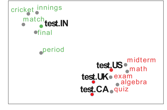
Figure 1: The latent semantic space captured by our method (geodist) reveals geographic variation between language speakers. In the majority of the English speaking world (e.g. US, UK, and Canada) a test is primarily used to refer to an exam, while in India a test indicates a lengthy cricket match which is played over five consecutive days.

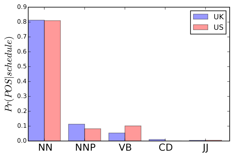
(a) Part of Speech distribution for schedule (Syntactic)

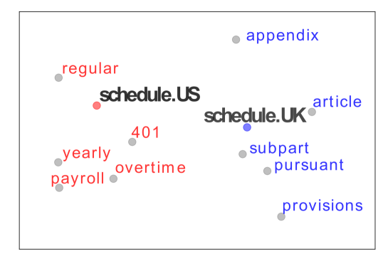
(b) Latent semantic space captured by geodist method.

Figure 2: The word schedule differs in its semantic usage between US and UK English which geodist (see Figure 2(b)) detects. While schedule in the USA refers to a “scheduling time”, in the UK schedule also has the meaning of an “addendum to a text”. However the Syntactic method (see Figure 2(a)) does not detect this semantic change since schedule is dominantly used as a noun (NN) in both UK and the USA.

Detecting and analyzing regional variation in language is central to the field of socio-variational linguistics and dialectology (eg. [40, 25, 31, 41]). Since online content is an agglomeration of material originating from all over the world, language on the Internet demonstrates geographic variation. The abundance of geo-tagged online text enables a study of geographic linguistic variation at scales that are unattainable using classical methods like surveys and questionnaires.

Characterizing and detecting such variation is challenging since it takes different forms: lexical, syntactic and semantic. Most existing work has focused on detecting lexical variation prevalent in geographic regions [4, 13, 15, 16]. However, regional linguistic variation is not limited to lexical variation.

In this paper we address this gap. Our method, geodist, is the first computational approach for tracking and detecting statistically significant linguistic shifts of words across geographical regions. geodist detects syntactic and semantic variation in word usage across regions, in addition to purely lexical differences. geodist builds on recently introduced neural language models that learn word representations (word embeddings), extending them to capture region-specific semantics. Since observed regional variation could be due to chance, geodist explicitly introduces a null model to ensure detection of only statistically significant differences between regions.

Figure 1 presents a visualization of the semantic variation captured by geodist for the word test between the United States, the United Kingdoms, Canada, and India. In the majority of English speaking countries, test almost always means an exam, but in India (where cricket is a popular sport) test almost always refers to a lengthy form of cricket match. One might argue that simple baseline methods like (analyzing part of speech) might be sufficient to identify regional variation. However because these methods capture different modalities, they detect different types of changes as we illustrate in Figure 2.

We use our method in two novel ways. First, we evaluate our methods on several large datasets at multiple geographic resolutions. We investigate linguistic variation across Twitter at multiple scales: (a) between four English speaking countries and (b) between fifty states in USA. We also investigate regional variation in the Google Books Ngram Corpus data. Our methods detect a variety of changes including regional dialectical variations, region specific usages, words incorporated due to code mixing and differing semantics.

Second, we apply our method to analyze distances between language dialects. In order to do this, we propose a measure of semantic distance between languages. Our analysis of British and American English over a period of $100$ years reveals that semantic variation between these dialects is shrinking potentially due to cultural mixing and globalization (see Figure 3).

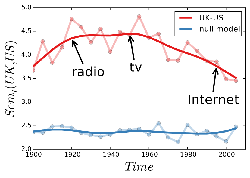
Figure 3: Semantic Distance between UK English and US English at different time periods from 1900-2005. The two countries are becoming closer to one another driven by globalization and invention of mass communication technologies like radio, television, and the Internet.

Specifically, our contributions are as follows:

• Models and Methods: We present our new method geodist which extends recently proposed neural language models to capture semantic differences between regions (Section 3.2). geodist is a new statistical method that explicitly incorporates a null model to ascertain statistical significance of observed semantic changes.

• Multi-Resolution Analysis: We apply our method on multiple domains (Books and Tweets) across geographic scales (States and Countries). Our analysis of these large corpora (containing billions of words) reveals interesting facets of language change at multiple scales of geographic resolution – from neighboring states to distant continents (Section 5).

• Semantic Distance: We propose a new measure of semantic distance between languages which we use to characterize distances between various dialects of English and analyze their convergent and divergent patterns over time (Section 6).

2 Problem Definition

We seek to quantify shift in word meaning (usage) across different geographic regions. Specifically, we are given a corpus $\mathcal{C}$ that spans $R$ regions where $\mathcal{C}_{r}$ corresponds to the corpus specific to region $r$. We denote the vocabulary of the corpus by $\mathcal{V}$. We want to detect words in $\mathcal{V}$ that have region specific semantics (not including trivial instances of words exclusively used in one region). For each region $r$, we capture statistical properties of a word $w$’s usage in that region. Given a pair of regions $(r_{i},r_{j})$, we then reduce the problem of detecting words that are used differently across these regions to an outlier detection problem using the statistical properties captured.

In summary, we answer the following questions:

1. In which regions does the word usage drastically differ from other regions?

2. How statistically significant is the difference observed across regions?

3. Given two regions, how close are their corresponding dialects semantically?

3 Methods

In this section we discuss methods to model regional word usage.

3.1 Baseline Methods

Frequency Method.

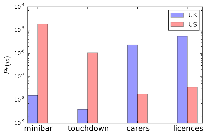
Figure 4: Frequency usage of different words in English UK and English US. Note that touchdown, an American football term is much more frequent in the US than in UK. Words like carers and licences are used more in the UK than in the US. carers are known as caregivers in the US and licences is spelled as licenses in the US.

One standard method to detect which words vary across geographical regions is to track their frequency of usage. Formally, we track the change in probability of a word across regions as described in [24]. To characterize the difference in frequency usage of $w$ between a region pair $(r_{i},r_{j})$, we compute the ratio $\textsc{Score}(w)=\frac{P_{r_{i}}(w)}{P_{r_{j}}(w)}$ where $P_{r_{i}}(w)$ is the probability of $w$ occurring in region $r_{i}$. An example of the information we capture by tracking word frequencies over regions is shown in Figure 4. Observe that touchdown (an American football term) is used much more frequently in the US than in UK. While this naive method is easy to implement and identifies words which differ in their usage patterns, one limitation is an overemphasis on rare words. Furthermore frequency based methods overlook the fact that word usage or meaning changes are not exclusively associated with a change in frequency.

Syntactic Method. A method to capture syntactic variation in word usage through time was proposed by [24]. Along similar lines, we can capture regional syntactic variation of words. The word lift is a striking example of such variation: In the US, lift is dominantly used as a verb (in the sense: “to lift an object”), whereas in the UK lift also refers to an elevator, thus predominantly used as a common noun. Given a word $w$ and a pair of regions $(r_{i},r_{j})$ we adapt the method outlined in [24] and compute the Jennsen-Shannon Divergence between the part of speech distributions for word $w$ corresponding to the regions.

Figure 5 shows the part of speech distribution for a few words that differ in syntactic usage between the US and UK. In the US, remit is used primarily as a verb (as in “to remit a payment”). However in the UK, remit can refer “to an area of activity over which a particular person or group has authority, control or influence” (used as “A remit to report on medical services”). The word curb is used mostly as a noun (as ”I should put a curb on my drinking habits.”) in the UK but it is used dominantly as a verb in the US (as in “We must curb the rebellion.”).

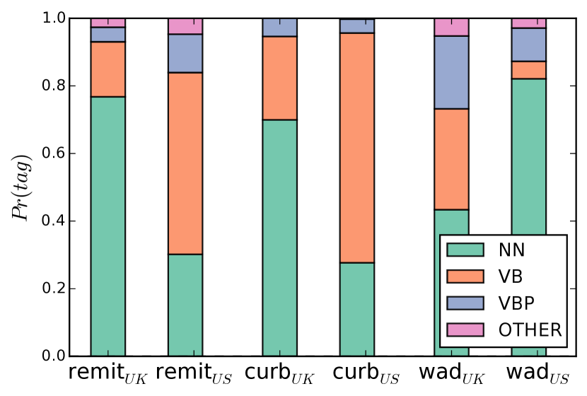
Figure 5: Part of speech tag probability distribution of the words which differ in syntactic usage between UK and US. Observe that remit is predominantly used a verb (VB) in the US but as a common noun (NN) in the UK.

Whereas the Syntactic method captures a deeper variation than the frequency methods, it is important to observe that semantic changes in word usage are not limited to syntactic variation as we illustrated before in Figure 2.

3.2 Distributional Method: geodist

As we noted in the previous section, linguistic variation is not restricted only to syntactic variation. In order to detect subtle semantic changes, we need to infer cues based on the contextual usage of a word. To do so, we use distributional methods which learn a latent semantic space that maps each word $w\in\mathcal{V}$ to a continuous vector space $\mathbb{R}^{d}$.

We differentiate ourselves from the closest related work to our method [5], by explicitly accounting for random variation between regions, and proposing a method to detect statistically significant changes.

Learning region specific word embeddings

Given a corpus $\mathcal{C}$ with $R$ regions, we seek to learn a region specific word embedding $\phi_{r}:\mathcal{V},\mathcal{C}_{r}\mapsto\mathbb{R}^{d}$ using a neural language model. For each word $w\in\mathcal{V}$ the neural language model learns:

1. A global embedding $\delta_{\text{MAIN}}(w)$ for the word ignoring all region specific cues.

2. A differential embedding $\delta_{r}(w)$ that encodes differences from the global embedding specific to region $r$.

The region specific embedding $\phi_{r}(w)$ is computed as: $\phi_{r}(w)=\delta_{\text{MAIN}}(w)+\delta_{r}(w)$. Before training, the global word embeddings are randomly initialized while the differential word embeddings are initialized to $\mathbf{0}$. During each training step, the model is presented with a set of words $w$ and the region $r$ they are drawn from. Given a word $w_{i}$, the context words are the words appearing to the left or right of $w_{i}$ within a window of size $m$. We define the set of active regions $\mathcal{A}=\{r,\text{MAIN}\}$ where MAIN is a placeholder location corresponding to the global embedding and is always included in the set of active regions. The training objective then is to maximize the probability of words appearing in the context of word $w_{i}$ conditioned on the active set of regions $\mathcal{A}$. Specifically, we model the probability of a context word $w_{j}$ given $w_{i}$ as:

$$\Pr(w_{j}\mid w_{i}) =\frac{\exp{(\mathbf{w}_{j}^{T}\mathbf{w}_{i})}}{\sum\limits_{w_{k}\in\mathcal{V}}\exp{(\mathbf{w}_{k}^{T}\mathbf{w}_{i})}}$$ (1)

where $\mathbf{w}_{i}$ is defined as $\mathbf{w}_{i}=\sum\limits_{a\in\mathcal{A}}\delta_{a}(w_{i})$.

During training, we iterate over each word occurrence in $\mathcal{C}$ to minimize the negative log-likelihood of the context words. Our objective function $J$ is thus given by:

$$J =\sum_{w_{i}\in\mathcal{C}}\sum_{\begin{subarray}{c}j=i-m\\ j!=i\end{subarray}}^{i+m}-\log\Pr(w_{j}\mid\mathbf{w}_{i})$$ (2)

When $|\mathcal{V}|$ is large, it is computationally expensive to compute the normalization factor in Equation 1 exactly. Therefore, we approximate this probability by using hierarchical soft-max [34, 32] which reduces the cost of computing the normalization factor from $\mathcal{O}(|\mathcal{V}|)$ to $\mathcal{O}(\log|\mathcal{V}|)$. We optimize the model parameters using stochastic gradient descent [8], as $\phi_{t}(w_{i})=\phi_{t}(w_{i})-\alpha\times\frac{\partial{J}}{\partial\phi_{t}(w_{i})}$ where $\alpha$ is the learning rate. We calculate the derivatives using the back-propagation algorithm [38]. We set $\alpha=0.025$, context window size $m$ to $10$ and size of the word embedding $d$ to be $200$ unless stated otherwise.

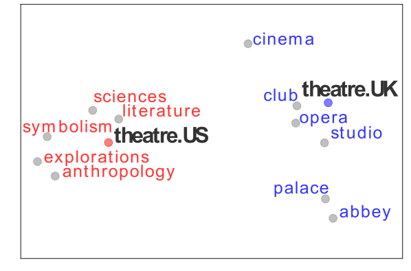
Figure 6: Semantic field of theatre as captured by geodist method between the UK and US. theatre is a field of study in the US while in the UK it primarily associated with opera or a club.

Distance Computation between regional embeddings

After learning word embeddings for each word $w\in{\mathcal{V}}$, we then compute the distance of a word between any two regions $(r_{i},r_{j})$ as $\textsc{Score}(w)=\textsc{CosineDistance}(\phi_{r_{i}}(w),\phi_{r_{j}}(w))$ where $\textsc{CosineDistance}(u,v)$ is defined by $1-\frac{u^{T}v}{\lVert u\rVert_{2}\lVert v\rVert_{2}}$.

Figure 6 illustrates the information captured by our geodist method as a two dimensional projection of the latent semantic space learned, for the word theatre. In the US, the British spelling theatre is typically used only to refer to the performing arts. Observe how the word theatre in the US is close to other subjects of study: sciences, literature, anthropology, but theatre as used in UK is close to places showcasing performances (like opera, studio, etc). We emphasize that these regional differences detected by geodist are inherently semantic, the result of a level of language understanding unattainable by methods which focus solely on lexical variation [17].

3.3 Statistical Significance of Changes

In this section, we outline our method to quantify whether an observed change given by $\textsc{Score}(w)$ is significant. When one is operating on an entire population (or in the absence of stochastic processes), one fairly standard method to identify outliers is the $Z$-value test [1] (obtained by standardizing the raw scores) and marking samples whose $Z$-value exceeds a threshold $\beta$ (typically set to the $95$th percentile) as outliers.

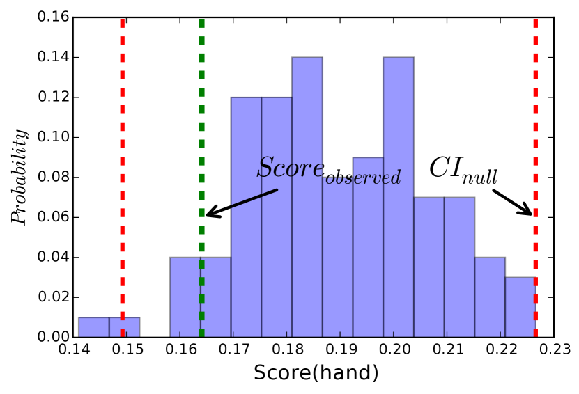
(a) Observed score for hand

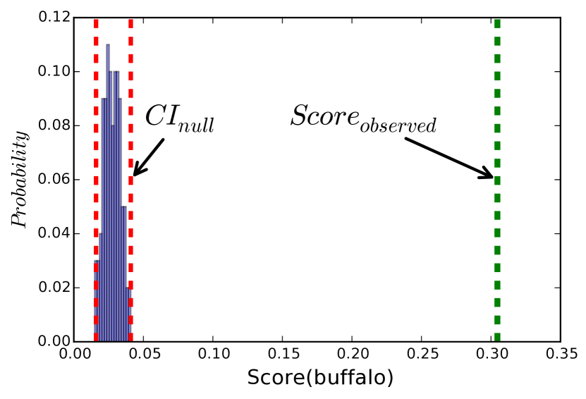
(b) Observed score for buffalo

Figure 7: The observed scores computed by geodist (in ) for buffalo and hand when analyzing regional differences between New York and USA overall. The histogram shows the distribution of scores under the null model. The $98\%$ confidence intervals of the score under null model are shown in . The observed score for hand lies well within the confidence interval and hence is not a statistically significant change. In contrast, the score for buffalo is far outside the confidence interval for the null distribution indicating a statistically significant change.

However since in our method, $\textsc{Score}(w)$ could vary due random stochastic processes (even possibly pure chance), whether an observed score is significant or not depends on two factors: (a) the magnitude of the observed score (effect size) and (b) probability of obtaining a score more extreme than the observed score, even in the absence of a true effect.

Specifically, given a word $w$ with a score $E(w)=\textsc{Score}(w)$ between regions $(r_{i},r_{j})$ we ask the question: “What is the chance of observing $E(w)$ or a more extreme value assuming the absence of an effect?”

First our method explicitly models the scenario when there is no effect, which we term as the null model. Next we characterize the distribution of scores under the null model. Our method then compares the observed score with this distribution of scores to ascertain the significance of the observed score. The details of our method are described in Algorithm 1 and below.

We simulate the null model by observing that under the null model, the labels of the text are exchangeable. Therefore, we generate a corpus $C^{\prime}$ by a random assignment of the labels (regions) of the given corpus $C$. We then learn a model using $C^{\prime}$ and estimate $\textsc{Score}(w)$ under this model. By repeating this procedure $B$ times we estimate the distribution of scores for each word under the null model (Lines 4 to 13).

After we estimate the distribution of scores we then compute the $100\alpha\%$ confidence interval on $\textsc{Score}(w)$ under the null model. Thus for each word $w$, we specify two measures: (a) observed effect size and (b) $100\alpha\%$ confidence interval (we typically set $\alpha=0.95$) corresponding to the null distribution (Lines 20-21). When the observed effect is not contained in the confidence interval obtained for the null distribution, the effect is statistically significant at the $1-\alpha$ significance level.

Even though $p$-values have been traditionally used to report significance, recently researchers have argued against their use as $p$-values themselves do not indicate what the observed effect size was and hence even very small effects can be deemed statistically significant [39, 14]. In contrast, reporting effect sizes and confidence intervals enables us to factor in the magnitude of effect size while interpreting significance. In a nutshell therefore, we deem a change observed for $w$ as statistically significant when:

1. The effect size exceeds a threshold $\beta$ which ensures the effect size is large enough. One typically standardizes the effect size and typically sets $\beta$ to the $95$th percentile (which is usually around $3$).

2. It is rare to observe this effect as a result of pure chance. This is captured by our comparison to the null model and the confidence intervals computed.

Figure 7 illustrates this for two words: hand and buffalo. Observe that for hand, the observed score is smaller than the higher confidence interval, indicating that hand has not changed significantly. In contrast buffalo which is used differently in New York (since buffalo refers to a place in New York) has a score well above the higher confidence interval under the null model.

Algorithm 1 ScoreSignificance ($C$, $B$, $\alpha$)

1:$C$: Corpus of text with $R$ regions, $B$: Number of bootstrap samples, $\alpha$: Confidence Interval threshold

2:$E$: Computed effect sizes for each word $w$, CI: Computed confidence intervals for each word $w$

3:// Estimate the NULL distribution.

4:$\textsc{BS}\leftarrow\emptyset$ {Corpora from the NULL Distribution}. $\textsc{NULLSCORES}(w)$ {Store the scores for $w$ under null model.}

5:repeat

6:   Permute the labels assigned to text of $C$ uniformly at random to obtain corpus $C^{\prime}$

7:   $\textsc{BS}\leftarrow\textsc{BS}\cup C^{\prime}$

8:   Learn a model $N$ using $C^{\prime}$ as the text.

9:   for $w\in\mathcal{V}$ do

10:      Compute $\textsc{Score}(w)$ using $N$.

11:      Append $\textsc{Score}(w)$ to $\textsc{NULLSCORES}(w)$

12:   end for

13:until $|\textsc{BS}|$ = $B$

14:// Estimate the actual observed effect and compute confidence intervals.

15:Learn a model $M$ using $C$ as the text.

16:for $w\in\mathcal{V}$ do

17:   Compute $\textsc{Score}(w)$ using $M$.

18:   $E(w)\leftarrow\textsc{Score}(w)$

19:   Sort the scores in $\textsc{NULLSCORES}(w)$.

20:   $\textsc{HCI}(w)$ $\leftarrow$ $100\alpha$ percentile in $\textsc{NULLSCORES}(w)$

21:   $\textsc{LCI}(w)\leftarrow 100(1-\alpha)$ percentile in $\textsc{NULLSCORES}(w)$

22:   $\textsc{CI}(w)$ $\leftarrow$ $(\textsc{LCI}(w),\textsc{HCI}(w))$

23:end for

24:return $E,\textsc{CI}$

As we will also see in Section 5, the incorporation of the null model and obtaining confidence estimates enables our method to efficaciously tease out effects arising due to random chance from statistically significant effects.

4 Datasets

Here we outline the details of two online datasets that we consider - Tweets from various geographic locations on Twitter and Google Books Ngram Corpus.

The Google Books Ngram Corpus

The Google Books Ngram Corpus corpus [27] contains frequencies of short phrases of text (ngrams) which were taken from books spanning eight languages over five centuries. While these ngrams vary in size from $1-5$, we use the $5$-grams in our experiments. Specifically we use the Google Books Ngram Corpus corpora for American English and British English and use a random sample of $30$ million ngrams for our experiments. Here, we show a sample of 5-grams along with their region:

•  drive a coach and horses (UK)
•  years as a football coach (US)

We obtained the POS Distribution of each word in the above corpora using Google Syntactic Ngrams[18, 26].

	Word	US/UK $\Delta$	Explanation
Books	zucchini	$2.3$	“zucchinis” are known as “courgettes” in UK
	touchdown	$2.4$	“touchdown” is a term in American football
	bartender	$2.5$	“bartender” is a very recent addition to the pub language in UK.
	Word	US/UK $\Delta$	Explanation
Tweets	freshman	$2.7$	“freshman” are referred to as “freshers” in the UK
	hmu	$2.5$	hit me up a slang which is popular in USA
		US/AU $\Delta$
	maccas	$-3.3$	McDonald’s in Australia is called maccas
	wickets	$-2.9$	wickets is a term in cricket, a popular game in Australia
	heaps	$-2.7$	Australian colloquial for “alot”

Table 1: Examples of words detected by the Frequency method on Google Book NGrams and Twitter. ($\Delta$ is difference in log probabilities between countries). A positive value indicates the word is more probable in the US than the other region. A negative value indicates the word is more probable in the other region than the US.

	Word	JS	US Usage	UK Usage
Books	remit	$0.173$	remit the loan	The jury investigated issues within its remit (an assigned area).
	oracle	$0.149$	Oracle the company	a person who is omniscient
	wad	$0.143$	a wad of cotton	Wad the paper towel and throw it! (used as “to compress”)
Tweets	sort	$0.224$	He’s not a bad sort	sort it out
	lift	$0.220$	lift the bag	I am stuck in the lift (elevator)
	ring	$0.200$	ring on my finger	give him a ring (call)
	cracking	$0.181$	The ice is cracking	The girl is cracking (beautiful)
	cuddle	$0.148$	Let her cuddle the baby (verb)	Come here and give me a cuddle (noun)
	dear	$0.137$	dear relatives	Something is dear (expensive)
			US Usage	AU Usage
	kisses	$0.320$	hugs and kisses (as a noun)	He kisses them (verb)
	claim	$0.109$	He made an insurance claim (noun)	I claim … (almost always used as a verb)

Table 2: Examples of words detected by the Syntactic method on Google Book NGrams and Twitter. (JS is Jennsen Shannon Divergence)

Word	Effect Size	CI(Null)	US Usage	UK Usage
theatre	0.6067	(0.004,0.007)	great love for the theatre	in a large theatre
schedule	0.5153	(0.032,0.050)	back to your regular schedule	a schedule to the agreement
forms	0.595	(0.015, 0.026)	out the application forms	range of literary forms (styles)
extract	0.400	(0.023, 0.045)	vanilla and almond extract	extract from a sermon
leisure	0.535	(0.012, 0.024)	culture and leisure (a topic)	as a leisure activity
extensive	0.487	(0.015, 0.027)	view our extensive catalog list	possessed an extensive knowledge (as in impressive)
store	0.423	(0.02, 0.04)	trips to the grocery store	store of gold (used as a container)
facility	0.378	(0.035, 0.055)	mental health,term care facility	set up a manufacturing facility (a unit)

(a) Google Book NGrams: Differences between English usage in the United States and United Kingdoms

Word	Effect Size	CI(Null)	US Usage	IN Usage
high	0.820	(0.02,0.03)	I am in high school	by pass the high way (as a road)
hum	0.740	(0.03, 0.04)	more than hum and talk	hum busy hain (Hinglish)
main	0.691	(0.048, 0.074)	your main attraction	main cool hoon (I am cool)
ring	0.718	(0.054, 0.093)	My belly piercing ring	on the ring road (a circular road)
test	0.572	(0.03, 0.061)	I failed the test	We won the test
stand	0.589	(0.046, 0.07)	I can’t stand stupid people	Wait at the bus stand

(b) Twitter: Differences between English usage in the United States and India

Table 3: Examples of statistically significant geographic variation of language detected by our method, geodist, between English usage in the United States and English usage in the United Kingdoms (a) and India (b). (CI - the $98\%$ Confidence Intervals under the null model)

Twitter Data

This dataset consists of a sample of Tweets spanning 24 months starting from September 2011 to October 2013. Each Tweet includes the Tweet ID, Tweet and the geo-location if available. We partition these tweets by their location in two ways:

1. States in the USA: We consider Tweets originating in the United States and group the Tweets by the state in the United States they originated from. The joint corpus consists of $7$ million Tweets.

2. Countries: We consider $11$ million Tweets originating from USA, UK, India (IN) and Australia (AU) and partition the Tweets among these four countries.

Some sample Tweet text is shown below:

•  Someone come to golden with us! (CA)
•  Taking the subway with the kids ...(NY)

In order to obtain part of speech tags, for the tweets we use the TweetNLP POS Tagger[36].

5 Results and Analysis

In this section, we apply our methods to various data sets described above to identify words that are used differently across various geographic regions. We describe the results of our experiments below.

5.1 Geographical Variation Analysis

Table 1 shows words which are detected by the Frequency method. Note that zucchini is used rarely in the UK because a zucchini is referred to as a courgette in the UK. Yet another example is the word freshman which refers to a student in their first year at college in the US. However in the UK a freshman is known as a fresher. The Frequency method also detects terms that are specific to regional cultures like touchdown, an American football term and hence used very frequently in the US.

As we noted in Section 4, the Syntactic method detects words which differ in their syntactic roles. Table 2 shows words like lift, cuddle which are used as verbs in the US but predominantly as nouns in the UK. In particular lift in the UK also refers to an elevator. While in the USA, the word cracking is typically used as a verb (as in “the ice is cracking”), in the UK cracking is also used as an adjective and means “stunningly beautiful”. The Frequency method in contrast would not be able to detect such syntactic variation since it focuses only on usage counts and not on syntax.

In Tables 3(a) and 3(b) we show several words identified by our geodist method. While theatre refers primarily to a building (where events are held) in the UK, in the US theatre also refers primarily to the study of the performing arts. The word extract is yet another example: extract in the US refers to food extracts but is used primarily as a verb in the UK. While in the US, the word test almost always refers to an exam, in India test has an additional meaning of a cricket match that is typically played over five days. An example usage of this meaning is “We are going to see the test match between India and Australia” or the “The test was drawn.”. We reiterate here that the geodist method picks up on finer distributional cues that the Syntactic or the Frequency method cannot detect. To illustrate this, observe that theatre is still used predominantly as a noun in both UK and the USA, but they differ in semantics which the Syntactic method fails to detect.

Word	Distances
	Naive Distances	nullmodel	geodist(Our Method)
buffalo
twins
space
golden
hand

Table 4: Sample set of words which differ in meaning (semantics) in different states of the USA. Note how incorporating the null model highlights only statistically significant changes. Observe how our method geodist correctly detects no change in hand.

Another clear pattern that emerges are “code-mixed words”, which are regional language words that are incorporated into the variant of English (yet still retaining the meaning in the regional language). Examples of such words include main and hum which in India also mean “I” and “We” respectively in addition to their standard meanings. In Indian English, one can use main as “the main job is done” as well as “main free at noon. what about you?”. In the second sentence main refers to “I” and means “I am free at noon. what about you?”.

Furthermore, we demonstrate that our method is capable of detecting changes in word meaning (usage) at finer scales (within states in a country). Table 4 shows a sample of the words in states of the USA which differ in semantic usage markedly from their overall semantics globally across the country.

Note that the usage of buffalo significantly differs in New York as compared to the rest of the USA. buffalo typically would refer to an animal in the rest of USA, but it refers to a place named Buffalo in New York. The word queens is yet another example where people in New York almost always refer to it as a place.

Other clear trends evident are words that are typically associated with states. Examples of such words include golden, space and twins. The word golden in California almost always refers to The golden gate bridge and space in Washington refers to The space needle. While twins in the rest of the country is dominantly associated with twin babies (or twin brothers), in the state of Minnesota, twins also refers to the state’s baseball team Minnesota Twins.

Table 4 also illustrates the significance of incorporating the null model to detect which changes are significant. Observe how incorporating the null model renders several observed changes as being not significant thus highlighting statistically significant changes. Without incorporating the null model, one would erroneously conclude that hand has different semantic usage in several states. However on incorporating the null model, we notice that these are very likely due to random chance thus enabling us to reject this as signifying a true change.

These examples demonstrate the capability of our method to detect wide variety of variation across different scales of geography spanning regional differences to code-mixed words.

6 Semantic Distance

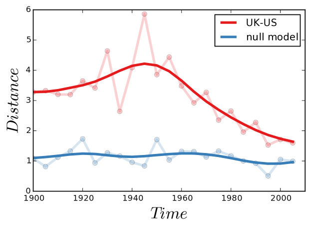
Figure 8: Usage of acts in UK converges to the usage in US over time.

In this section we investigate the following question: Are British and American English converging or diverging over time semantically?

In order to measure semantic distance between languages through time, we propose a measure of semantic distance between two variants of the language at a given point $t$. Specifically, at a given time $t$, we are given a corpus $\mathcal{C}$ and a pair of regions $(r_{i},r_{j})$. Using our method (see Section 3.2) we compute the standardized distance $Z_{t}(w)$ for each word $w$ between the regions at time point $t$. Then, we construct the intersection of the set of words $\mathcal{W}$ that have been deemed to have changed significantly at each time point $t$. We do this so that (a) we focus on only the words that were significantly different between the language dialects at time point $t$ and (b) the words identified as different are stable across time, allowing us to track the usage of the same set of divergent words over time. Our measure of the semantic distance between the two language dialects at time $t$ is then $Sem_{t}(r_{i},r_{j})=\frac{1}{|\mathcal{W}|}\sum_{w\in\mathcal{W}}Z_{t}(w)$, the mean of the distances of words in $\mathcal{W}$.

In our experiment, we considered the Google Books Ngram Corpus for UK English and US English within a time span of $1900-2005$ using a window of $5$ years. We computed the semantic distance between these dialects as described above, which we present in Figure 3. We clearly observe a trend showing both British and American English are converging. Figure 8 shows one such word acts, where the usage in the UK starts converging to the usage in the US. Before the 1950’s, acts in British English was primarily used as a legal term (with ordinances, enactments, laws etc). American English on the other hand used acts to refer to actions (as in acts of vandalism, acts of sabotage). However in the $1960$’s British English started adopting the American usage.

We hypothesize that this effect is observed due to globalization (the invention of radio, tv and the Internet), but leave a rigorous investigation of this phenomenon to future work.

While our measure of semantic distance between languages does not capture lexical variation, introduction of new words etc, our work opens the door for future research to design better metrics for measuring semantic distances while also accounting for other forms of variation.

7 Related Work

Most of the related work can be organized into two areas: (a) Socio-variational linguistics (b) Word embeddings

Socio-variational linguistics

A large body of work studies how language varies according to geography and time [15, 17, 4, 5, 23, 24, 22, 19].

While previous work like [20, 7, 23, 22, 9] focus on temporal analysis of language variation, our work centers on methods to detect and analyze linguistic variation according to geography. A majority of these works also either restrict themselves to two time periods or do not outline methods to detect when changes are significant. Recently [24] proposed methods to detect statistically significant linguistic change over time that hinge on timeseries analysis. Since their methods explicitly model word evolution as a time series, their methods cannot be trivially applied to detect geographical variation.

Several works on geographic variation [4, 15, 35, 13] focus on lexical variation. Bamman and others [4] study lexical variation in social media like Twitter based on gender identity. Eisenstein et al. [15] describe a latent variable model to capture geographic lexical variation. Eisenstein et al. [16] outline a model to capture diffusion of lexical variation in social media. Different from these studies, our work seeks to identify semantic changes in word meaning (usage) not limited to lexical variation. The work that is most closely related to ours is that of Bamman, Dyer, and Smith [5]. They propose a method to obtain geographically situated word embeddings and evaluate them on a semantic similarity task that seeks to identify words accounting for geographical location. Their evaluation typically focuses on named entities that are specific to geographic regions. Our work differs in several aspects: Unlike their work which does not explicitly seek to identify which words vary in semantics across regions, we propose methods to detect and identify which words vary across regions. While our work builds on their work to learn region specific word embeddings, we differentiate our work by proposing an appropriate null model, quantifying the change and assessing its significance. Furthermore our work is unique in the fact that we evaluate our method comprehensively on multiple web-scale datasets at different scales (both at a country level and state level).

Measures of semantic distance have been developed for units of language (words, concepts etc) which [33] provide an excellent survey. Cooper [12] study the problem of measuring semantic distance between languages, by attempting to capture the relative difficulty of translating various pairs of languages using bi-lingual dictionaries. Different from their work, we measure semantic distance between language dialects in an unsupervised manner (using word embeddings) and also analyze convergence patterns of language dialects over time.

Word Embeddings

The concept of using distributed representations to learn a mapping from symbolic data to continuous space dates back to Hinton [21]. In a landmark paper, Bengio et al. [6] proposed a neural language model to learn word embeddings and demonstrated that they outperform traditional n-gram based models. Mikolov et al. [29] proposed Skipgram models for learning word embeddings and demonstrated that they capture fine grained structures and linguistic regularities [28, 30]. Also [37] induce language networks over word embeddings to reveal rich but varied community structure. Finally these embeddings have been demonstrated to be useful features for several NLP tasks [11, 3, 2, 10].

8 Conclusions

In this work, we proposed a new method to detect linguistic change across geographic regions. Our method explicitly accounts for random variation, quantifying not only the change but also its significance. This allows for more precise detection than previous methods.

We comprehensively evaluate our method on large datasets at different levels of granularity – from states in a country to countries spread across continents. Our methods are capable of detecting a rich set of changes attributed to word semantics, syntax, and code-mixing. Using our method, we are able to characterize the semantic distances between dialectical variants over time. Specifically, we are able to observe the semantic convergence between British and American English over time, potentially an effect of globalization. This promising (although preliminary) result points to exciting research directions for future work.

References

- Aggarwal [2013] Aggarwal, C. C. 2013. Outlier analysis. Springer Science & Business Media.
- Al-Rfou et al. [2015] Al-Rfou, R.; Kulkarni, V.; Perozzi, B.; and Skiena, S. 2015. Polyglot-ner: Massive multilingual named entity recognition. In SDM.
- Al-Rfou, Perozzi, and Skiena [2013] Al-Rfou, R.; Perozzi, B.; and Skiena, S. 2013. Polyglot: Distributed word representations for multilingual nlp. In Proceedings of the Seventeenth Conference on Computational Natural Language Learning.
- Bamman and others [2014] Bamman, D., et al. 2014. Gender identity and lexical variation in social media. Journal of Sociolinguistics.
- Bamman, Dyer, and Smith [2014] Bamman, D.; Dyer, C.; and Smith, N. A. 2014. Distributed representations of geographically situated language. Proceedings of the 52nd Annual Meeting of the Association for Computational Linguistics (Volume 2: Short Papers) 828–834.
- Bengio et al. [2006] Bengio, Y.; Schwenk, H.; Senecal, J.-S.; Morin, F.; and Gauvain, J.-L. 2006. Neural probabilistic language models. In Innovations in Machine Learning.
- Berners-Lee et al. [2001] Berners-Lee, T.; Hendler, J.; Lassila, O.; et al. 2001. The Semantic Web. Scientific American.
- Bottou [1991] Bottou, L. 1991. Stochastic gradient learning in neural networks. In Proceedings of Neuro-Nîmes 91.
- Brigadir, Greene, and Cunningham [2015] Brigadir, I.; Greene, D.; and Cunningham, P. 2015. Analyzing discourse communities with distributional semantic models. In ACM Web Science 2015 Conference. ACM.
- Chen et al. [2013] Chen, Y.; Perozzi, B.; Al-Rfou, R.; and Skiena, S. 2013. The expressive power of word embeddings. arXiv preprint arXiv:1301.3226.
- Collobert et al. [2011] Collobert, R.; Weston, J.; Bottou, L.; Karlen, M.; Kavukcuoglu, K.; and Kuksa, P. 2011. Natural language processing (almost) from scratch. JMLR.
- Cooper [2008] Cooper, M. C. 2008. Measuring the semantic distance between languages from a statistical analysis of bilingual dictionaries*. Journal of Quantitative Linguistics.
- Doyle [2014] Doyle, G. 2014. Mapping dialectal variation by querying social media. In EACL.
- du Prel et al. [2009] du Prel, J.-B.; Hommel, G.; Röhrig, B.; and Blettner, M. 2009. Confidence interval or p-value?: part 4 of a series on evaluation of scientific publications. Deutsches Ärzteblatt International.
- Eisenstein et al. [2010] Eisenstein, J.; O’Connor, B.; Smith, N. A.; and Xing, E. P. 2010. A latent variable model for geographic lexical variation. In EMNLP.
- Eisenstein et al. [2014] Eisenstein, J.; O’Connor, B.; Smith, N. A.; and Xing, E. P. 2014. Diffusion of lexical change in social media. PLoS ONE.
- Eisenstein, Smith, and others [2011] Eisenstein, J.; Smith, N. A.; et al. 2011. Discovering sociolinguistic associations with structured sparsity. In In ACL-HLT.
- Goldberg and Orwant [2013] Goldberg, Y., and Orwant, J. 2013. A dataset of syntactic-ngrams over time from a very large corpus of english books. In *SEM.
- Gonçalves and Sánchez [2014] Gonçalves, B., and Sánchez, D. 2014. Crowdsourcing dialect characterization through twitter.
- Gulordava and Baroni [2011] Gulordava, K., and Baroni, M. 2011. A distributional similarity approach to the detection of semantic change in the google books ngram corpus. In GEMS.
- Hinton [1986] Hinton, G. E. 1986. Learning distributed representations of concepts. In Proceedings of the eighth annual conference of the cognitive science society.
- Kenter et al. [2015] Kenter, T.; Wevers, M.; Huijnen, P.; et al. 2015. Ad hoc monitoring of vocabulary shifts over time. In CIKM. ACM.
- Kim et al. [2014] Kim, Y.; Chiu, Y.-I.; Hanaki, K.; Hegde, D.; and Petrov, S. 2014. Temporal analysis of language through neural language models. In ACL.
- Kulkarni et al. [2015] Kulkarni, V.; Al-Rfou, R.; Perozzi, B.; and Skiena, S. 2015. Statistically significant detection of linguistic change. In WWW.
- Labov [1980] Labov, W. 1980. Locating language in time and space / edited by William Labov. Academic Press New York.
- Lin et al. [2012] Lin, Y.; Michel, J.-B.; Aiden, E. L.; et al. 2012. Syntactic annotations for the google books ngram corpus. In Proceedings of the ACL 2012 system demonstrations.
- Michel and others [2011] Michel, J.-B., et al. 2011. Quantitative analysis of culture using millions of digitized books. Science 331(6014):176–182.
- Mikolov and others [2013] Mikolov, T., et al. 2013. Linguistic regularities in continuous space word representations. In Proceedings of NAACL-HLT.
- Mikolov et al. [2013a] Mikolov, T.; Chen, K.; Corrado, G.; and Dean, J. 2013a. Efficient estimation of word representations in vector space. arXiv preprint arXiv:1301.3781.
- Mikolov et al. [2013b] Mikolov, T.; Sutskever, I.; Chen, K.; Corrado, G. S.; and Dean, J. 2013b. Distributed representations of words and phrases and their compositionality. In NIPS.
- Milroy [1992] Milroy, J. 1992. Linguistic variation and change: on the historical sociolinguistics of English. B. Blackwell.
- Mnih and Hinton [2009] Mnih, A., and Hinton, G. E. 2009. A scalable hierarchical distributed language model. NIPS.
- Mohammad and Hirst [2012] Mohammad, S. M., and Hirst, G. 2012. Distributional measures of semantic distance: A survey. arXiv preprint arXiv:1203.1858.
- Morin and Bengio [2005] Morin, F., and Bengio, Y. 2005. Hierarchical probabilistic neural network language model. In Proceedings of the international workshop on artificial intelligence and statistics.
- O’Connor et al. [2010] O’Connor, B.; Eisenstein, J.; Xing, E. P.; and Smith, N. A. 2010. Discovering demographic language variation. In Proc. of NIPS Workshop on Machine Learning for Social Computing.
- Owoputi, O’Connor, and others [2013] Owoputi, O.; O’Connor, B.; et al. 2013. Improved part-of-speech tagging for online conversational text with word clusters. Association for Computational Linguistics.
- Perozzi, Al-Rfou, and others [2014] Perozzi, B.; Al-Rfou, R.; et al. 2014. Inducing language networks from continuous space word representations. In Complex Networks V.
- Rumelhart, Hinton, and Williams [2002] Rumelhart, D. E.; Hinton, G. E.; and Williams, R. J. 2002. Learning representations by back-propagating errors. Cognitive modeling 1:213.
- Sullivan and Feinn [2012] Sullivan, G. M., and Feinn, R. 2012. Using effect size-or why the p value is not enough. Journal of graduate medical education.
- Tagliamonte [2006] Tagliamonte, S. A. 2006. Analysing Sociolinguistic Variation. Cambridge University Press.
- Wolfram and Schilling-Estes [2005] Wolfram, W., and Schilling-Estes, N. 2005. American English: dialects and variation, volume 20. Wiley-Blackwell.