Models for generalized spherical and
related distributions

Abstract

A flexible model is developed for multivariate generalized spherical distributions, i.e. ones with level sets that are star shaped. To work in dimension above 2 requires tools from computational geometry and multivariate numerical integration. In order to simulate from these star shaped contours, an algorithm to simulate from general tessellations has been developed that has applications in other situations. These techniques are implemented in an R package gensphere.

1 Introduction

There is a need for tractable models for multivariate data with nonstandard dependence structures. Our motivation here was to be able to flexibly model distributions with star-shaped level sets. An R package gensphere has been developed that allows one to work with these classes of distributions: specifying flexible shapes for the level sets, computing densities, and simulating. A deliberate goal in this process is to have methods and programs that work in dimension $d\geq 2$, and this requires some methods from computational geometry. While the original intent focused on star-shaped regions, some of the tools developed here are useful for other problems, e.g. sampling from more general sets

Fernández et al. (1995) proposed defining multivariate distributions from a contour $\mathcal{C}$ (a simple closed curve/surface in ${\mathbb{R}}^{d}$) that is specified by a contour function $c:{\mathbb{S}}\to[0,\infty)$:

$$\mathcal{C}=\{c({\mathbf{s}}){\mathbf{s}}\,:\,{\mathbf{s}}\in{\mathbb{S}}\}.$$

Here ${\mathbb{S}}=\{{\mathbf{s}}\in{\mathbb{R}}^{d}:|{\mathbf{x}}|=1\}$ is the unit sphere, a $(d-1)$-dimensional surface. We assume that $c({\mathbf{s}})$ is a continuous function. Figure 1 shows a 2-dimensional example and Figure 4 shows a 3-dimensional example.

Let $g:[0,\infty)\to[0,\infty)$ be a nonnegative function and define

$$f({\mathbf{x}})=\begin{cases}g\left(\frac{|{\mathbf{x}}|}{c({\mathbf{x}}/|{\mathbf{x}}|)}\right)&|{\mathbf{x}}|>0\\ g(0)&|{\mathbf{x}}|=0\end{cases}$$ (1)

Under integrability conditions discussed below, this will give a probability density function on ${\mathbb{R}}^{d}$, and the level sets of such a distribution are scalar multiples of $\mathcal{C}$. Such distributions are also called homothetic. We will call $c(\cdot)$ the contour function and $g(\cdot)$ the radial function of the distribution.

Our approach differs a bit from Fernández et al. (1995) because we take the contour function $c(\cdot)$ as the basic object, whereas they use $v({\mathbf{x}}):=|{\mathbf{x}}|/c({\mathbf{x}}/|{\mathbf{x}}|)$ as the basic object. This object is well studied in convex analysis and functional analysis where it is called a gauge function or Minkowski functional. By construction, $v$ is homogeneous: $v(a{\mathbf{x}})=|a|v({\mathbf{x}})$. If $c({\mathbf{s}})=1$, then $\mathcal{C}$ is the unit sphere and $v({\mathbf{x}})=|{\mathbf{x}}|$, so the resulting classes of distributions are the spherical/isotropic distributions. If $v(\cdot)$ is convex, then $v(\cdot)$ is a norm on ${\mathbb{R}}^{d}$ and $\mathcal{C}$ is the unit ball in that norm, hence the name $v$-spherical distributions. When $v(\cdot)$ is not convex, e.g. an $\ell_{p}$ ball with $p<1$, $v({\mathbf{x}})$ does not give a norm, so $\mathcal{C}$ is not strictly speaking a unit ball, but we will still call the resulting distributions $v$-spherical.

The purpose of this paper is to describe a method of defining a flexible class of generalized spherical distributions in any dimension $d\geq 2$, and to describe an R package gensphere that implements this method. The package gives the ability to

1. define a flexible set of contours

2. carefully tessellate a contour

3. sample from a tessellation

4. use a contour and a radial function $g(\cdot)$ to define a generalized spherical distribution

5. compute the density $f(\cdot)$ given by (1)

6. approximately simulate from a distribution with density $f(\cdot)$.

The third step above also provides a way to simulate from paths and surfaces unrelated to generalized spherical laws.

Other references on generalized spherical laws are Arnold et al. (2008), Kamiya et al. (2008), Rattihalli and Basugade (2009), Rattihalli and Patil (2010), and Balkema and Nolde (2010). These papers develop the idea of generalized spherical distributions, but do not provide general purpose software for working with these distributions and don’t cover techniques for working with higher dimensional models.

2 Generalized spherical distributions

For (1) to be a proper density, it is required that (see Fernández et al. (1995), e.g.. (4) and (5))

$$k_{\mathcal{C}}^{-1}:=\int_{{\mathbb{S}}}c^{d}({\mathbf{s}})d{\mathbf{s}}\in(0,\infty)$$ (2)

and

$$\int_{0}^{\infty}r^{d-1}g(r)dr=k_{\mathcal{C}}.$$ (3)

We will assume $c(\cdot)$ is continuous on ${\mathbb{S}}$ and that $c({\mathbf{s}})\leq c_{0}$. This guarantees (2) is finite, though evaluating it may be difficult even when $d=2$, and especially when $d>2$.

2.1 Stochastic representation

Given any univariate density $h(\cdot)$ on the positive axis, the function $g(r)=k_{\mathcal{C}}r^{1-d}h(r)$ is a valid radial function. This is the approach we use in the rest of this paper and in the gensphere package. In this case the positive random variable $R$ with density $h(\cdot)$ gives a stochastic representation of the generalized spherical random vector:

$${\mathbf{X}}{\stackrel{{\scriptstyle d}}{{=}}}R{\mathbf{Z}},$$ (4)

where ${\mathbf{Z}}$ is uniformly distributed on the contour $\mathcal{C}$. This directly gives a way to simulate ${\mathbf{X}}$ if ${\mathbf{Z}}$ can be simulated. Balkema and Nolde (2010) give a related stochastic representation

$${\mathbf{X}}{\stackrel{{\scriptstyle d}}{{=}}}R^{*}{\mathbf{Z}}^{*},$$

where ${\mathbf{Z}}^{*}$ is uniformly distributed on the unit disk $\mathcal{D}=\{{\mathbf{x}}\in{\mathbb{R}}^{d}:v({\mathbf{x}})\leq 1\}$. An advantage of this is that it is straightforward, though possibly inefficient, to simulate from $\mathcal{D}$ by generating a uniform vector on a rectangle that contains the ball $\mathcal{D}$ and rejecting if $v({\mathbf{x}})>1$. We prefer to use (4) and describe below how to approximately sample from the contour $\mathcal{C}$.

2.2 Specification of a contour function

For modeling purposes, we want a flexible family of functions that can be used in a variety of problems. To be able to include the distributions discussed by the authors cited above, we allow contour functions of the form

$$c({\mathbf{s}})=\sum_{j=1}^{N_{1}}c_{j}r_{j}({\mathbf{s}})+\displaystyle{\frac{1}{\sum_{j=1}^{N_{2}}c^{*}_{j}r^{*}_{j}({\mathbf{s}})}},$$

where $c_{j}>0$, $c^{*}_{j}>0$, and $r_{j}(\cdot)$ and/or $r^{*}(\cdot)$ are one of the cases discussed below.

1. $r({\mathbf{s}})=1$, which makes $\mathcal{C}$ the Euclidean ball.

2. $r({\mathbf{s}})=c({\mathbf{s}}|\mbox{\boldmath$\mu$},\theta)$ is a cone with peak 1 at center $\mbox{\boldmath$\mu$}\in{\mathbb{S}}$ and height 0 at the base given by the circle $\{{\mathbf{x}}\in{\mathbb{S}}:\mbox{\boldmath$\mu$}\cdot{\mathbf{x}}=\cos\theta\}$. It is assumed that $|\theta|\leq\pi/2$.

3. $r({\mathbf{s}})=c({\mathbf{s}}|\mbox{\boldmath$\mu$},\sigma)=\exp(-t({\mathbf{s}})^{2}/(2\sigma^{2}))$ is a Gaussian bump centered at location $\mbox{\boldmath$\mu$}\in{\mathbb{S}}$ and “standard deviation” $\sigma>0$. Here $t({\mathbf{s}})$ is the distance between $\mu$ and the projection of ${\mathbf{s}}\in{\mathbb{S}}$ linearly onto the plane tangent to ${\mathbb{S}}$ at $\mu$.

4. $r^{*}({\mathbf{s}})=||{\mathbf{s}}||_{\ell^{p}({\mathbb{R}}^{d})}$, $p>0$.

5. $r^{*}({\mathbf{s}})=||A{\mathbf{s}}||_{\ell^{p}({\mathbb{R}}^{m})}$, $p>0$, $A$ an $(m\times d)$ matrix. This allows a generalized $p$-norm. If $A$ is $d\times d$ and orthogonal, then the resulting contour will be a rotation of the standard unit ball in $\ell^{p}$. If $A$ is $d\times d$ and not orthogonal, then the contour will be sheared. If $m>d$, it will give the $\ell^{p}$ norm on ${\mathbb{R}}^{m}$ of $A{\mathbf{s}}$.

6. $r^{*}({\mathbf{s}})=({\mathbf{s}}^{T}A{\mathbf{s}})^{1/2}$, where $A$ is a positive definite $(d\times d)$ matrix. Then the level curves of the distribution are ellipses.

Sums of the first three types allow us to describe star shaped contours, see Figure 1. Inverses of sums of the last two types allow us to consider contours that are familiar unit balls, or generalized unit balls, or sums of such shapes. An implementation of this construction is given in a new R package gensphere. The R statements used in this example are given in the Appendix.

It is relatively easy to add new types of terms to this list if other contours are of interest. However this set of basic shapes can model a wide range of shapes, including contours supported on a cone. Figure 3 shows nine examples. The top row shows $\ell_{p}$ balls with $p=1/2$, $p=1$, and $p=5$. The middle row starts with a contour made up of an $\ell_{p}$ ball with a $p=0.3$ and a copy of that rotated by $\pi/4$, the rotation done by using a generalized $\ell_{p}$ norm with $A$ a rotation matrix. The next two plots show generalized $\ell_{p}$ balls with $A=(1,1;1,-4;1,3;5,-3)$ and $p=1/2$ (middle) and $p=1.1$ (right). The last row shows contours supported on a cone. The left plot is the sum of three Gaussian bumps of type 3, each centered at $(\cos\theta,\sin\theta)$, $\theta=\pi/4,\pi/2,3\pi/2$ and $\sigma=0.3$. The middle plot has two type 2 cones, at angles $-\pi/6$ and $-\pi/3$ with $\sigma=0.4$. The last graph also has two cones, centered at $\pi/6$ and $\pi/3$, with $\sigma=0.25$. Any of the contours that have a corner or cusp on a ray will generate a density surface with a ridge along that ray. A more complicated three dimensional example with 11 terms in the definition of $c(\cdot)$ is given in Figure 4.

Figure 1: Constructing a 2-dimensional contour. The top left plot shows a base of type 1, a circle of radius 1. The top right shows the base with one Gaussian bump of type 3 in direction $(\sqrt{2}/2,\sqrt{2}/2)$, the bottom left shows the final contour with another Gaussian bump in direction (-1,0). The bottom right plot shows a sample of size $n=1000$ from this contour using the method described in Section 3.

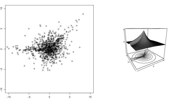
Figure 2: On the left is a sample from the generalized spherical distribution based on the contour in Figure 1 and a $\Gamma$(2,1) radial term. On the right, is a surface plot of the density $f(x,y)$.

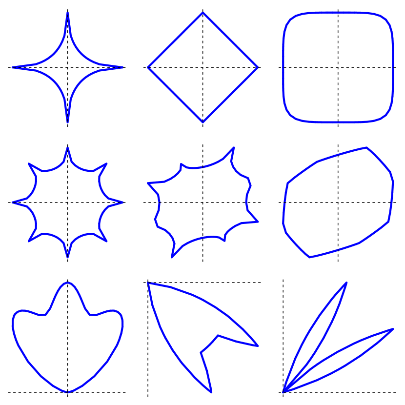
Figure 3: A selection of contours made from the different types of terms. See the text for a description.

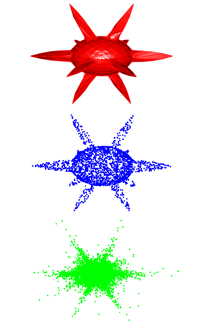
Figure 4: A 3D star-shaped region with one term of type 6 and 10 terms of type 2. The top plot shows the contour, the middle shows a sample of size 2500 from the contour, the bottom shows a sample of size 10000 from the generalized spherical distribution given by this contour and a $\Gamma(3,1)$ radial term $R$.

2.3 Choice of $R$

In general, $g(r)$ can be any nonnegative integrable function. In most applications one wants $0<g(0)<\infty$ and $g(r)$ decreasing for $r>0$. If $g(0)=0$, the density surface given by (1) will have a “well” at the origin; if $g(0)=+\infty$, then the density blows up at the origin. If $g(\cdot)$ oscillates, then the density surface will have radial “waves” emanating out from the origin. If $R$ has bounded support, then ${\mathbf{X}}$ will have bounded support. The radial decay of $R$ determines the decay of $f(\cdot)$ on ${\mathbb{R}}^{d}$.

The gamma distribution give a family of distributions that can by used to get generalized spherical distributions with light tails. If a $\Gamma(d,1)$ law is used for $R$, then $h(r)=\Gamma(d)^{-1}r^{d-1}\exp(-r)$, so $g(r)=k_{\mathcal{C}}r^{1-d}h(r)=(k_{\mathcal{C}}/\Gamma(d))\exp(-r)$, which is finite at the origin and monotonically decreasing. If one wants heavy tails for ${\mathbf{X}}$, then some possibilities for $R$ are Fréchet, Pareto and multivariate stable amplitude. (The latter is defined in Nolan (2013) by $R=|{\mathbf{Z}}|$, where ${\mathbf{Z}}$ is radially symmetric/isotropic $\alpha$-stable in $d$-dimensions. Numerical methods to calculate the density $h(r)$ of $R$ and simple ways to simulate are given in the reference.)

Figure 5 shows the effect that the choice of $R$ has. In all cases, the base contour is the unit ball in $\ell_{1}$, a diamond shape. At the upper left, $R$ is a uniform r.v. on (0,1). In this case, $g(0)=+\infty$ and the density has a spike at the origin and bounded support on the diamond. At the top right, $R\sim\Gamma(2,1)$, so $g(0)=1$ and the distribution has unbounded support with light tails. At the lower left, $R$ is the $\alpha=1$ stable amplitude in $d=2$ dimensions; here $g(0)$ is finite and the distribution has heavy tails. The bottom right plot is with $R\sim\Gamma(5,1)$, so $g(0)=0$ and the distribution has a well at the origin and unbounded support with light tails.

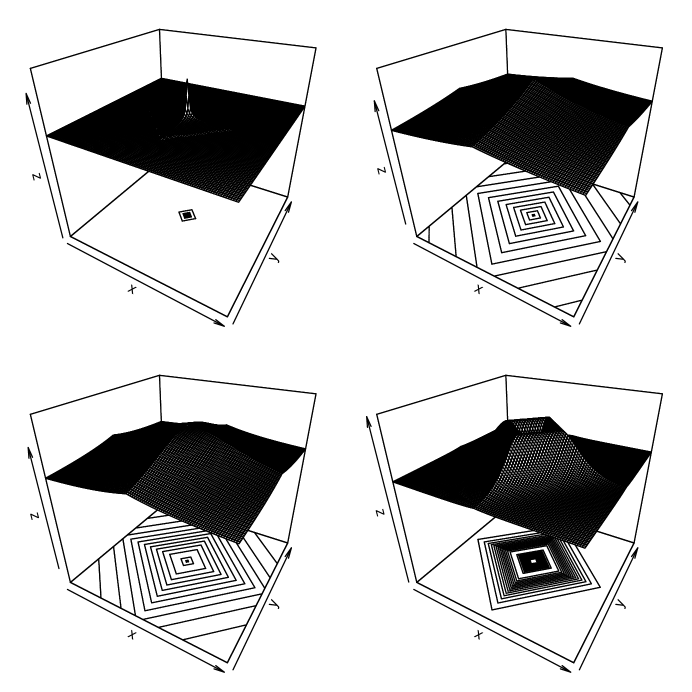
Figure 5: Density surface for generalized spherical distributions with the same diamond shape and different radial term $R$ as specified in the text.

3 Contours: tessellating, integrating and simulating

A large part of the technical complexity of working with generalized spherical laws is in evaluating the norming constant $k_{\mathcal{C}}$ in (2) and simulating from the contour $\mathcal{C}$. The gensphere package uses two other recent R packages for these problems: SphericalCubature Nolan (2015b) and mvmesh Nolan (2015a).

SphericalCubature numerically integrates a function on a $d$-dimensional sphere. Given a tessellation of the sphere in ${\mathbb{R}}^{d}$, it uses adaptive integration to integrate over the $(d-1)$-dimensional surface to evaluate $k_{\mathcal{C}}$. If the integrand function is smooth and the tessellation is reasonable, then the numerical integration is accurate in modest dimensions, say $d=2,3,4,5,6$. However, when the integrand function has abrupt changes, numerical techniques can miss parts of the integral. This is even a problem in dimension 2, where the integration is a one dimensional problem. One way to deal with this is to work with tessellations that focus on the places where the integrand is not smooth. In complete generality, this is hard to do. However, in evaluating integral (2) for one of the contours described above, we have an implicit description of where the contour changes abruptly.

The mvmesh package is used to define multivariate meshes, e.g. a collection of vertices and grouping information that specify a list of simplices that approximate a contour. The first place where mvmesh is used in gensphere is to give a grid on the sphere ${\mathbb{S}}$ in $d$-dimensions, e.g. the top left plot in Figure 1. mvmesh has a function UnitSphere that computes an approximately equal surface area approximation to a hypersphere in dimension $d$. It takes a parameter $k$ to say how many recursive subdivisions are used in each octant. Then this tessellation is refined by adding points on the to the sphere centered on the places where the contour has bumps, e.g. the cone and Gaussian bumps (type 2 and 3). Then the new points are combined with the original tessellation of the sphere to get a refined tessellation of the sphere that includes these key points.

It is at this point that the SphericalCubature package is used to evaluate the integral (3). In addition to the estimate of the integral, we use an option in the adaptive integration routine to return the partition used in the multivariate cubature, along with the estimated integral over each simplex. The reasoning is that the integration routine is subdividing regions where the integrand is changing quickly to get a better estimate of the integrand. This subdivision should make the tessellation more closely approximate the contour. We now have the final tessellation of the unit sphere, an estimate of the integral (2) over each of the simplices, and an estimate of the norming constant, e.g. sum of these just mentioned values.

Now the tessellation of the contour is defined by deforming the tessellation on the sphere to the contour: each partition point ${\mathbf{s}}\in{\mathbb{S}}$ gets mapped to $c({\mathbf{s}}){\mathbf{s}}$ on the contour. The grouping information from the spherical tessellation is inherited by the contour tessellation. This tessellation is returned as an S3 object of class “mvmesh”. This object contains the vertices, the grouping information, and a list of all the simplices $S_{1},S_{2},\ldots,S_{k}$ in the tessellation. One advantage of this is that the plot method the mvmesh package can plot the contours in 2 and 3 dimensions. This process of refining the tessellation has two purposes: (a) get a more accurate estimate of the norming constant by focusing the numerical integration routine on regions where the integrand changes rapidly and (b) get a more accurate tessellation of the contour. Each step of this process can add more simplices, with the goal of capturing key features of the contour. For example, the contour in Figure 4 started with 512 simplices in the tessellation of the sphere in ${\mathbb{R}}^{3}$ with $k=3$, adding the points on the cone brought the number up to 888 simplices, and after the adaptive cubature routine subdivision there were 2284 simplices.

Exact simulation from a surface is a challenging problem and general methods are difficult to apply for complicated contours like our star shaped regions. We now describe an approximate method based on the above tessellation. Recall that the above process gives us a list of simplices $S_{1},\ldots,S_{k}$ and associated weights $w_{1},\ldots,w_{k}$ that are estimates of the integral on each simplex; $w_{j}$ is an estimate of the surface area of the contour approximated by simplex $S_{j}$.

The simulation routine is now straightforward:

1. select an index $j$ with probability proportional to $w_{j}$.

2. simulate a point ${\mathbf{u}}$ that is uniformly distributed on the unit simplex in $d$-dimensions. This is standard: simulate a Dirichlet distribution with parameter $\mbox{\boldmath$\alpha$}=(1,1,\ldots,1)$, e.g. let $E_{1},\ldots,E_{d}$ i.i.d. standard exponential random variates and set ${\mathbf{u}}=(E_{1},\ldots,E_{d})/\left(\sum_{i=1}^{d}E_{i}\right)$.

3. map the point ${\mathbf{u}}$ to the simplex $S_{j}$ using the coordinates of ${\mathbf{u}}$ as barycentric coordinates: ${\mathbf{Z}}={\mathbf{u}}^{T}S_{j}$.

4. simulate $R$ from the radial distribution with density $h(r)$.

5. return the value ${\mathbf{X}}=R{\mathbf{Z}}$.

This method works in any dimension and the first three steps is adaptable to a wide variety of shapes, more than just the contours described above. For the generalized spherical distributions the weights are proportional to surface area, e.g. the bottom right plot in Figure 1, but they can be assigned in any way. Figure 6 illustrates some examples with different shapes and where the weights are defined in different ways. In all cases the points ${\mathbf{Z}}$ are sampled from the simplex faces; too work well the tessellation should closely model the shape of the surface of interest.

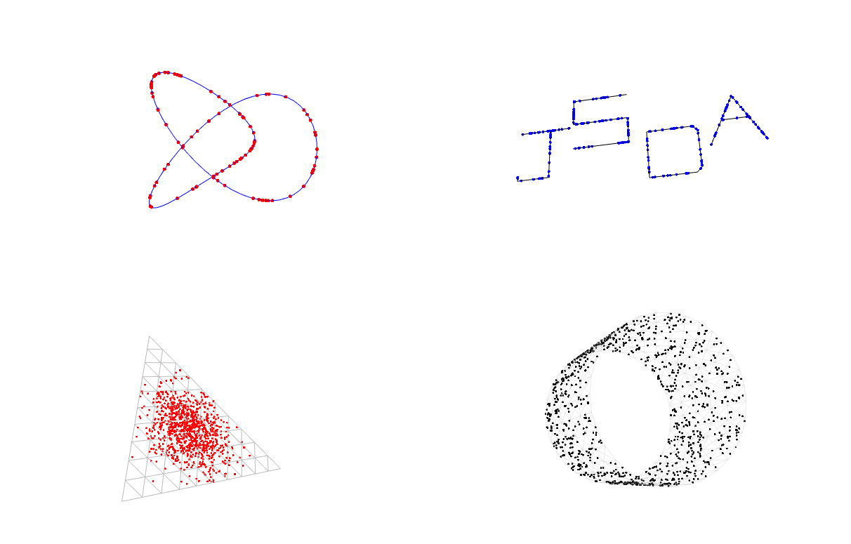
Figure 6: Simulation from general sets. Top left is a trefoil knot, the points are sampled uniformly. Top right has the letters JSDA embedded in ${\mathbb{R}}^{3}$ and points are sampled uniformly on them. Bottom left has points sampled on the unit simplex according to a density $\exp(-c|{\mathbf{x}}-(\frac{1}{3},\frac{1}{3},\frac{1}{3})|^{2})$. The last plot shows points sampled uniformly from a hollow tube.

The subdivision process, including the numerical cubature is the slowest part of the process. This is done in the R function cfunc.finish, which finishes the definition of a contour by performing these calculations and saving the results in an object of class “contour.function”. For the example in Figure 4, it can take several minutes to complete the construction. The simulation and density calculations are fast, taking only a few seconds. Producing the graphs can be slow; the top plot in Figure 4 with 2284 simplices took over 1/2 an hour to plot.

In contrast, once the tessellation is produced, density calculations and simulations are quite fast: to evaluate a density at 10000 points takes less than a second, and to simulate $n=10000$ random vectors takes less than a second in a bivariate example with two terms.

In principle, the methods described here work in any dimension; in practice the numerical challenges, particularly evaluating the integral in (2) and the time needed to work limit us as the dimension increases.

Appendix A Appendix

Here are the R statements used to produce Figures 1 and 2 from the R package gensphere.

# define a new contour function (cfunc)
cfunc <- cfunc.new(d=2)
cfunc <- cfunc.add.term( cfunc,"constant",k=1)
cfunc <- cfunc.add.term( cfunc,"proj.normal",
             k=c( 1, sqrt(2)/2, sqrt(2)/2, 0.1) )
cfunc <- cfunc.add.term( cfunc,"proj.normal",
             k=c( 1, -1,0, 0.1) )
cfunc <- cfunc.finish( cfunc, k=4 )

# define a generalized spherical distribution with the
# above contour and a gamma radial component
rradial <- function( n ) { rgamma( x, shape=2 ) }
dradial <- function( x ) { dgamma( x, shape=2 ) }
dist <- gensphere( cfunc, dradial, rradial, g0=1 )

# simulate from the generalized spherical distribution
x <- rgensphere( 1000, dist )

# compute the density
xx <- matrix(1:8,nrow=2)
dgensphere( xx, dist )

# simulate from the tessellation of the contour
x <- rtessellation( n=500, (cfunc$tessellation)$S,
     cfunc$tessellation.weights )

Appendix B Competing Interests

I confirm that I have read SpringerOpen’s guidance on competing interests and have no competing interests in the manuscript.

References

- Arnold et al. (2008) Arnold, B. C., E. Castillo, and J. M. Sarabia (2008). Multivariate distributions defined in terms of contours. Journal of Statistical Planning and Inference 138(12), 4158 – 4171.
- Balkema and Nolde (2010) Balkema, G. and N. Nolde (2010). Asymptotic independence for unimodal densities. Adv. in Appl. Probab. 42(2), 411–432.
- Fernández et al. (1995) Fernández, C., J. Osiewalski, and M. F. J. Steel (1995). Modeling and inference with -spherical distributions. Journal of the American Statistical Association 90(432), 1331–1340.
- Kamiya et al. (2008) Kamiya, H., A. Takemura, and S. Kuriki (2008). Star-shaped distributions and their generalizations. J. Statist. Plann. Inference 138(11), 3429–3447.
- Nolan (2013) Nolan, J. P. (2013). Multivariate elliptically contoured stable distributions: theory and estimation. Computational Statistics 28(5), 2067–2089.
- Nolan (2015a) Nolan, J. P. (2015a). mvmesh: Multivariate Meshes and Histograms in Arbitrary Dimensions. R package version 1.1, on CRAN.
- Nolan (2015b) Nolan, J. P. (2015b). SphericalCubature: Numerical Integration over Spheres and Balls in n-Dimensions; Multivariate Polar Coordinates. R package version 1.1, on CRAN.
- Rattihalli and Basugade (2009) Rattihalli, R. N. and A. B. Basugade (2009). Generation of densities using contour transformations. J. Indian Statist. Assoc. 47(1), 63–90.
- Rattihalli and Patil (2010) Rattihalli, R. N. and P. Y. Patil (2010). Generalized -spherical densities. Comm. Statist. Theory Methods 39(19), 3568–3583.