Classical Dynamical Gauge Fields in Optomechanics

Abstract

Artificial gauge fields for neutral particles such as photons, recently attracted a lot of attention in various fields ranging from photonic crystals to ultracold atoms in optical lattices to optomechanical arrays. Here we point out that, among all implementations of gauge fields, the optomechanical setting allows for the most natural extension where the gauge field becomes dynamical. The mechanical oscillation phases determine the effective artificial magnetic field for the photons, and once these phases are allowed to evolve, they respond to the flow of photons in the structure. We discuss a simple three-site model where we identify four different regimes of the gauge-field dynamics. Furthermore, we extend the discussion to a two-dimensional lattice. Our proposed scheme could for instance be implemented using optomechanical crystals.

I Introduction

Optomechanics describes the interaction of light and mechanical motion Aspelmeyer2014 . The prototypical optomechanical setting consists in a Fabry-Pérot cavity where one of the mirrors is free to oscillate. Due to the radiation pressure force the light inside the cavity interacts with the mirror’s motion. Tremendous experimental progress has been made during the last years to exploit this very elementary light-matter interaction, with achievements such as cooling a nanomechanical oscillator to its motional ground state Teufel2011 ; Chan2011a and position measurements below the standard quantum limit Teufel2009 , to name only a few examples. Mechanically and/or optically coupling several optomechanical systems leads to interesting new physics. For instance, setups consisting of only a few optical and mechanical modes allow for nonreciprocal devices for photons Manipatruni2009 ; Habraken2012 ; Hafezi2012 ; Wang2015 ; Ruesink2015 ; Fang2016 . Furthermore, one- or two-dimensional arrays of coupled optomechanical systems are promising candidate systems for studying many-body physics of photons or phonons Bhattacharya2008 ; Chang2011 ; Xuereb2012 ; Tomadin2012 ; Schmidt2012 ; Akram2012 ; Chen2012 ; Schmidt2015a ; Schmidt2015b ; Peano2014 . Most interestingly, optomechanical arrays are also a platform to create artificial gauge fields for photons Schmidt2015b and phonons Peano2014 . The optomechanical implementation complements other proposals for generating artificial gauge fields for photons Haldane2008 ; Wang2009 ; Koch2010 ; Umucallar2011 ; Hafezi2011 ; Fang2012b ; Hafezi2013 ; Rechtsman2013 ; Lu2014 ; Mittal2014 and ultracold atoms in optical lattices Jaksch2003 ; Sorensen2005 ; Lin2009 ; Aidelsburger2011 ; Aidelsburger2013 ; Jotzu2014 .

In this article, we study the most basic phonon-assisted photon tunneling process which is due to the optomechanical interaction. We show that an elementary optomechanical setting naturally gives rise to dynamical gauge fields. The key ingredient is a self-oscillating mechanical mode which connects two optical modes. Most importantly this brings an additional degree of freedom into play, viz. the mechanical oscillation phase. This mechanical oscillation phase is connected to an effective magnetic field seen by the photons and possesses its own dynamics.

During the last years, several proposal have been put forward dealing with the deliberate generation of dynamical gauge fields. Platforms based on ultracold atoms in optical lattices Osterloh2005 ; Ruseckas2005 ; Zohar2011 ; Hauke2012 ; Banerjee2012 ; Zohar2013 ; Edmonds2013 or superconducting circuits Marcos2013 ; Marcos2014 are discussed as promising systems which could serve as quantum simulators for dynamical gauge theories such as quantum electrodynamics and quantum chromodynamics Wiese2013 ; Zohar2015 . In most cases these proposals require a great deal of engineering, meaning carefully choosing a setting which yields the desired interactions between for instance superconducting qubits. Instead we concentrate on the intriguing optomechanical setting which gives rise to dynamical gauge fields in a very natural way. Particularly, in our scenario only basic phonon-assisted photon tunneling processes generated via the basic optomechanical interaction are needed. Besides the purpose of quantum simulation for dynamical gauge theories, the optomechanical setting opens up new directions dealing with nonlinear pattern formation of dynamical gauge fields in driven and dissipative systems Lauter2015 .

In the following, we investigate the evolution of the mechanical oscillation phases (the dynamical gauge field) in response to the light field dynamics, which is a unique feature of the optomechanical case. We consider a photonic lattice (representing the matter fields) and artificial gauge fields (phonons) which can be attributed to directed links between two sites of the photonic lattice. Such a system could for instance be implemented in optomechanical crystal structures Eichenfield2009 ; Safavi2010a ; Safavi2010b ; Gavartin2011 ; Chan2011a ; Safavi2014 or disk resonator arrays Zhang2015 .

II Generic Model for Dynamical Gauge Fields with Optomechanics

The crucial ingredient in our model is the phonon-assisted photon tunneling that can be generated by the optomechanical interaction: A photon $a$ hopping from site to site is accompanied by the coherent emission or absorption of a phonon $b$. This can be described by the Hamiltonian ($\hbar=1$)

$$H=\sum_{j}\nu_{j}^{\phantom{{\dagger}}}a_{j}^{{\dagger}}a_{j}^{\phantom{{\dagger}}}+\sum_{l}\omega_{l}^{\phantom{{\dagger}}}b_{l}^{{\dagger}}b_{l}^{\phantom{{\dagger}}}+\sum_{l}J_{l}^{\phantom{{\dagger}}}b_{l}^{\phantom{{\dagger}}}a_{l_{2}}^{{\dagger}}a_{l_{1}}^{\phantom{{\dagger}}}+{\rm{H.c.}}\,.$$ (1)

Here, $j$ denotes a lattice site, and $l=(l_{1},l_{2})$ is the index for a directed link from $l_{1}$ to $l_{2}$. A photon hopping in the direction of the link absorbs a phonon. Photons (phonons) have frequencies $\nu_{j}$ ($\omega_{l}$), and $J_{l}$ are the phonon-assisted photon tunneling amplitudes. We introduce the notation $b_{ij}=b_{ji}^{{\dagger}}$ and note that we use $b_{l}$ and $b_{l_{1}l_{2}}$ interchangeably. In Eq. (1) we made use of the rotating wave approximation which is valid for $\omega_{l}>\kappa,J_{l}$, where $\kappa$ is the photon decay rate. Non-reciprocity in photon transport can be engineered by coherent inelastic transitions induced by mechanical vibrations Schmidt2015b . However, in contrast to Ref. Schmidt2015b, we will treat the vibrations as dynamical degrees of freedom. In order to make the inelastic processes resonant, the nearest neighbor on-site photon frequencies have to differ by the corresponding link phonon frequency ($\omega_{ij}=\nu_{j}-\nu_{i}$) with the link direction from site $i$ to $j$. This leads to directed links. Generally speaking, a photon tunneling from a site with a low (high) on-site frequency to a site with a high (low) on-site frequency absorbs (emits) a phonon. We include photon losses at a rate $\kappa$ and account for driving by adding the term $H_{d}=\sum_{j}E_{j}\left(a_{j}e^{i\omega_{d}t}+a_{j}^{{\dagger}}e^{-i\omega_{d}t}\right)$ to Eq. (1), see A.

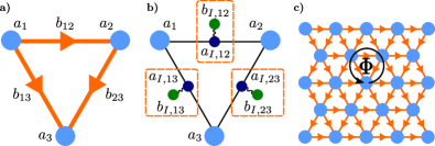
Figure 1: a) Effective model for a three-site optomechanical implementation of dynamical gauge fields for photons $a$ (light blue) coupling to phonons $b$ (orange). For the optical frequencies we choose $\nu_{1}<\nu_{2}<\nu_{3}$ leading to directed links, i.e., photons hopping in direction of the orange arrow absorb a phonon. b) Possible realization making use of the so-called “modulated link” scheme. Dark blue (green) dots depict intermediate optical (mechanical) modes which couple optomechanically to form an optomechanical cell (dashed box). c) Two-dimensional triangular lattice.

Our effective model, Fig. 1 a), can be realized in an optomechanical setting by building on the “modulated link” scheme that had been proposed to generate static artificial magnetic fields Schmidt2015b . In this scheme, the link between two optical modes $i$ and $j$ is realized with an intermediate optical mode $a_{I,l}$ which couples optomechanically to a mechanical mode $b_{I,l}$, forming a single optomechanical cell, cf. Fig. 1 b). In Ref. Schmidt2015b, the mechanical mode is externally driven into a large amplitude state $\langle{b_{I,l}(t)}\rangle=B_{I,l}e^{-i(\Omega_{I,l}t+\phi)}$ which leads to a modulation of the frequency of the intermediate optical mode $\omega_{I,j}(t)=\omega_{I,j}+2g_{0}B_{I,l}\cos(\Omega_{I,l}t+\phi)$. $g_{0}$ is the single-photon optomechanical coupling strength. We note that other microscopic implementations are possible. For example, one might have a mechanical mode that directly couples to the hopping between optical modes, as has been worked out in detail for optomechanical crystals Safavi2011 . This would be connected to the “wavelength conversion scheme” discussed in Ref. Schmidt2015b, .

In contrast to these two scenarios, we will assume that the mechanical oscillator undergoes self-sustained optomechanical oscillations Aspelmeyer2014 instead of being externally driven. Thus it behaves as a limit-cycle oscillator with a fixed amplitude $B$ and a free phase $\phi$. We will later show that the phase of the mechanical limit-cycle oscillator posses its own dynamics and that it will respond to the flow of photons in the system. This phase will then be directly linked to a dynamical gauge field. We want to stress that such mechanical self-sustained oscillations are a very generic feature of optomechnical systems. Therefore an optomechanical implementation of a dynamical gauge field requires less engineering than other proposals Osterloh2005 ; Ruseckas2005 ; Zohar2011 ; Hauke2012 ; Banerjee2012 ; Zohar2013 ; Edmonds2013 ; Marcos2013 ; Marcos2014 .

III Gauge Field Dynamics

Here we will focus on the classical dynamics of the model, i.e., the limit of large coherent photon and phonon amplitudes. This is the most relevant regime for most of the current optomechanical setups (due to the small single-photon coupling strength $g_{0}$) Aspelmeyer2014 . Thus, we decompose the expectation values of the photon and phonon operators into a classical amplitude and a phase, $a_{j}=A_{j}e^{i\theta_{j}}$ and $b_{ij}=B_{ij}e^{i\phi_{ij}}$. From the full quantum Heisenberg equations of motion for the effective Hamiltonian, the equations for the mechanical phases $\phi_{ij}$ become

$$\dot{\phi}_{ij} =-\omega_{ij}-\frac{J_{ij}}{B_{ij}}A_{i}A_{j}\cos(\phi_{ij}+\theta_{ij})\,,$$ (2)

while the optical amplitudes $A_{i}$ obey

$$\dot{A}_{i}=-\sum_{j\neq i}J_{ij}B_{ij}\sin(\phi_{ij}+\theta_{ij})A_{j}\,,$$ (3)

and the optical phases $\theta_{i}$ evolve according to

$$\dot{\theta}_{i}=-\nu_{i}-\sum_{j\neq i}J_{ij}B_{ij}\frac{A_{j}}{A_{i}}\cos(\phi_{ij}+\theta_{ij})\,.$$ (4)

We introduced $\theta_{jk}=\theta_{j}-\theta_{k}$ and used $\phi_{ij}=-\phi_{ji}$. Here and in the following we assume that the amplitudes of the limit-cycle oscillations are a constant of motion, i.e., $\dot{B}_{ij}=\dot{B}_{ji}=0$. This regime can be reached by working with self-induced optomechanical oscillators sufficiently above threshold Marquardt2006 . The initial phase of the self-oscillators would be random without extra precautions, but it can be set via an externally imposed mechanical drive, realized through an intensity-modulated light field.

In principle, the quantum regime of the present model could also be discussed, if the optomechanical coupling would be strong. The most straightforward extension to a quantum version can be realized considering that the mechanical oscillators on the links feature limit-cycles with quantum coherent phase dynamics. Another more demanding way towards dynamical gauge fields in the quantum regime with optomechanics would be in the spirit of Refs. Osterloh2005, ; Ruseckas2005, ; Zohar2011, ; Hauke2012, ; Banerjee2012, ; Zohar2013, ; Edmonds2013, ; Marcos2013, ; Marcos2014, . There, the link variable can be considered as a spin that flips each time an excitation hops between the corresponding sites. In the optomechanical case, this would require highly nonlinear mechanical oscillators that can be brought into the quantum regime such that they effectively act as a two-level system.

An important point we want to make at this stage is the invariance of the equations of motion under the following local $U(1)$ gauge transformation

$$\phi_{ij}^{\prime} =\phi_{ij}+\left(\chi_{j}-\chi_{i}\right)\,,$$ (5)

$$\theta_{i}^{\prime} =\theta_{i}+\chi_{i}\,,$$ (6)

meaning that the observed evolution of the light intensity will not change, independent of the choice of $\chi_{j}$. We assumed a static gauge choice $\chi$; otherwise Eqs. (5) and (6) would have to be supplemented by a change in frequencies: $\omega_{ij}^{\prime}=\omega_{ij}+\dot{\chi}_{i}-\dot{\chi}_{j}$ and $\nu_{i}^{\prime}=\nu_{i}-\dot{\chi}_{i}$.

Under which conditions does the gauge field display nontrivial dynamics? In Eqs. (2),  (3), and (4) we can rescale time by $JB$, where we assume link independent tunneling and mechanical amplitudes. Doing this, we observe that the entire dynamics only depends on the dimensionless ratio of $A/B$. Here, $A$ is proportional to the laser drive amplitude and corresponds to the optical amplitude at an arbitrary reference site in the lattice (globally lowering the optical amplitudes will also lower the optical amplitude at the reference site). For the limit $A/B\to 0$, we expect that the oscillation phases will not be affected by the hopping photons, rather only defining a static magnetic field pattern. This can be seen from Eq. (2): for $A/B\ll 1$ the second term, which provides the coupling to the hopping photons, can be neglected. However, if $A/B$ is large, we expect back-action of the hopping photons on the phonons leading to intriguing coupled dynamics of the gauge field.

IV Three-Site Model

First, we study the case of three sites. The resulting effective model for photons $a_{j}$ on sites $j\in\{1,2,3\}$ and phonons $b_{l}$ on links $l\in\{12,23,13\}$ is depicted in Fig. 1 a), where we define $a_{4}=a_{1}$. For definiteness, we will assume $\nu_{1}<\nu_{2}<\nu_{3}$. For three sites, the gauge freedom implies that only the gauge invariant flux

$$\Phi=\phi_{13}+\phi_{21}+\phi_{32}\,,$$ (7)

i.e., the sum of phases around the triangular plaquette, affects the dynamics of the photons. We want to mention that in the regime where the phonons are not influenced by the photons ($\Phi=\textrm{const.}$) the Hamiltonian for the three-site model can be diagonalized and the setup can act (for $\Phi=\pm\pi/2$) as a photon circulator Koch2010 , see also B.

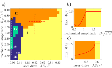
Figure 2: a) Dynamical regimes of the flux $\Phi$. Phase diagram as a function of mechanical amplitude and laser drive (which is resonant on site $1$, $\omega_{d}=\nu_{1}$) showing four regimes for the flux dynamics. In regimes I and II the flux $\Phi$ is stationary and tends to a value equal to $\pi/2$ or different from it, respectively. In regimes III and IV the flux $\Phi$ is dynamical and can either show a periodic oscillatory or chaotic behavior, respectively. b) and c) Cuts along the red dashed lines in a) across the phase transition from regime I to II.

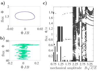
Figure 3: Examples of phase space trajectories $\Phi(t)-\dot{\Phi}(t)$ in region III and IV are shown in a) and b), respectively. c) Bifurcation diagram for the flux dynamics. We display the values of $\Phi(t)$ attained at the zero-crossings of $\dot{\Phi}(t)$. For the bifurcation diagram c) we used a higher resolution for values of $B\sqrt{J/E}$ than for the phase diagram in Fig. 2 a).

In the intriguing case where the photons interact with the phonons we discuss the driven and dissipative setting and furthermore choose equal tunneling amplitudes $J_{l}=J$ and mechanical amplitudes $B_{l}=B$. As an example we consider a resonant drive on site $j=1$. Without drive and dissipation the dynamics only depends on the ratio $A/B$. As a consequence, for the driven case, the four parameters involved $(E,\kappa,B,J)$, can be combined into just two dimensionless parameters, $B\sqrt{J/E}$ and $JE/\kappa^{2}$. The resulting “phase diagram” for the flux dynamics as a function of these two parameters is displayed in Fig. 2 a). It has been obtained from direct numerical simulations and reveals four distinct regimes. In regimes I and II the flux $\Phi(t)$ (after some transient behavior) approaches a stationary value of either $\Phi(t\to\infty)=\pi/2$ or different from it, respectively. In regimes III and IV, the flux $\Phi(t)$ is not stationary but even in the long-time limit shows a dynamical behavior. Most interestingly, the flux dynamics $\Phi(t)$ in these regimes can either show periodic or chaotic behavior, region III and IV in Fig. 2 a), respectively. Figures 2 b) and c) show cuts along the red dashed lines marked in the phase diagram, indicating a continuous phase transition from phase I to II. In Fig. 3 a) and b), we show two examples of the phase space $\Phi(t)-\dot{\Phi}(t)$ in regimes III and IV. Already at this level we can distinguish periodic [Fig. 3 a)] from chaotic [Fig. 3 b)] dynamics. A more involved characterization can be done using a bifurcation diagram. To this end, we show the value of $\Phi(t)$ evaluated at the zero crossings of $\dot{\Phi}(t)$, in the long-time limit, as a function the mechanical amplitude $B$ in Fig. 3 c). This bifurcation diagram allows us to distinguish the periodic from the chaotic flux dynamics within the whole phase diagram for $\Phi(t)$. In addition, we also checked whether the Fourier transform of the trajectories shows a clear peak or is flat, indicating periodic or chaotic behavior, respectively, see C.

In the regime of fast photons dynamics (compared to the phonon dynamics), we are able to apply a Born-Oppenheimer approximation and adiabatically eliminate the photons. To be more precise, we solve $da_{i}/dt=0$ where $\dot{a}_{j}=\left[-i(\nu_{j}-\omega_{d})-\frac{\kappa}{2}\right]a_{j}-iE_{j}-iJB\sum_{k\neq j}e^{-i\phi_{jk}}a_{k}$ and use this instantaneous solution to eliminate $a_{i}$ from the equations of motion for $\phi_{ij}$, see B. In the case of a resonant drive on site $j=1$, this approximation leads to the following equation of motion for the flux:

$$\dot{\Phi}=\frac{16E^{2}}{JB^{3}}\frac{(4+\frac{\kappa^{2}}{J^{2}B^{2}})\cos(\Phi)}{\frac{\kappa^{2}}{J^{2}B^{2}}[12+\frac{\kappa^{2}}{J^{2}B^{2}}]^{2}+[16\cos(\Phi)]^{2}}\,.$$ (8)

From Eq. (8) we find $\Phi(t\to\infty)=\pi/2$ which shows very good agreement with the exact numerical long-time dynamics in regime I. This approach fails in the other regimes since there we are not able to adiabatically eliminate the photons. We also want to mention that both $\Phi=+\pi/2$ and $\Phi=-\pi/2$ are fixed points of Eq. (8). It turns out that for a resonant drive on site $j=1$, $\Phi=-\pi/2$ is an unstable fixed point of Eq. (8). The asymmetry between $+\pi/2$ and $-\pi/2$ is due to the breaking of translational invariance, necessarily produced by the link directions. In contrast, a resonant drive on site $j=2\,(3)$ would have $\Phi=-\pi/2\,(+\pi/2)$ as a stable fixed point. From Eq. (8) we also can estimate the rate $\Gamma$ at which the flux $\Phi(t)$ settles into steady state. By linearizing around the fixed point we find $\Gamma=[16E^{2}(4+\xi)]/[JB^{3}\xi(12+\xi)^{2})]$ where $\xi=(\kappa/JB)^{2}$.

V Lattices

We extend the three-site model to two-dimensional lattices and illustrate the dynamical behaviour on a triangular lattice, cf. Fig. 1 c). Going from three sites to a lattice, a significant new feature comes into play: the artificial dynamical magnetic field produced by the phonons can now exert a Lorentz force that bends the path of any light-beam propagating in the array. Therefore, we end up with a dynamical interplay where the flow of the photons changes the spatial distribution of the magnetic flux density which then acts back on the dynamics of the light field. We choose a scenario with the link directions as depicted in Fig. 1 c). We note that this is not the only possible choice. In fact the intricate photon and phonon dynamics depends on the link pattern. We illustrate the nonlinear structure formation in this model for the case of having only a single site illuminated by a laser. In Fig. 4 a) we show the temporal evolution of the light intensity (top row) as well as the magnetic field (bottom row) on the lattice. At first the photons experience a static magnetic field which is set by the initial phases of the mechanical oscillations (here chosen such that the initial flux is $\Phi=\pi/2$) and start to move along the edge. Due to the back-action of the photons (which primarily move along the edge) on the phonons, the flux per plaquette changes. This in turn leads to a reconfiguration of the magnetic field which in this scenario forces the photons to reverse their direction of motion. Here, the system does not reach a steady state even in the long-time limit. Even though the photons live only for a short time $1/\kappa$ before escaping the structure, the system develops a spatial “memory” in the form of the mechanical oscillation phases, where previous photons leave their imprint.

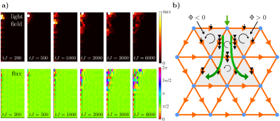
Figure 4: a) Evolution of the light field on a lattice with a dynamical gauge field of vibrational origin. Light intensity $A_{i,j}^{2}$ on each site (top row) and flux $\Phi$ per plaquette (bottom row) at different times. The resonant drive is on the site on the corner and the initial flux per plaquette is $\Phi=\pi/2$. No steady state of either photons or phonons is reached. We chose $B\sqrt{J/E}=3.16$, $JE/\kappa^{2}=10$ and have $1/\kappa=1/J$. The simulations were carried out on a $21\times 21$ triangular lattice, where only the left half is shown. b) Schematics of the flux and light field dynamics for the very first moments of the time evolution. Initially $\Phi=0$ for every plaquette and a single optical site is driven (green arrow). A finite optical amplitude on neighboring sites changes the mechanical phases, indicated by the black arrows. The number of arrowheads indicates the magnitude of decrease. The link directions lead to a negative (positive) flux through the left (right) plaquette next to the illuminated site. The direction of light transport is indicated by the green arrows.

For an intuitive description of the dynamics we assume zero initial flux per plaquette $\Phi=0$, a large optical damping $\kappa$ compared to the tunneling $J$, and a drive on one optical site on the top edge of the lattice. For this scenario, we show in Fig. 4 b) a schematics of the flux and light field dynamics and focus on the fluxes through the gray plaquettes for the very first moments of time evolution. As soon as the optical amplitudes of two neighboring optical sites is nonzero, the mechanical oscillation phase on the corresponding link will change, cf. Eq. (2). More precisely, the phases on the links decrease, indicated by the black arrows where the number of arrowheads indicate the magnitude of decrease. However, from the way these phases enter the photon dynamics, one can deduce that each phase contributes to the flux inside a plaquette with a positive sign only if the respective link is traversed in the positive direction when going around the plaquette counterclockwise. This leads to the signs shown in the figure. The light propagation due to the magnetic field is indicated by the green arrows. It is worth mentioning that even in the long-time limit the mechanical oscillation phases continue drifting because even an arbitrarily small but finite optical amplitude on neighboring sites is enough to change the phases, albeit very slowly. With such a scenario one could imagine to engineer a desired magnetic field pattern by means of an optical drive.

VI Disorder

In general, disorder effects in optomechanical arrays have been recognized as an important issue, especially in systems where the coupling between optical modes cannot be larger than the GHz-scale mechanical frequencies, as is the case both in the present system as well as, e.g., in our proposal for topologically protected transport in optomechanics Peano2014 . The transport of photons and phonons in disordered optomechanical arrays in the regime of Anderson localization has recently been analyzed in some detail by our group Roque2016 . To avoid such effects, the disorder needs to be suppressed down to a level of the photon tunneling or less in order to obtain localization lengths that are so large that they do not matter any more (larger than either the system size or the photon decay length). However, recently significant progress has been made regarding the fabrication of optomechanical crystal arrays, representing the most promising integrated nanoscale platform for these types of experiments. Specifically, it has been possible to reduce the disorder by a factor of about $100$ using novel postprocessing techniques, which brings it down to a scale where photon localization lengths become very large. These techniques have been exploited recently in an experiment on optomechanical non-reciprocity with two coupled modes Fang2016 which is quite close in spirit to the setup we would require here.

VII Conclusion

We have shown that dynamical gauge fields in optomechanical arrays arise quite naturally. The evolving mechanical oscillation phases, which respond to the flow of the photons, represent a dynamical gauge field for the latter. Already the three-site model shows intriguing dynamics which leads to a rather complex phase diagram for the flux dynamics. With experiments pushing towards multi-mode optomechanical setups, the three-site model seems feasible to be realized in the near future and would pave the way for further studies of dynamical gauge fields in optomechanical arrays. Collective behavior such as synchronization and pattern formation of mechanical limit-cycle oscillators have recently been studied in optomechanical arrays Heinrich2011 ; Ludwig2013 ; Lauter2015 . In this spirit, further studies on gauge field dynamics in optomechanics could address questions on synchronization and dynamical pattern formation of the magnetic field.

We acknowledge helpful discussions with Roland Lauter, and thank Vittorio Peano and Talitha Weiss for a careful reading of the manuscript. This work was financially supported by the Marie Curie ITN cQOM and the ERC OPTOMECH.

Appendix A The Three-Site Model: Including drive and dissipation

Since the photons eventually decay, we add photon loss and drive to the system. This is best done starting with the Hamiltonian (16) and adding a driving term $H_{d}=\sum_{j\in\{1,2,3\}}E_{j}\left(a_{j}e^{i\omega_{d}t}+a_{j}^{{\dagger}}e^{-i\omega_{d}t}\right)$. Going into a frame rotating with the driving frequency $\omega_{d}$, we obtain

$$H =\sum_{j\in\{1,2,3\}}(\nu_{j}^{\phantom{{\dagger}}}-\omega_{d})a_{j}^{{\dagger}}a_{j}^{\phantom{{\dagger}}}+\sum_{j\in\{1,2,3\}}E_{j}\left(a_{j}+a_{j}^{{\dagger}}\right)+\sum_{l\in\{12,23,13\}}\omega_{l}^{\phantom{{\dagger}}}b_{l}^{{\dagger}}b_{l}^{\phantom{{\dagger}}}$$ (9)

$$+J_{12}B_{12}\left(e^{-i\phi_{12}}a_{1}^{{\dagger}}a_{2}^{\phantom{{\dagger}}}+{\rm{H.c.}}\right)+J_{23}B_{23}\left(e^{-i\phi_{23}}a_{2}^{{\dagger}}a_{3}^{\phantom{{\dagger}}}+{\rm{H.c.}}\right)+J_{13}B_{13}\left(e^{i\phi_{13}}a_{3}^{{\dagger}}a_{1}^{\phantom{{\dagger}}}+{\rm{H.c.}}\right)\,.$$

Including dissipation of the photons at a rate $\kappa$ and neglecting effects due to quantum noise, the equations of motion for the photons become $d\vec{a}/dt=-iM\vec{a}-i\vec{E}$ with

$$\vec{a} =(a_{1},a_{2},a_{3})^{\textrm{T}}\,,$$ (10)

$$\vec{E} =(E_{1},E_{2},E_{3})^{\textrm{T}}\,,$$ (11)

$$M =\left(\begin{array}[]{ccc}(\nu_{1}-\omega_{d})-i\frac{\kappa}{2}&J_{12}B_{12}e^{-i\phi_{12}}&J_{13}B_{13}e^{-i\phi_{13}}\\ J_{12}B_{12}e^{i\phi_{12}}&(\nu_{2}-\omega_{d})-i\frac{\kappa}{2}&J_{23}B_{23}e^{-i\phi_{23}}\\ J_{13}B_{13}e^{i\phi_{13}}&J_{23}B_{23}e^{i\phi_{23}}&(\nu_{3}-\omega_{d})-i\frac{\kappa}{2}\end{array}\right)\,.$$ (15)

The equations of motion for the phases $\phi_{ij}$ are unchanged. In Fig. 5 we show the optical amplitude $\left|\langle a_{j}\rangle\right|^{2}=\left|A_{j}\right|^{2}$ as a function of the flux $\Phi$ and the drive frequency $\omega_{d}$. Figure 5 almost resembles the eigenfrequencies $\Omega_{k}$ in Fig. 6 c) which we obtained from diagonalizing the Hamiltonian.

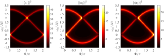
Figure 5: Left: $\left|A_{1}\right|^{2}$. Middle: $\left|A_{2}\right|^{2}$. Right: $\left|A_{3}\right|^{2}$. Here we only drive site $j=1$, i.e., $E_{1}=E,E_{2}=E_{3}=0$ and choose $JE/\kappa^{2}=0.025$, and $B\sqrt{J/E}=31.6$.

Appendix B The Three-Site Model: Diagonalization

Here, we give some further details on the three-site model given by Eq. (1) which in its explicit form reads

$$H =\sum_{j\in\{1,2,3\}}\nu_{j}^{\phantom{{\dagger}}}a_{j}^{{\dagger}}a_{j}^{\phantom{{\dagger}}}+\sum_{l\in\{12,23,13\}}\omega_{l}^{\phantom{{\dagger}}}b_{l}^{{\dagger}}b_{l}^{\phantom{{\dagger}}}+J_{12}\left(b_{12}^{\phantom{{\dagger}}}a_{2}^{{\dagger}}a_{1}^{\phantom{{\dagger}}}+{\rm{H.c.}}\right)+J_{23}\left(b_{23}^{\phantom{{\dagger}}}a_{3}^{{\dagger}}a_{2}^{\phantom{{\dagger}}}+{\rm{H.c.}}\right)+J_{13}\left(b_{13}^{{\dagger}}a_{1}^{{\dagger}}a_{3}^{\phantom{{\dagger}}}+{\rm{H.c.}}\right)\,.$$ (16)

The equations of motion are obtained straight forwardly by using Heisenberg’s equation of motion. The mechanical phases $\phi_{ij}$ evolve according to

$$\dot{\phi}_{12} =-\omega_{12}-\frac{J_{12}}{B_{12}}A_{1}A_{2}\cos(\phi_{12}+\theta_{12})\,,$$ (17)

$$\dot{\phi}_{23} =-\omega_{23}-\frac{J_{23}}{B_{23}}A_{2}A_{3}\cos(\phi_{23}+\theta_{23})\,,$$ (18)

$$\dot{\phi}_{13} =-\omega_{13}-\frac{J_{13}}{B_{13}}A_{1}A_{3}\cos(\phi_{13}+\theta_{13})\,.$$ (19)

The optical amplitudes $A_{j}$ obey the following equations of motion

$$\dot{A}_{1}= -J_{12}B_{12}\sin(\phi_{12}+\theta_{12})A_{2}-J_{13}B_{13}\sin(\phi_{13}+\theta_{13})A_{3}\,,$$ (20)

$$\dot{A}_{2}= +J_{12}B_{12}\sin(\phi_{12}+\theta_{12})A_{1}-J_{23}B_{23}\sin(\phi_{23}+\theta_{23})A_{3}\,,$$ (21)

$$\dot{A}_{3}= +J_{13}B_{13}\sin(\phi_{13}+\theta_{13})A_{1}+J_{23}B_{23}\sin(\phi_{23}+\theta_{23})A_{2}\,,$$ (22)

and the optical phases $\theta_{j}$

$$\dot{\theta}_{1}=-\nu_{1} -J_{12}B_{12}\frac{A_{2}}{A_{1}}\cos(\phi_{12}+\theta_{12})-J_{13}B_{13}\frac{A_{3}}{A_{1}}\cos(\phi_{13}+\theta_{13})\,,$$ (23)

$$\dot{\theta}_{2}=-\nu_{2} -J_{12}B_{12}\frac{A_{1}}{A_{2}}\cos(\phi_{12}+\theta_{12})-J_{23}B_{23}\frac{A_{3}}{A_{2}}\cos(\phi_{23}+\theta_{23})\,,$$ (24)

$$\dot{\theta}_{3}=-\nu_{3} -J_{23}B_{23}\frac{A_{2}}{A_{3}}\cos(\phi_{23}+\theta_{23})-J_{13}B_{13}\frac{A_{1}}{A_{3}}\cos(\phi_{13}+\theta_{13})\,.$$ (25)

As mentioned in the main text, for $A/B\ll 1$, i.e., in the case of a static flux $\Phi$, and for $\Phi=\pm\pi/2$ a circulator behavior is expected, cf. Ref. Koch2010, . A solution to this system of coupled first order differential equations with initially one photon on site $1$ and a phase $\Phi=-\pi/2$ is shown in Fig. 6 a) and b), where the circulator behavior is clearly visible, i.e., the photon is moving counterclockwise around the triangular plaquette.

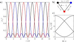
Figure 6: a) Optical amplitudes $|A_{j}|^{2}$. The initial state has one photon on site $1$. For $\Phi=-\pi/2$, the initial excitation moves counterclockwise around the triangular plaquette shown in b). For $\Phi=\pi/2$, the initial excitation would move clockwise around the triangle. c) Dispersion relation $\Omega_{k}$ as a function of the phase $\Phi$.

The Hamiltonian of the three-site model can be diagonalized best after going into a rotating frame by applying the transformation

$$U=e^{it\sum_{j}\nu_{j}^{\phantom{{\dagger}}}a_{j}^{{\dagger}}a_{j}^{\phantom{{\dagger}}}}e^{it\sum_{l}\omega_{l}^{\phantom{{\dagger}}}b_{l}^{{\dagger}}b_{l}^{\phantom{{\dagger}}}}\,,$$ (26)

to Eq. (16) which leads to the Hamiltonian

$$H =J_{12}B_{12}\left(e^{-i\phi_{12}}a_{1}^{{\dagger}}a_{2}^{\phantom{{\dagger}}}+{\rm{H.c.}}\right)+J_{23}B_{23}\left(e^{-i\phi_{23}}a_{2}^{{\dagger}}a_{3}^{\phantom{{\dagger}}}+{\rm{H.c.}}\right)+J_{13}B_{13}\left(e^{i\phi_{13}}a_{3}^{{\dagger}}a_{1}^{\phantom{{\dagger}}}+{\rm{H.c.}}\right)\,.$$ (27)

Since we are here interested in the eigenvalues, we can perform a gauge transform $a_{j}\to a_{j}e^{i\chi_{j}}$ and make the following gauge choice

$$-\phi_{12}+\chi_{2}-\chi_{1} =\tilde{\Phi}\,,$$ (28)

$$-\phi_{23}+\chi_{3}-\chi_{2} =\tilde{\Phi}\,,$$ (29)

$$\phi_{13}+\chi_{1}-\chi_{3} =\tilde{\Phi}\,,$$ (30)

which we can write as $\phi_{13}-\phi_{12}-\phi_{23}=3\tilde{\Phi}=\Phi$. The Hamiltonian can then be written as

$$H=\sum_{j=1}^{3}J_{j}B_{j}e^{i\tilde{\Phi}}a_{j}^{{\dagger}}a_{j+1}^{\phantom{{\dagger}}}+{\rm{H.c.}}\,,$$ (31)

where we assumed periodic boundary conditions, i.e., $a_{4}=a_{1}$ and for convenience we introduce $J_{12,23,13}\to J_{1,2,3}$ and similarly for $B_{12,23,13}$. By introducing normal modes

$$a_{j}^{{\dagger}}=\frac{1}{\sqrt{3}}\sum_{k=0}^{2}e^{-2\pi ikj/3}A_{k}^{{\dagger}}\,,$$ (32)

$$A_{k}^{{\dagger}}=\frac{1}{\sqrt{3}}\sum_{j=1}^{3}e^{2\pi ikj/3}a_{j}^{{\dagger}}\,,$$ (33)

and furthermore assuming equal tunneling amplitude $J$ and limit-cycle amplitude $B$, the Hamiltonian can be diagonalized

$$H=\sum_{k=0}^{2}\Omega_{k}^{\phantom{{\dagger}}}A_{k}^{{\dagger}}A_{k}^{\phantom{{\dagger}}}\,,$$ (34)

where $\Omega_{k}=2JB\cos\left(\Phi/3+2\pi k/3\right)$. As already pointed out in Ref. Koch2010, , for $\Phi=\pm\pi/2$ this setup shows the behaviour of a photon circulator.

Appendix C Spectrum of a Periodic Trajectory Versus a Chaotic Trajectory

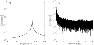
Figure 7: Fourier transform of the trajectories shown in Fig. 3 a) and Fig. 3 b). In a) the spectrum shows a clear peak indicating a periodic trajectory, cf. Fig. 3 a). In b) however the spectrum is flat which indicates a chaotic trajectory, cf. Fig. 3 b).

Here, we give additional information on how we made the distinction between the periodic and chaotic behavior of the dynamical gauge field in the case of the three-site model. In the main text, we chose to present the distinction, periodic versus chaotic, by plotting the bifurcation diagram shown in Fig. 3 c). In addition to this, we also investigated the Fourier transform of the time series $\Phi(t)$, the spectrum. For a periodic time series there is a pronounced peak in the spectrum at the frequency corresponding to the period of the time series. In the case of a chaotic time series the spectrum does not show a preferred frequency and is almost flat. In Fig. 7 a) and Fig. 7 b), we show the Fourier transform of the time series corresponding to the phase space trajectories shown in Fig. 3 a) and Fig. 3 b), respectively. In the case of a periodic trajectory, the spectrum clearly shows a peak, where as for a chaotic trajectory the spectrum is flat. To summarize, in addition to the bifurcation diagram presented in the main text, we also checked the Fourier transform of the time series to consistently distinguish periodic from chaotic trajectories.

Appendix D The Triangular Lattice: Equations of Motion

On a two-dimensional triangular lattice we denote dynamical variables on lattice site $n,m$ with a subscripts $(n,m)$ and dynamical variables on the directed links from site $n,m$ to site $k,l$ by a subscript $(n,m)(k,l)$. The equations of motion for the mechanical phases $\phi_{(n,m)(n,m+1)}$ on the lattice links are

$$\dot{\phi}_{(n,m)(n,m+1)}=-\omega_{(n,m)(n,m+1)}-\frac{J_{(n,m)(n,m+1)}}{B_{(n,m)(n,m+1)}}A_{n,m}A_{n,m+1}\cos(\phi_{(n,m)(n,m+1)}+\theta_{n,m}-\theta_{n,m+1})\,,$$

$$\dot{\phi}_{(n,m+1)(n+1,m)}=-\omega_{(n,m+1)(n+1,m)}-\frac{J_{(n,m+1)(n+1,m)}}{B_{(n,m+1)(n+1,m)}}A_{n,m+1}A_{n+1,m}\cos(\phi_{(n,m+1)(n+1,m)}+\theta_{n,m+1}-\theta_{n+1,m})\,,$$

$$\dot{\phi}_{(n,m)(n+1,m)}=-\omega_{(n,m)(n+1,m)}-\frac{J_{(n,m)(n+1,m)}}{B_{(n,m)(n+1,m)}}A_{n,m}A_{n+1,m}\cos(\phi_{(n,m)(n+1,m)}+\theta_{n,m}-\theta_{n+1,m})\,.$$

The optical amplitudes $A_{n,m}$ obey the equations of motion

$$\dot{A}_{n,m}= -J_{(n,m)(n,m+1)}B_{(n,m)(n,m+1)}\sin(\phi_{(n,m)(n,m+1)}+\theta_{n,m}-\theta_{n,m+1})A_{n,m+1}$$ (35)

$$-J_{(n,m)(n+1,m)}B_{(n,m)(n+1,m)}\sin(\phi_{(n,m)(n+1,m)}+\theta_{n,m}-\theta_{n+1,m})A_{n+1,m}$$

$$+J_{(n,m-1)(n,m)}B_{(n,m-1)(n,m)}\sin(\phi_{(n,m-1)(n,m)}+\theta_{n,m-1}-\theta_{n,m})A_{n,m-1}$$

$$-J_{(n,m)(n+1,m-1)}B_{(n,m)(n+1,m-1)}\sin(\phi_{(n,m)(n+1,m-1)}+\theta_{n,m}-\theta_{n+1,m-1})A_{n+1,m-1}$$

$$+J_{(n-1,m)(n,m)}B_{(n-1,m)(n,m)}\sin(\phi_{(n-1,m)(n,m)}+\theta_{n-1,m}-\theta_{n,m})A_{n-1,m}$$

$$+J_{(n-1,m+1)(n,m)}B_{(n-1,m+1)(n,m)}\sin(\phi_{(n-1,m+1)(n,m)}+\theta_{n-1,m+1}-\theta_{n,m})A_{n-1,m+1}\,,$$

and the optical phases $\theta_{n,m}$ on a lattice site evolve according to

$$\dot{\theta}_{n,m}= -\nu_{n,m}$$ (36)

$$-J_{(n,m)(n,m+1)}B_{(n,m)(n,m+1)}\frac{A_{n,m+1}}{A_{n,m}}\cos(\phi_{(n,m)(n,m+1)}+\theta_{n,m}-\theta_{n,m+1})$$

$$-J_{(n,m)(n+1,m)}B_{(n,m)(n+1,m)}\frac{A_{n+1,m}}{A_{n,m}}\cos(\phi_{(n,m)(n+1,m)}+\theta_{n,m}-\theta_{n+1,m})$$

$$-J_{(n,m-1)(n,m)}B_{(n,m-1)(n,m)}\frac{A_{n,m-1}}{A_{n,m}}\cos(\phi_{(n,m-1)(n,m)}+\theta_{n,m-1}-\theta_{n,m})$$

$$-J_{(n,m)(n+1,m-1)}B_{(n,m)(n+1,m-1)}\frac{A_{n+1,m-1}}{A_{n,m}}\cos(\phi_{(n,m)(n+1,m-1)}+\theta_{n,m}-\theta_{n+1,m-1})$$

$$-J_{(n,m)(n+1,m-1)}B_{(n,m)(n+1,m-1)}\frac{A_{n-1,m}}{A_{n,m}}\cos(\phi_{(n,m)(n+1,m-1)}+\theta_{n-1,m}-\theta_{n,m})$$

$$-J_{(n-1,m+1)(n,m)}B_{(n-1,m+1)(n,m)}\frac{A_{n-1,m+1}}{A_{n,m}}\cos(\phi_{(n-1,m+1)(n,m)}+\theta_{n-1,m+1}-\theta_{n,m})\,.$$

A driving term on a particular site and dissipation of the photons on each site can be added straightforwardly, as also done for the three-site model.

Appendix E The Triangular Lattice: Distribution of Optical and Mechanical Frequencies

As mentioned in the main text, the links are directed: A photon tunneling from a site with a low (high) on-site frequency to a site with a high (low) on-site frequency absorbs (emits) a phonon. These processes have to be resonant which could be achieved by distributing the photon and phonon frequencies in the right way. For instance, the frequencies can be arranged as shown in Fig. 8.

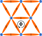
Figure 8: Possible distribution of optical (blue dots) and mechanical (orange ellipses) frequencies on a $3\times 3$ triangular lattice as an example.

References

- (1) Aspelmeyer M, Kippenberg T J and Marquardt F 2014 Rev. Mod. Phys. 86 1391
- (2) Teufel J D, Donner T, Li D, Harlow J W, Allman M S, Cicak K, Sirois A J, Whittaker J D, Lehnert K W and Simmonds R W 2011 Nature 475 359
- (3) Chan J, Mayer Alegre T P, Safavi-Naeini A H, Hill J T, Krause A, Gröblacher S, Aspelmeyer M and Painter O 2011 Nature 478 89
- (4) Teufel J D, Donner T, Castellanos-Beltran M A, Harlow J W and Lehnert K W 2009 Nat. Nanotechnol. 4 820
- (5) Manipatruni S, Robinson J T and Lipson M 2009 Phys. Rev. Lett. 102 213903
- (6) Habraken S J M, Stannigel K, Lukin M D, Zoller P and Rabl P 2012 New J. Phys. 14 115004
- (7) Hafezi M and Rabl P 2012 Opt. Express 20 7672
- (8) Wang Z, Shi L, Liu Y, Xu X and Zhang X 2015 Scientific Reports 5 8657
- (9) Ruesink F, Miri M-A, Alù A and Verhagen E 2016 arXiv:1607.07180
- (10) Fang K, Luo J, Metelmann A, Matheny M H, Marquardt F, Clerk A A and Painter O 2016 arXiv:1608.03620
- (11) Bhattacharya S and P. Meystre P 2008 Phys. Rev. A 78 041801
- (12) Chang D E, Safavi-Naeini A H, Hafezi M and Painter O 2011 New J. Phys. 13 023003
- (13) Xuereb A, Genes C and Dantan A 2012 Phys. Rev. Lett. 109 223601
- (14) Tomadin A, Diehl S, Lukin M D, Rabl P and Zoller P 2012 Phys. Rev. A 86 033821
- (15) Schmidt M, Ludwig M and Marquardt F 2012 New J. Phys. 14 125005
- (16) Akram U, Munro W, Nemoto K and Milburn G J 2012 Phys. Rev. A 86 042306
- (17) Chen W and Clerk A A 2014 Phys. Rev. A 89 033854
- (18) Schmidt M, Peano V and Marquardt F 2015 New J. Phys. 17 023025
- (19) Schmidt M, Keßler S, Peano V, Painter O and Marquardt F 2015 Optica 2 635
- (20) Peano V, Brendel C, Schmidt M and Marquardt F 2015 Phys. Rev. X 5 031011
- (21) Raghu S and Haldane F D M 2008 Phys. Rev. Lett. 100 013904
- (22) Wang Z, Chong Y, Joannopoulos J D and Soljačić M 2009 Nature 461 772
- (23) Koch J, Houck A A, Le Hur K and Girvin S M 2010 Phys. Rev. A 82 043811
- (24) Umucallar R O and Carusotto I 2011 Phys. Rev. A 84 043804
- (25) Hafezi M, Demler E A, Lukin M D and Taylor J M 2011 Nat. Phys. 7 907
- (26) Fang K, Yu Z and Fan S 2012 Nature Photon. 6 782
- (27) Hafezi M, Mittal S, Fan J, Migdall A and Taylor J M 2013 Nature Photon. 7 1001
- (28) Rechtsman M C, Zeuner J M, Tünnermann A, Nolte S, Segev M and Szameit A 2013 Nature Photon. 7 153
- (29) Lu L, Joannopoulos J D and Soljačić M 2014 Nature Photon. 8 821
- (30) Mittal S, Fan J, Faez S, Migdall A, Taylor J M and Hafezi M 2014 Phys. Rev. Lett. 113 087403
- (31) Jaksch D and Zoller P 2003 New J. Phys. 5 56
- (32) Sørensen A A, Demler E A and Lukin M D 2005 Phys. Rev. Lett. 94 086803
- (33) Lin Y-J, Compton R L, Jiménez-García K, Porto J V and Spielman I B 2009 Nature 462 628
- (34) Aidelsburger M, Atala M, Nascimbène S, Trotzky S, Chen Y-A and Bloch I 2011 Phys. Rev. Lett. 107 255301
- (35) Aidelsburger M, Atala M, Lohse M, Barreiro J T, Paredes B and Bloch I 2013 Phys. Rev. Lett. 111 185301
- (36) Jotzu G, Messer M, Desbuquois R, Lebrat M, Uehlinger T, Greif D and Esslinger T 2014 Nature 515 237
- (37) Osterloh K, Baig M, Santos L, Zoller P and Lewenstein M 2005 Phys. Rev. Lett. 95 010403
- (38) Ruseckas J, Juzelinas G, Öhberg P and Fleischhauer M 2005 Phys. Rev. Lett. 95 010404
- (39) Zohar E and Reznik B 2011 Phys. Rev. Lett. 107 275301
- (40) Hauke P, Tieleman O, Celi A, Ölschläger C, Simonet J, Struck J, Weinberg M, Windpassinger P, Sengstock K, Lewenstein M and Eckardt A 2012 Phys. Rev. Lett. 109 145301
- (41) Banerjee D, Dalmonte M, Müller M, Rico E, Stebler P, Wiese U J and Zoller P 2012 Phys. Rev. Lett. 109 175302
- (42) Zohar E, Cirac J I and Reznik B 2013 Phys. Rev. Lett. 110 055302
- (43) Edmonds M J, Valiente M, Juzelinas G, Santos L and Öhberg P 2013 Phys. Rev. Lett. 110 085301
- (44) Marcos D, Rabl P, Rico E and Zoller P 2013 Phys. Rev. Lett. 111 110504
- (45) Marcos D, Widmer P, Rico E, Hafezi M, Rabl P, Wiese U J and Zoller P 2014 Annals of Physics 351 634
- (46) Wiese U J 2013 Ann. der Phys. 525 777
- (47) Zohar E, Cirac J I and Reznik B 2015 Rep. Prog. Phys. 79 014401
- (48) Lauter R, Brendel C, Habraken S J M, and Marquardt F 2015 Phys. Rev. E 92 012902
- (49) Eichenfield M, Chan J, Camacho R M, Vahala K J and Painter O 2009 Nature 462 78
- (50) Safavi-Naeini A H and Painter O 2010 Opt. Express 18 14926
- (51) Safavi-Naeini A H, Mayer Alegre T P, Winger M and Painter O 2010 Appl. Phys. Lett. 97 181106
- (52) Gavartin E, Braive R, Sagnes I, Arcizet O, Beveratos A, Kippenberg T J and Robert-Philip I 2011 Phys. Rev. Lett. 106 203902
- (53) Safavi-Naeini A H, Hill J T, Meenehan S, Chan J, Gröblacher S and Painter O 2014 Phys. Rev. Lett. 112 153603
- (54) Zhang M, Shah S, Cardenas J and Lipson M 2015 Phys. Rev. Lett. 115 163902
- (55) Safavi-Naeini A H and Painter O 2011 New J. Phys. 13 013017
- (56) Marquardt F, Harris J G E and Girvin S M 2006 Phys. Rev. Lett. 96 103901
- (57) Roque T F, Peano V, Yevtushenko O M and Marquardt F 2016 arXiv:1607.04159
- (58) Heinrich G, Ludwig M, Qian J, Kubala B and Marquardt F 2011 Phys. Rev. Lett. 107 043603
- (59) Ludwig M and Marquardt F 2013 Phys. Rev. Lett. 111 073603