Intrinsic alignments of BOSS LOWZ galaxies II: Impact of shape measurement methods

Abstract

Measurements of intrinsic alignments of galaxy shapes with the large-scale density field, and the inferred intrinsic alignments model parameters, are sensitive to the shape measurement methods used. In this paper we measure the intrinsic alignments of the Sloan Digital Sky Survey-III (SDSS-III) Baryon Oscillation Spectroscopic Survey (BOSS) LOWZ galaxies using three different shape measurement methods (re-Gaussianization, isophotal, and de Vaucouleurs), identifying a variation in the inferred intrinsic alignments amplitude at the 40% level between these methods, independent of the galaxy luminosity or other properties. We also carry out a suite of systematics tests on the shapes and their two-point correlation functions, identifying a pronounced contribution from additive PSF systematics in the de Vaucouleurs shapes. Since different methods measure galaxy shapes at different effective radii, the trends we identify in the intrinsic alignments amplitude are consistent with the interpretation that the outer regions of galaxy shapes are more responsive to tidal fields, resulting in isophote twisting and stronger alignments for isophotal shapes. We observe environment dependence of ellipticity, with brightest galaxies in groups being rounder on average compared to satellite and field galaxies. We also study the anisotropy in intrinsic alignments measurements introduced by projected shapes, finding effects consistent with predictions of the nonlinear alignment model and hydrodynamic simulations. The large variations seen using the different shape measurement methods have important implications for intrinsic alignments forecasting and mitigation with future surveys.

1 Introduction

Weak gravitational lensing (for a review, see Massey et al., 2010; Weinberg et al., 2013), the deflection of light from distant objects by mass in more nearby foregrounds, results in coherent distortions of galaxy shapes that are measured statistically, by averaging over large ensembles of galaxies. It has the power to reveal the dark matter halos in which galaxies and galaxy clusters reside (e.g., Velander et al., 2014; Coupon et al., 2015; Han et al., 2015; Hudson et al., 2015; Zu & Mandelbaum, 2015), to constrain the growth of cosmic structure and thus the nature of dark energy (e.g., Heymans et al., 2013; Jee et al., 2013; Mandelbaum et al., 2013), and even to constrain the theory of gravity on cosmological scales (e.g., Reyes et al., 2010; Simpson et al., 2013; Pullen et al., 2015). Intrinsic alignments of galaxies (IA; for a review, see Joachimi et al. 2015; Troxel & Ishak 2015; Kirk et al. 2015; Kiessling et al. 2015), the coherent alignment of galaxy shapes with each other (II) or with the local density field (GI), result in a violation of the assumption that galaxy shapes are not intrinsically correlated and that any observed shape correlations are from gravitational lensing. Thus, intrinsic alignments are an important astrophysical systematic for weak lensing surveys.

Singh et al. (2015) (hereafter Paper I) studied the IA of galaxies in one of the Sloan Digital Sky Survey-III (SDSS-III) Baryon Oscillation Spectroscopic Survey (BOSS) galaxy samples, called LOWZ. This sample consists of Luminous Red Galaxies (LRGs) with a comoving number density of $\sim 3\times 10^{-4}(h/\text{Mpc})^{3}$ from $0.16<z<0.36$. The large sample size and high signal-to-noise ratio enabled not only a detection of IA, but a study of its dependence on galaxy properties such as mass, luminosity and environment, finding strong correlations of IA with the host halo mass and galaxy luminosity (see also Joachimi et al., 2011). A commonly-adopted theoretical model called the linear alignment model (Catelan et al., 2001; Hirata & Seljak, 2003), which relates the galaxy alignments to the tidal field from large-scale structure at the time of galaxy formation, was found to provide a good description of the data for projected separation $r_{p}>6~{}h^{-1}$Mpc, provided that the non-linear matter power spectrum was used (NLA model; Bridle & King, 2007).

A natural goal of such studies is to predict the intrinsic alignment contamination in weak lensing surveys, and to provide templates that can be used to marginalize over this effect. However, different IA studies in the literature (e.g., Mandelbaum et al., 2006; Hirata et al., 2007; Okumura et al., 2009; Joachimi et al., 2011; Blazek et al., 2011; Hao et al., 2011; Hung & Ebeling, 2012; Li et al., 2013; Chisari et al., 2014; Sifón et al., 2015; Singh et al., 2015) use different galaxy shape measurement methods and ensemble IA estimators, which makes it difficult to compare them or to combine their results into a single comprehensive view of the subject. For example, Okumura et al. (2009) used isophotal shape measurements from SDSS data release 7 (DR7) to measure shape-shape correlations for the SDSS LRG sample at high significance which were then interpreted by Blazek et al. (2011) in the context of the NLA model. However, in Paper I  using re-Gaussianization shapes and a larger BOSS low redshift sample (LOWZ-DR11) from SDSS-III, we measured the shape-shape correlation function to be consistent with zero. Though the two measurements were shown to be statistically consistent in Paper I, the reason for the varying detection significance in the two studies is not well understood, and worth investigation.

IA measurements with different shape measurements may be particularly difficult to compare due to different systematic errors and ranges of galaxy radius probed by different methods. First, galaxy shape measurements are affected by observational systematics such as the point-spread function (PSF), pixel noise, errors in estimation and subtraction of sky level, and blending with the light profiles of nearby galaxies. Different shape measurement methods treat these systematics differently or in some cases ignore them. Improper treatment of systematic effects in galaxy shapes can propagate into IA measurements. For example, Hao et al. (2011) found that using isophotal shapes from the SDSS to measure the alignments of satellite shapes around brightest cluster galaxies (BCGs) that these alignments correlated with the apparent magnitude of the BCG. This result was interpreted as a systematic error in isophotal shapes of satellite galaxies from BCG light leaking into the satellite shapes, an effect that is more complicated than a multiplicative bias.

Also, different shape measurement methods use different radial weight functions and thus probe galaxy shapes at different effective radii. Intrinsic variation in the galaxy shapes with radius can thus affect the IA measurements. These could be gradients in the ellipticity with radius (with galaxies being intrinsically more or less round in the outer regions), or isophotal twisting due to the outer parts of galaxies being more aligned with external tidal field than the inner parts. For example, Tenneti et al. (2015) found in hydrodynamic simulations that galaxies become rounder in their outer regions. Velliscig et al. (2015b), on the other hand, found that the projected RMS ellipticity, $e_{\text{rms}}$, is lower when measured using star particles within the half-light radius compared to using all star particles (see also Chisari et al., 2015). In observations, the magnitude and sign of ellipticity gradients have been found to be correlated with the galaxy environment (di Tullio, 1978, 1979; Pasquali et al., 2006). Ellipticity variations using different shape measurements will affect inferences made using ensemble IA estimators that include the ellipticity rather than just the position angle (e.g., Mandelbaum et al., 2006; Hirata et al., 2007; Joachimi et al., 2011; Blazek et al., 2011; Singh et al., 2015).

Several studies have also detected isophote twists in small samples of elliptical galaxies, whereby the position angle in the measured galaxy shape changes with radius (Wyatt, 1953; Abramenko, 1978; Kormendy, 1982; Fasano & Bonoli, 1989; Nieto et al., 1992; Lauer et al., 2005). The isophote twisting may originate from varying triaxiality of galaxies with radii (see, e.g., Romanowsky & Kochanek, 1998) though Kormendy (1982) pointed out that the outer regions of galaxies are more susceptible to tidal fields, which can result in isophote twisting. In simulations, Kuhlen et al. (2007) observed the effects of shape twisting from tidal interaction when measuring the radial alignments of dark matter subhalos. The radial alignment signal of subhaloes increased monotonically with the radius at which the subhalo shape was measured. If such results also apply to galaxies, then a stronger IA signal from shape measurements that probe the outer regions of galaxies would be expected. In support of this inference, Velliscig et al. (2015a) found using hydrodynamic simulations that using star particles within the half-light radius to define the galaxy shapes results in lower IA signal compared to using all the star particles (see also Chisari et al., 2015, but note that that work attributes the differences to ellipticity variations rather than to isophote twists).

Finally, we measure only the projected shapes of galaxies, which are insensitive to line-of-sight galaxy alignments. This effect introduces anisotropy in the redshift-space structure of IA, and different estimators of IA vary in their sensitivity to this anisotropy. For example, the redshift-space structure of the 3D shape-density cross-correlation function, $\xi_{g+}$, includes the redshift-space structure of the 3D galaxy-galaxy auto-correlation function, $\xi_{gg}$; however, the mean IA shear, $\langle\gamma\rangle$, is independent of $\xi_{gg}$ ($\xi_{g+}=\langle\gamma\rangle(1+\xi_{gg})$, Blazek et al. 2015). Depending on the relative importance of variations in IA and galaxy clustering, $\xi_{g+}$ and $\langle\gamma\rangle$ may have different redshift-space structure. The variations in the sensitivity to redshift-space structure between different IA estimators can complicate a quantitive comparisons between studies using different estimators.

In this paper, we repeat the analysis of Paper I using three different shape measurement methods, and carry out numerous systematics tests, to study the radial and environment dependence of galaxy shapes and of the IA signal. We also use the methodology of Blazek et al. (2011) to understand the origin of differences in their shape-shape correlations ($w_{++}$) measurement and the one in Paper I. Finally, to understand the redshift-space structure of intrinsic alignments, we investigate the IA signals as a function of projected and line of sight separations and compare the results with NLA model predictions.

Throughout we use a standard flat $\Lambda$CDM cosmology with $h=0.7$, $\Omega_{b}=0.046$, $\Omega_{DM}=0.236$, $\Omega_{\Lambda}=0.718$, $n_{s}=0.9646$, $\sigma_{8}=0.817$ (WMAP9, Hinshaw et al., 2013). All distances are in comoving $h^{-1}\text{Mpc}$, though $h=0.7$ was used to calculate absolute magnitudes and to generate predictions for the matter power spectrum.

2 Formalism and Methodology

Details of intrinsic alignments models and correlation estimators are given in Paper I. In this section, we briefly summarize the important points.

2.1 The nonlinear alignment (NLA) model

The linear alignment (LA) model predicts that IA are set at the time of galaxy formation (Catelan et al., 2001), with galaxy shapes being aligned with the tidal fields present during galaxy formation. This assumption allows us to write intrinsic shear in terms of primordial potential $\phi_{p}$

$$\gamma^{I}=(\gamma^{I}_{+},\gamma^{I}_{\times})=-\frac{C_{1}}{4\pi G}(\partial^{2}_{x}-\partial^{2}_{y},\partial_{x}\partial_{y})\phi_{p},$$ (1)

with alignment strength defined by an amplitude parameter $C_{1}$. In our sign convention, positive (negative) $\gamma^{I}_{+}$ indicates alignments along (perpendicular to) the direction of the tidal field while positive (negative) $\gamma^{I}_{\times}$ indicates alignments along the direction at $45$ ($135$) degrees from the direction of the tidal field. Assuming a linear galaxy bias relating matter overdensities $\delta_{m}$ and galaxy densities $\delta_{g}=b~{}\delta_{m}$, the power spectrum of galaxy-shape and shape-shape correlations can be written as (Hirata & Seljak, 2003)

$$P_{g+}(\vec{k},z) =A_{I}b\frac{C_{1}\rho_{\text{crit}}\Omega_{m}}{D(z)}\frac{k_{x}^{2}-k_{y}^{2}}{k^{2}}P_{\delta}^{\text{lin}}(\vec{k},z)$$ (2)

$$P_{++}(\vec{k},z) =f_{II}\left(A_{I}\frac{C_{1}\rho_{\text{crit}}\Omega_{m}}{D(z)}\frac{k_{x}^{2}-k_{y}^{2}}{k^{2}}\right)^{2}P_{\delta}^{\text{lin}}(\vec{k},z)$$ (3)

$$P_{g\times}(\vec{k},z) =A_{I}b\frac{C_{1}\rho_{\text{crit}}\Omega_{m}}{D(z)}\frac{k_{x}k_{y}}{k^{2}}P_{\delta}^{\text{lin}}(\vec{k},z)$$ (4)

$P_{\delta}^{\text{lin}}$ is the linear matter power spectrum. $P_{g+}$ ($P_{g\times}$) is the cross-power spectrum between the galaxy density field and the shear component along (at $45^{\circ}$ from) the line joining the galaxy pair. $P_{++}$ is the shape-shape correlation with shear component along the line joining the galaxy pair. Following Joachimi et al. (2011), we fix $C_{1}\rho_{\text{crit}}=0.0134$ and use a dimensionless constant $A_{I}$ to measure the IA amplitude, which is primarily constrained from density-shape cross-correlations. To allow for departure from the LA model, we have introduced an additional free parameter $f_{II}$, which would be 1 in the case that the LA model is correct. In the NLA model, to extend the linear alignment model to the non-linear regime, the linear matter power spectrum is replaced with the non-linear matter power spectrum (Bridle & King, 2007) using an updated halo-fit model (Smith et al., 2003; Takahashi et al., 2012). As shown by Blazek et al. (2015), the NLA model neglects other terms that are important at the same order; however, in Paper I we found it provided an adequate fit to our intrinsic alignments measurements down to $\sim 6$ $h^{-1}\mathrm{Mpc}$.

The power spectra in Eqs. (2)–(4) can be Fourier transformed to obtain the 3D correlation functions as a function of comoving projected separation $r_{p}$ and line-of-sight separation $\Pi$,

$$\xi_{AB}(r_{p},\Pi,z)= \int\frac{\mathrm{d}^{2}k_{\perp}\mathrm{d}k_{z}}{(2\pi)^{3}}P_{AB}(\vec{k},z)\left(1+\beta_{A}\mu^{2}\right)$$

$$\left(1+\beta_{B}\mu^{2}\right)e^{i(r_{p}.k_{\perp}+\Pi k_{z})}.$$ (5)

The Kaiser factor ($1+\beta\mu^{2}$) accounts for the effect of linear redshift-space distortions (RSD; Kaiser 1987). As shown in Paper I, for power spectra that include intrinsic shapes, $\beta_{+,\times}=0$ (the shear field is not affected by RSD to first order). For galaxies, $\beta(z)=f(z)/b$, where the linear growth factor $f(z)\sim\Omega_{m}(z)^{0.55}$ in the $\Lambda$CDM model.

In the data, we measure the projected correlation function, $w_{AB}(r_{p})$, which can be obtained by projecting the 3D correlation function in Eq. (5) along the line-of-sight separation:

$$w_{AB}(r_{p})= \int\mathrm{d}z\,W(z)\int\mathrm{d}\Pi\,\xi_{AB}(r_{p},\Pi,z).$$ (6)

$W(z)$ is the redshift window function (Mandelbaum et al., 2011)

$$W(z)=\frac{p_{A}(z)p_{B}(z)}{\chi^{2}(z)\mathrm{d}\chi/\mathrm{d}z}\left[\int\frac{p_{A}(z)p_{B}(z)}{\chi^{2}(z)\mathrm{d}\chi/\mathrm{d}z}\mathrm{d}z\right]^{-1}$$ (7)

Assuming cross-correlation between samples of galaxies with shapes S and others that trace the density field D with in principle different biases $b_{S}$ and $b_{D}$, the different projected correlation functions are

$$w_{gg}(r_{p})=\frac{b_{S}b_{D}}{\pi^{2}}\int\mathrm{d}z\,{W(z)}\int_{0}^{\infty}\mathrm{d}k_{z}\int_{0}^{\infty}\mathrm{d}k_{\perp}\frac{k_{\perp}}{k_{z}}P(\vec{k},z)$$

$$\sin(k_{z}\Pi_{\text{max}})J_{0}(k_{\perp}r_{p})\left(1+\beta_{S}\mu^{2}\right)\left(1+\beta_{D}\mu^{2}\right)$$ (8)

$$w_{g+}(r_{p})=\frac{A_{I}b_{D}C_{1}\rho_{\text{crit}}\Omega_{m}}{\pi^{2}}\int\mathrm{d}z\frac{W(z)}{D(z)}\int_{0}^{\infty}\mathrm{d}k_{z}\int_{0}^{\infty}\mathrm{d}k_{\perp}$$

$$\frac{k_{\perp}^{3}}{(k_{\perp}^{2}+k_{z}^{2})k_{z}}P(\vec{k},z)\sin(k_{z}\Pi_{\text{max}})J_{2}(k_{\perp}r_{p})\left(1+\beta_{D}\mu^{2}\right)$$ (9)

$$w_{++}(r_{p})=f_{II}\frac{\left(A_{I}C_{1}\rho_{\text{crit}}\Omega_{m}\right)^{2}}{2\pi^{2}}\int\mathrm{d}z\frac{W(z)}{D(z)^{2}}\int_{0}^{\infty}\mathrm{d}k_{z}\int_{0}^{\infty}\mathrm{d}k_{\perp}$$

$$\frac{k_{\perp}^{5}}{(k_{\perp}^{2}+k_{z}^{2})^{2}k_{z}}P(\vec{k},z)\sin(k_{z}\Pi_{\text{max}})\times[J_{0}(k_{\perp}r_{p})+J_{4}(k_{\perp}r_{p})]$$ (10)

Whether we fit the three correlation functions ($w_{gg}$, $w_{g+}$, and $w_{++}$) jointly or independently to this model, the galaxy bias, intrinsic alignment amplitude $A_{I}$, and $f_{II}$ are primarily constrained by $w_{gg}$, $w_{g+}$, and $w_{++}$, respectively. This is due to the different sensitivities of these signals to the three parameters, along with the different signal-to-noise ratio ($S/N$) in the measurements. The $S/N$ degrades with increasing factors of galaxy shape due to the shape noise they add to the correlation function.

2.2 Correlation function estimators

We calculate cross-correlation functions between sets of galaxies for which we wish to estimate the intrinsic alignments (the “shape sample”) and those used to trace the density field (the “density sample”). We use a generalized Landy-Szalay estimator (Landy & Szalay, 1993) to compute the correlation functions:

$$\xi_{gg}=\frac{(S-R_{S})(D-R_{D})}{R_{S}R_{D}} =\frac{SD-R_{S}D-SR_{D}}{R_{S}R_{D}}+1$$

$$\xi_{g+} =\frac{S_{+}D-S_{+}R_{D}}{R_{S}R_{D}}$$

$$\xi_{++} =\frac{S_{+}S_{+}}{R_{S}R_{S}},$$

where $S$ and $D$ represent the galaxy counts in the shape and density samples, and $R_{S}$ and $R_{D}$ are sets of random points corresponding to these samples. The terms involving shears for the galaxies are

$$S_{+}X =\sum_{i\in S,j\in X}\gamma_{+}^{(i)}(j|i),$$

$$S_{+}S_{+} =\sum_{i\in S,j\in S}\gamma_{+}^{(i)}(i|j)\gamma_{+}^{(j)}(j|i).$$

Here $\gamma_{+}^{(i)}(j|i)$ represents the component of the shear for galaxy $i$ along the line joining it to galaxy $j$. Positive (negative) $\gamma_{+}$ implies radial (tangential) alignments.

Measuring projected correlations involves summation over bins in $\Pi$,

$$w_{AB}=\int^{\Pi_{\text{max}}}_{-\Pi_{\text{max}}}\xi_{AB}(r_{p},\Pi)\,\mathrm{d}\Pi.$$ (11)

We use $\Pi_{\text{max}}=100h^{-1}\text{Mpc}$ and $d\Pi=10h^{-1}\text{Mpc}$.

To calculate the covariance matrices of the $w_{AB}$, we divide the sample into 100 equal-area regions, compute the signal by excluding one region at a time and then compute the jackknife variance from the 100 jackknife samples. See Paper I for more details.

2.3 Anisotropy

It is well known that redshift-space distortions (RSD) introduce anisotropy in the observed galaxy clustering in redshift space (e.g., Kaiser, 1987; Beutler et al., 2014). In Paper I, it was shown that the IA measurements are not affect by RSD to first order. However, IA are affected by another source of anisotropy, the projected shapes of galaxies, due to which we cannot measure the line-of-sight IA signal. Hence, the IA signal is expected to fall faster with increasing line-of-sight separation, $\Pi$, than with $r_{p}$.

To understand this anisotropy, we study the IA signal in $(r_{p},\Pi)$ space and compare it with the NLA model prediction. To compute the model predictions, we compute the real part of $\xi_{AB}$ as follows:

$$\xi_{gg}(r_{p},\Pi)= \frac{b_{S}b_{D}}{2\pi^{2}}\int\mathrm{d}z\,{W(z)}\int_{0}^{\infty}\mathrm{d}k_{z}\cos(k_{z}\Pi)$$

$$\int_{0}^{\infty}\mathrm{d}k_{\perp}\frac{k_{\perp}}{k_{z}}P(\vec{k},z)J_{0}(k_{\perp}r_{p})\left(1+\beta_{S}\mu^{2}\right)$$

$$\left(1+\beta_{D}\mu^{2}\right)$$ (12)

$$\xi_{g+}(r_{p},\Pi)= \frac{A_{I}b_{D}C_{1}\rho_{\text{crit}}\Omega_{m}}{2\pi^{2}}\int\mathrm{d}z\frac{W(z)}{D(z)}\int_{0}^{\infty}\mathrm{d}k_{z}\cos(k_{z}\Pi)$$

$$\int_{0}^{\infty}\mathrm{d}k_{\perp}\frac{k_{\perp}^{3}}{(k_{\perp}^{2}+k_{z}^{2})k_{z}}P(\vec{k},z)J_{2}(k_{\perp}r_{p})$$

$$\left(1+\beta_{D}\mu^{2}\right)$$ (13)

$$\xi_{++}(r_{p},\Pi)= f_{II}\frac{\left(A_{I}C_{1}\rho_{\text{crit}}\Omega_{m}\right)^{2}}{4\pi^{2}}\int\mathrm{d}z\frac{W(z)}{D(z)^{2}}\int_{0}^{\infty}\mathrm{d}k_{z}$$

$$\cos(k_{z}\Pi)\int_{0}^{\infty}\mathrm{d}k_{\perp}\frac{k_{\perp}^{5}}{(k_{\perp}^{2}+k_{z}^{2})^{2}k_{z}}P(\vec{k},z)\times$$

$$[J_{0}(k_{\perp}r_{p})+J_{4}(k_{\perp}r_{p})]$$ (14)

The $k_{\perp}^{2}/k^{2}$ terms in Eqs. (13) and (14) are equivalent to the Kaiser factor with $\beta=-1$:

$$\frac{k_{\perp}^{2}}{k^{2}}=1-\frac{k_{z}^{2}}{k^{2}}=1-\mu^{2}$$ (15)

Mathematically, the projection effects in $\xi_{g+}$ and $\xi_{++}$ introduce similar factors in the power spectrum as the Kaiser effect. The Kaiser factor with positive $\beta$ leads to compression along the line of sight direction, while a negative prefactor for $\mu^{2}$ leads to compression along $r_{p}$. The final shape of the correlation function is also determined by the Bessel functions which are different for different correlation functions. In the absence of RSD and shape projection factors, $J_{0}$ leads to an isotropic correlation function, while $J_{2}$ and $J_{4}$ lead to a peanut-shaped function in $(r_{p},\Pi)$ space ($J_{2},J_{4}\rightarrow 0$ for $r_{p}\rightarrow 0$). Following the methodology used to study RSD (see, e.g., Beutler et al., 2014), we also compute the monopole and quadrupole terms for the $\xi_{AB}$ using an expansion in Legendre polynomials.

$$\xi^{l}(r) =\frac{2l+1}{2}\int\mathrm{d}\mu_{r}\,L^{l}(\mu_{r})\xi(r,\mu_{r})$$ (16)

$r=\sqrt{r_{p}^{2}+\Pi^{2}}=s$ (in redshift space) is the 3D separation of the galaxy pair, while $\mu_{r}=\Pi/r$ is the cosine of the angle between $\Pi$ and $r$.

In the data, we compute $\xi_{AB}$ as a function of $s$ and $\mu$, and apply the transform defined in Eq. (16). For theory calculations, we first compute $\xi_{AB}$ in the ($r_{p},\Pi$) plane on a grid, then transform it to the ($r,\mu$) plane and apply the transform defined in Eq. (16). Since the theory prediction is calculated on a grid, there is some noise due to the finite grid size and Fourier ringing. Even though we smooth out the noise, we do not attempt to fit the theory to the observed multipoles. Instead, we use the best-fitting parameters from fits to $w_{AB}$, and simply compare the theory predictions with the data to confirm whether the observed trends in $(r_{p},\Pi)$ are consistent with the above model on scales large enough that effects from non-linear clustering and non-linear RSD are not important.

3 Data

The SDSS (York et al., 2000) imaged roughly $\pi$ steradians of the sky, and the SDSS-I and II surveys followed up approximately one million of the detected objects spectroscopically (Eisenstein et al., 2001; Richards et al., 2002; Strauss et al., 2002). The imaging was carried out by drift-scanning the sky in photometric conditions (Hogg et al., 2001; Ivezić et al., 2004), in five bands ($ugriz$) (Fukugita et al., 1996; Smith et al., 2002) using a specially-designed wide-field camera (Gunn et al., 1998) on the SDSS Telescope (Gunn et al., 2006). These imaging data were used to create the catalogues of shear estimates that we use in this paper. All of the data were processed by completely automated pipelines that detect and measure photometric properties of objects, and astrometrically calibrate the data (Lupton et al., 2001; Pier et al., 2003; Tucker et al., 2006). The SDSS-I/II imaging surveys were completed with a seventh data release (Abazajian et al., 2009), though this work will rely as well on an improved data reduction pipeline that was part of the eighth data release, from SDSS-III (Aihara et al., 2011); and an improved photometric calibration (‘ubercalibration’, Padmanabhan et al., 2008).

3.1 Redshifts

Based on the photometric catalog, galaxies are selected for spectroscopic observation (Dawson et al., 2013), and the BOSS spectroscopic survey was performed (Ahn et al., 2012) using the BOSS spectrographs (Smee et al., 2013). Targets are assigned to tiles of diameter $3^{\circ}$ using an adaptive tiling algorithm (Blanton et al., 2003), and the data were processed by an automated spectral classification, redshift determination, and parameter measurement pipeline (Bolton et al., 2012).

We use SDSS-III BOSS data release 11 (DR11; Alam et al., 2015) LOWZ galaxies, in the redshift range $0.16<z<0.36$. The LOWZ sample consists of Luminous Red Galaxies (LRGs) at $z<0.4$, selected from the SDSS DR8 imaging data and observed spectroscopically in the BOSS survey. The sample is approximately volume-limited in the redshift range $0.16<z<0.36$, with a number density of $\bar{n}\sim 3\times 10^{-4}~{}h^{3}\text{Mpc}^{-3}$ (Manera et al., 2015). We combine the spectroscopic redshifts from BOSS with galaxy shape measurements from Reyes et al. (2012). BOSS DR11 has 225334 LOWZ galaxies within our redshift range. However, Reyes et al. (2012) masks out certain regions that have higher Galactic extinction, leaving us with 173855 galaxies for our LOWZ density sample.

3.2 Subsamples

To test for the dependence of our results on galaxy properties such as luminosity, color, and redshift, we split the LOWZ sample into subsamples based on these properties following the methodology detailed in Paper I. To summarize, we define four subsamples based on luminosity, $L_{1}$–$L_{4}$, with $L_{1}$ ($L_{4}$) being the brightest (faintest) subsample. Luminosity cuts are applied in 10 redshift bins, with $L_{1}$–$L_{3}$ each containing 20% of the galaxies and $L_{4}$ containing 40% to improve the $S/N$ for the fainter galaxies. Similarly, we define color subsamples $C_{1}$–$C_{5}$, each containing 20% of the galaxies, with $C_{1}$ being the reddest subsample. For redshift, we define two subsamples, $Z_{1}~{}(z\in[0.16,0.26])$ and $Z_{2}~{}(z\in[0.26,0.36])$.

We also identify the galaxies in groups using the counts-in-cylinders (CiC) method (Reid & Spergel, 2009) and split the sample into field galaxies (group of one), BGG (brightest group galaxy) and satellites (all non-field and non-BGGs). See Paper I for more details and caveats related to the CiC group identification.

3.3 Shapes

To measure the intrinsic alignments, we need to measure the shapes of the galaxies to be used in estimates of the ensemble intrinsic shear. One of the main goals of this work is to compare different shape measurement methods and their impact on the measured IA signal. Here we briefly describe the three different shape measurements used in this paper. Though there are many shape measurement methods that are used for weak lensing in the literature (see for example Mandelbaum et al., 2015), our choice in this work is limited to the methods that (a) are available for SDSS data and (b) have been previously used in intrinsic alignment studies in the SDSS. However, we attempt to derive more general conclusions that could be applicable to other shape measurement methods by considering the essential properties of these methods (e.g., the choice of radii that they are sensitive to within the galaxy light profiles).

Note that we do not have usable shape estimates from all methods for all the galaxies. In order to do a fair comparison between different methods, the final shape sample in this work only contains the galaxies for which shapes are available from all three methods. Due to differences in the sky coverage of different shapes (see Sec. 3.3.2) we mask out some additional area on the sky, also reducing the size of our density sample. The final shape (density) sample has 122513 (131227) galaxies, making it smaller and somewhat intrinsically brighter on average than the shape (density) sample used in Paper I.

3.3.1 Re-Gaussianization Shapes

Re-Gaussianization shapes were used in the IA study done in Paper I. These shape measurements are described in more detail in Reyes et al. (2012). Briefly, these shapes are measured using the re-Gaussianization technique developed by Hirata & Seljak (2003). The algorithm is a modified version of ones that use “adaptive moments” (equivalent to fitting the light intensity profile to an elliptical Gaussian), determining shapes of the PSF-convolved galaxy image based on adaptive moments and then correcting the resulting shapes based on adaptive moments of the PSF. The re-Gaussianization method involves additional steps to correct for non-Gaussianity of both the PSF and the galaxy surface brightness profiles (Hirata & Seljak, 2003). The components of the distortion are defined as

$$(e_{+},e_{\times})=\frac{1-(b/a)^{2}}{1+(b/a)^{2}}(\cos 2\phi,\sin 2\phi),$$ (17)

where $b/a$ is the minor-to-major axis ratio and $\phi$ is the position angle of the major axis on the sky with respect to the RA-Dec coordinate system. The ensemble average of the distortion is related to the shear as

$$\gamma_{+},\gamma_{\times} =\frac{\langle e_{+},e_{\times}\rangle}{2\mathcal{R}}$$ (18)

$$\mathcal{R} =1-\frac{1}{2}\langle e_{+,i}^{2}+e_{\times,i}^{2}-2\sigma_{i}^{2}\rangle$$ (19)

where $\sigma_{i}$ is the per-component measurement uncertainty of the galaxy distortion, and ${\mathcal{R}}$ is the shear responsivity representing the response of an ensemble of galaxies with some intrinsic distribution of distortion values to a small shear (Kaiser et al., 1995; Bernstein & Jarvis, 2002). In Paper I we used an ${\mathcal{R}}$ value for the entire SDSS shape sample from Reyes et al. (2012), $\mathcal{R}\sim 0.87$, whereas using Eq. (19) we find $\mathcal{R}\sim 0.925$ for the LOWZ sample, which we use in this paper. In order to compare with Paper I, the results in that paper should be rescaled by $0.87/0.925\approx 0.94$. For different subsamples, we calculate $\mathcal{R}$ values separately using Eq. (19), though the variations between our subsamples are $\lesssim 1\%$, well below the statistical errors.

3.3.2 Isophotal Shapes

Isophotal shapes are measured in general by fitting an ellipse to an outer isophote of the observed galaxy light profiles. SDSS DR7 provides isophotal shapes of galaxies using the isophote corresponding to a surface brightness of 25 mag$/$arcsec². These have been used for several measurements of intrinsic alignments in the SDSS (Okumura et al., 2009; Hao et al., 2011; Zhang et al., 2013). The LRG intrinsic alignments measurements by Okumura et al. (2009) were later interpreted by Blazek et al. (2011) in the context of the NLA model. Hao et al. (2011) measured satellite alignments in a sample of galaxy clusters. They found that the satellite alignment signal depended on the BCG apparent magnitude, which they attributed to contamination from BCG light leaking into satellite isophotal shapes. In addition, isophotal shapes are not corrected for the PSF. Due to the unreliability of these isophotal measurements, they were not included in the SDSS data release 8 (DR8) or subsequent data releases. Thus, the isophotal shapes we use for this study do not cover the part of the LOWZ area coverage for which photometric measurements were made during DR8.

We use the isophotal shape parameters isoA (semi-major axis, $a$), isoB (semi-minor axis, $b$) and isoPhi (major axis position angle, $\phi$) from the SDSS DR7 sky server. We get good isophotal shape measurements for $\sim 297,000$ galaxies ($\sim 71\%$) in the full LOWZ sample, of which $122513$ are in the redshift range ($0.16<z<0.36$) that we use for final analysis. The ellipticity is defined as

$$(\varepsilon_{+},\varepsilon_{\times})=\frac{1-b/a}{1+b/a}(\cos 2\phi,\sin 2\phi).$$ (20)

The ensemble average of the ellipticity is an estimator for the shear:

$$\gamma_{+},\gamma_{\times}={\langle\varepsilon_{+},\varepsilon_{\times}\rangle}.$$ (21)

3.3.3 de Vaucouleurs Shapes

The de Vaucouleurs shapes are defined by fitting galaxy images to a de Vaucouleurs profile (Stoughton et al., 2002),

$$I(r)=I_{0}\exp\{-7.67[r/r_{\text{eff}}]^{1/4}\}$$ (22)

with half-light radius $r_{\text{eff}}$. The profile is allowed to have arbitrary axis ratio and position angle, and is truncated beyond $7r_{\text{eff}}$ to go smoothly to zero beyond $8r_{\text{eff}}$. It is convolved with a double Gaussian approximation to the PSF model (for more details, see Stoughton et al., 2002). To reduce computation time, the fitting uses pre-computed tables of models (Lupton et al., 2001), resulting in discretization in the resulting model parameters (Stoughton et al., 2002). The fit yields axis ratios and position angles that can be used to define ellipticities as in Eq. (20).

Several systematics in shape measurements depend on the apparent size of the galaxies. The apparent size can quantified using the circularized radius of the galaxy, $R_{\text{circ}}$, defined as

$$R_{\text{circ}}=R_{\text{deVauc,r}}\times\sqrt{\frac{b}{a}}$$ (23)

We use the de Vaucouleurs profile fits in the $r$ band to get the circularized radius. $R_{\text{deVauc,r}}$ is the de Vaucouleurs semi-major axis of the galaxy, and ${b/a}$ is the minor to major axis ratio for the de Vaucouleurs fit (already used to calculate the ellipticity).

Li et al. (2013) used de Vaucouleurs shapes to measure the intrinsic alignment signal for the higher-redshift BOSS CMASS sample. One of their systematics tests consisted of randomly permuting the position angle measurements, yet after this permutation, they found that large scale correlations of galaxy position angles persist. They attributed these correlations to the effects of cosmic variance and survey geometry, though these systematics can also arise from the incorrect PSF correction which can introduce such large scale correlations assuming that the PSF is roughly coherent across much of the survey. The SDSS PSF has a preferred direction determined by the scan direction, and thus it is possible for coherent systematics to be present at some level even after randomly permuting the galaxies. We will explore systematic effects in the de Vaucouleurs shapes in detail in Sec. 4.

3.3.4 PSF shapes

PSF models are defined at the position of stars (Lupton et al., 2001; Stoughton et al., 2002), then interpolated to arbitrary positions. For each frame, the PSF is expanded into Karhunen-Loéve (K-L) basis using stars in the frame and its surrounding neighbours. The K-L models can then be interpolated to the positions of galaxies to provide an image of the PSF at those locations. We use mE1psf_r and mE2psf_r (defined using adaptive moments) from the SDSS sky server, and rotate them to the coordinate system defined by right ascension and declination. Since these quantities are defined as in Eq. (20), we correct them as in Eq. (18) using $\mathcal{R}=1$ to get the PSF shear, $\gamma_{\text{PSF}}$.

3.3.5 Shape measurement systematics

As described earlier, isophotal shapes are not corrected for PSF effects, de Vaucouleurs shapes are approximately corrected using a double Gaussian PSF model, while re-Gaussianization uses the full PSF model. The PSF causes an overall rounding of galaxy shapes, which if left uncorrected can introduce a multiplicative bias $m$. However, if the (coherent) PSF anisotropies leak into the galaxy shapes, they produce an additive term $a\gamma_{\text{PSF}}$ that contributes spurious shape correlations. Thus, individual galaxy shear estimates $\gamma_{\text{obs}}$ include a purely random component (shape noise) along with contributions from intrinsic shear $\gamma_{I}$ and systematics:

$$\gamma_{\text{obs}}=(1+m)\gamma_{I}+a\gamma_{\text{PSF}}.$$

These enter the ensemble intrinsic alignments observables as

$$\langle g\gamma_{\text{obs}}\rangle=(1+m)\langle g\gamma_{I}\rangle+a\langle g\gamma_{\text{PSF}}\rangle=(1+m)\langle g\gamma_{I}\rangle$$ (24)

$$\langle\gamma_{\text{obs}}\gamma_{\text{obs}}\rangle=(1+m)^{2}\langle\gamma_{I}\gamma_{I}\rangle+a^{2}\langle\gamma_{\text{PSF}}\gamma_{\text{PSF}}\rangle.$$ (25)

Eqns. (24) and (25) correspond to $\xi_{g+}$ and $\xi_{++}$, respectively, and we have assumed that $\langle\gamma_{I}\gamma_{\text{PSF}}\rangle=\langle g\gamma_{\text{PSF}}\rangle=0$. That is, the intrinsic shear and PSF anisotropies are uncorrelated (since they arise due to completely different physics), and likewise the PSF anisotropies are uncorrelated with galaxy overdensities. Incorrect PSF correction can clearly bias the IA measurements, with multiplicative bias mimicking the behavior of IA amplitude $A_{I}$ and additive bias adding in a spurious term to shape-shape correlations such as in $\xi_{++}$. A simple way to detect the effect of additive bias is to compute cross-correlations between the PSF and galaxy shapes and normalize by the PSF shape auto-correlation function, which gives an approximately scale-independent ratio. To summarize this in one number, we define

$$A_{\text{PSF}}=\frac{\int\mathrm{d}r_{p}\langle\gamma_{\text{obs}}\gamma_{\text{PSF}}\rangle/\langle\gamma_{\text{PSF}}\gamma_{\text{PSF}}\rangle}{\int\mathrm{d}r_{p}}\sim a$$ (26)

Multiplicative bias, on the other hand, is more difficult to detect using the data alone, and requires detailed characterization for each shape measurement method using simulations, which is beyond the scope of this work.

Besides PSF-related systematics, several other effects such as incorrect sky subtraction and deblending can also lead to spurious alignment signals. Some of these systematics lead to biases similar to those already discussed, while many others could be revealed by systematic tests that we present in Sec. 4.2.

3.3.6 Physical effects

Aside from systematics, there are physical reasons why different shape measurements can give different results. Several studies of bright elliptical galaxies have found evidence for ellipticity gradients and isophote twisting with radius (see, e.g., Wyatt, 1953; di Tullio, 1978, 1979; Kormendy, 1982; Fasano & Bonoli, 1989; Nieto et al., 1992; Romanowsky & Kochanek, 1998; Lauer et al., 2005; Pasquali et al., 2006). di Tullio (1978, 1979) first found environment-dependence of ellipticity gradients. Galaxies for which the ellipticity increases (decreases) with radius are found preferentially in dense (isolated) environments. Pasquali et al. (2006) confirmed these trends in a sample of 18 elliptical galaxies from the Hubble Space Telescope (HST) Ultra-deep Field (UDF). Wyatt (1953) also found evidence of isophote twisting in elliptical galaxies (see also Fasano & Bonoli, 1989; Nieto et al., 1992; Lauer et al., 2005). These observations are consistent with bright ellipticals being triaxial systems with varying triaxiality as a function of radius, which in projection appears as isophote twisting (e.g., Romanowsky & Kochanek, 1998). However, external tidal fields can also influence the galaxy shapes leading to isophote twisting (Kormendy, 1982), which could mean that the measured intrinsic alignments depend on the effective radius within the galaxy used for measuring the shape. IA measured with shapes that are weighted towards the galaxy centers (outer regions) will be weaker (stronger).

Several studies have also looked at variations in galaxy/halo ellipticity and IA response with the radius using simulations (Schneider et al., 2013; Tenneti et al., 2014; Velliscig et al., 2015b, a). The consensus has been that halo or galaxy shapes get rounder with increasing radius (for a contradictory result, see Velliscig et al., 2015b) but the outer regions also show stronger IA, primarily because of isophotal twisting.

Different radial weighting in the various shape measurements can in principle allow us to test these variations from data, although interpretation of our results will be complicated by the possibility of systematics such as PSF contamination as discussed earlier. The re-Gaussianization shapes assign higher weights to inner regions of galaxy profiles, while de Vaucouleurs profiles have a comparatively somewhat broader coverage in radius, and isophotal shapes only measure the outer regions of the galaxy light profiles. If tidal fields lead to isophote twisting, making outer regions of the galaxy more intrinsically aligned, we should expect higher IA signal for isophotal shapes followed by de Vaucouleurs and re-Gaussianization shapes.

4 Results

To begin, we explore the features of the galaxy shape distributions (Sec. 4.1) and carry out basic systematics tests of intrinsic alignments two-point correlation functions (Sec. 4.2) using the different shape measurements. The results in these subsections provide some basic context that will be useful when interpreting the intrinsic alignments results in later subsections. Then we confirm the equivalence of intrinsic alignment two-point statistics using distortions (Eq. 17) vs. ellipticities (Eq. 20) in Sec. 4.3, and compare intrinsic alignments for different shape measurement methods and IA estimators (Sec. 4.4). Our tests of the redshift-space $(r_{p},\Pi)$ structure of the IA two-point correlations are in Sec. 4.5. Finally, we compare with other studies in Sec. 4.6.

4.1 Ellipticity from different shape measurement methods

In this section we study the distortion, $e$, as defined in Eq. (17), using re-Gaussianization, isophotal, and de Vaucouleurs shapes. Fig. 1(a) shows the probability distribution $p(e)$, and Fig. 1(b) shows the per-component RMS distortion, $e_{\mathrm{rms}}$, as a function of circularized apparent radius $R_{\text{circ}}$ for each method. The $p(e)$ for the de Vaucouleurs shapes in Fig. 1(a) has periodic spikes that are likely caused by discretization of the model parameters during the fitting procedure (Lupton et al., 2001; Stoughton et al., 2002). Similar quantization features are seen in the position angle distribution (not shown). The de Vaucouleurs shapes have the highest RMS distortion ($e_{\mathrm{rms}}=0.261$), followed closely by re-Gaussianization ($e_{\mathrm{rms}}=0.256$), with isophotal shapes ($e_{\mathrm{rms}}=0.241$) giving a noticeably lower RMS distortion. Since the three methods measure galaxy shapes at different effective radii, the straightforward interpretation of this trend is that the galaxy ellipticity first increases and then decreases with radius. However, the quantization in the de Vaucouleurs shapes combined with the fact that (as shown in Sec. 4.2) the de Vaucouleurs shapes have significant additive PSF bias casts doubt on this interpretation. It may, however, be a valid interpretation of the differences between re-Gaussianization and isophotal shapes.

The trend for re-Gaussianization vs. isophotal shapes is qualitatively in agreement with hydrodynamic simulations (Tenneti et al., 2015), where the axis ratio increases with radius.

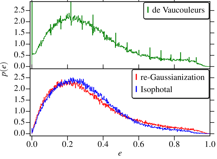
(a)

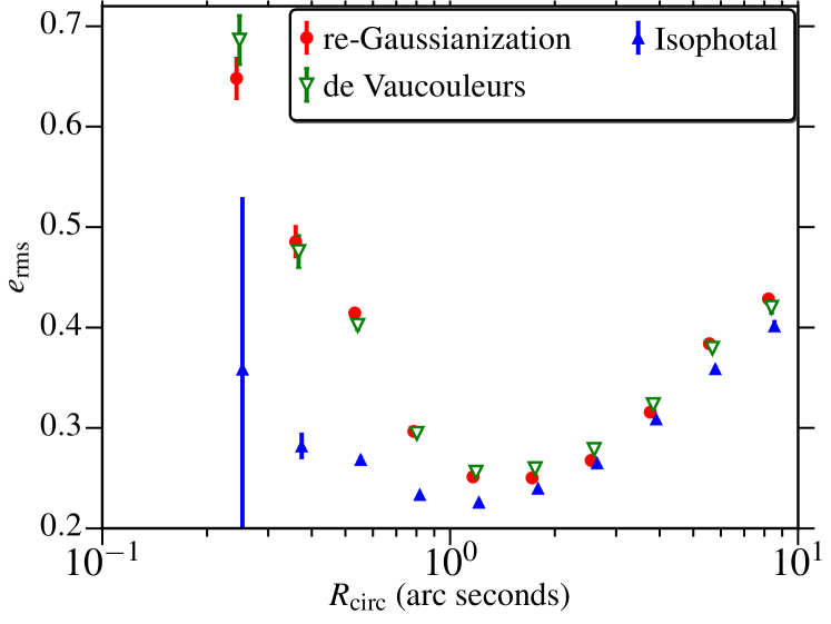
(b)

Figure 1: (a) Probability distribution of $e$ for different shape measurement methods. The periodic spikes in the de Vaucouleurs $p(e)$ are discussed in the text of Sec. 4.1. (b) The RMS ellipticity per shape component, $e_{\text{rms}}$, for different shape measurement methods as a function of circularized apparent radius $R_{\text{circ}}$ (Eq. 23).

The lower values of $e_{\text{rms}}$ in isophotal shapes is primarily driven by the deficit of galaxies with $e>0.7$, as shown in Fig. 1(a). This could also be due to some systematic effect such as multiplicative bias from the PSF, which tends to make galaxy shapes rounder and will be more important for more elongated galaxies. The trends in $e_{\text{rms}}$ in Fig. 1(b) are consistent with the presence of some systematic bias. The PSF effects become more important for smaller galaxies (smaller $R_{\text{circ}}$), thus making them appear rounder and thereby reducing the incidence of high-ellipticity objects. The fact that the isophotal shapes, which have no PSF correction at all, have a lower $e_{\mathrm{rms}}$ and that this difference between isophotal and other shapes gets progressively more pronounced for galaxies with a small apparent size is a clear signature of PSF dilution systematics. Note that (for a fixed total flux), the effect of pixel noise increases measurement errors preferentially for the smaller sizes, leading to an increase in the $e_{\mathrm{rms}}$ for smaller galaxies for all measurement methods. While we have attempted to subtract the measurement errors, these are known to be underestimated (Reyes et al., 2012) and thus incompletely removed. Fully disentangling true physical effects like ellipticity gradients from systematic effects requires detailed analysis of different shape measurements using simulations, which is beyond the scope of this work. Our statements about radial evolution in ellipticity using isophotal shapes are only valid under the assumption that they are not significantly biased by the PSF or other systematics. In the context of the discussion so far, this is a reasonable assumption since $\sim 90\%$ of galaxies in our sample have $R_{\text{circ}}>1\arcsec$.

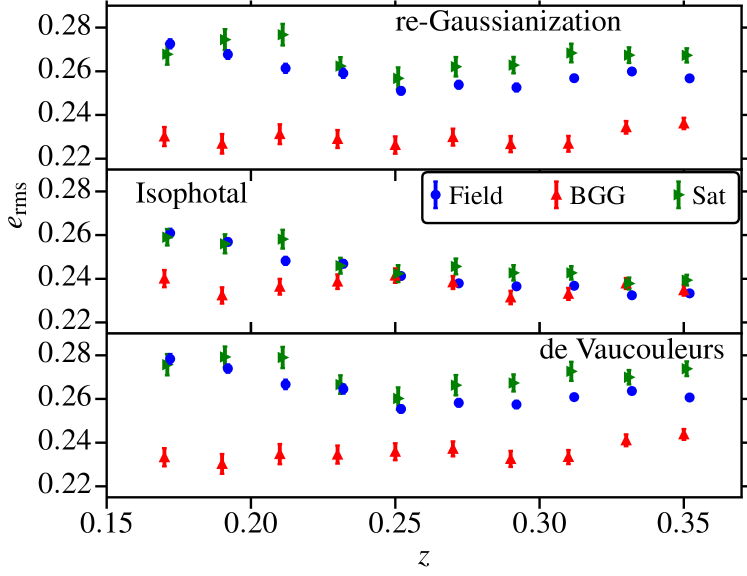
(a)

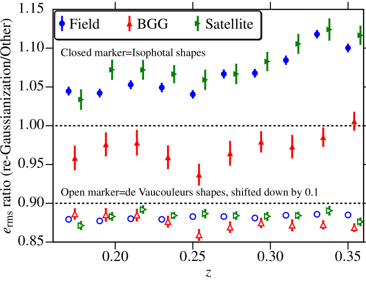
(b)

Figure 2: (a) The $e_{\text{rms}}$ as a function of redshift for galaxies in different environments using different shape measurement methods. BGGs are rounder than satellite and field galaxies using all three methods, though the differences are much less significant using isophotal shapes. (b) Ratio of $e_{\text{rms}}$ using re-Gaussianization shape to isophotal or de Vaucouleurs shapes for galaxies in different environments. BGGs are relatively more elliptical in isophotal shapes while satellites and field galaxies are more round using isophotal shapes. The differences are dominated by ellipticity differences using re-Gaussianization shapes as shown in (a). The variations in ellipticity between re- Gaussianization and de Vaucouleurs shapes are nearly identical across all galaxy environments (open markers in (b)).

As described in Sec. 3.3.6, few studies have observed the ellipticity trends in small samples of elliptical galaxies (see for eg. di Tullio, 1978, 1979; Pasquali et al., 2006). di Tullio (1978, 1979) first identified environment dependence of ellipticity gradients. Galaxies that have increasing ellipticity with radius are found preferentially in dense environments like clusters and groups, while those that have decreasing ellipticity with radius were generally isolated though they were also found in groups. We study these trends in the much larger LOWZ sample by identifying BGGs, satellites and field galaxies. Fig. 2(a) shows the $e_{\text{rms}}$ for these different environment subsamples for all three shape measurements, and Fig. 2(b) shows the ratio of $e_{\text{rms}}$ from re-Gaussianization shapes to isophotal and de Vaucouleurs shapes as a function of redshift. For both re-Gaussianization and de Vaucouleurs shapes, BGGs are rounder than field and satellites galaxies, while the trend is less clear for isophotal shapes. Doing the comparison between different shapes as shown in Fig. 2(b), BGGs get more elliptical with increasing radius while satellites and field galaxies get rounder, consistent with the observations of di Tullio (1979).

4.2 Systematics in two-point functions

In this section we show some systematics tests in the intrinsic alignment two-point correlation functions. Fig. 3 shows the density-shape ($w_{g+}$) and shape-shape ($w_{++}$) correlations using large $\Pi$ separations ($|\Pi|\in[200,500]$ $h^{-1}\text{Mpc}$). For such large separations, we do not expect any contribution from intrinsic alignments, so a deviation of the signals from zero is more likely from additive systematics due to the PSF (in the case of $w_{++}$) or, on small scales, incorrect sky subtraction. These signals are mostly consistent with zero (see Table 1 for $\chi^{2}$ and $p$ values) and thus do not indicate the presence of systematics, except for $w_{++}$ with de Vaucouleurs shapes on large scales. The slight negative signals in $w_{g+}$ are consistent in magnitude and $r_{p}$-scaling with the presence of a small lensing signal (tangential shape alignments) given the redshift separations between the galaxy pairs and the known lensing signals from Paper I.

Correlation	Shape	$\chi^{2}$	$p-$value
$w_{g+}$	re-Gaussianization	17.9	0.29
$w_{g+}$	Isophotal	17.4	0.31
$w_{g+}$	de Vaucouleurs	20.4	0.19
$w_{++}$	re-Gaussianization	9.8	0.79
$w_{++}$	Isophotal	15.2	0.43
$w_{++}$	de Vaucouleurs	31.6	0.02

Table 1: $\chi^{2}$ and $p-$values for $w_{g+}$ and $w_{++}$ calculated using large $\Pi$ separations ($|\Pi|\in[200,500]$ $h^{-1}\text{Mpc}$) and different shape measurements. All signal are consistent with a null detection except for $w_{++}$ with de Vaucouleurs shapes.

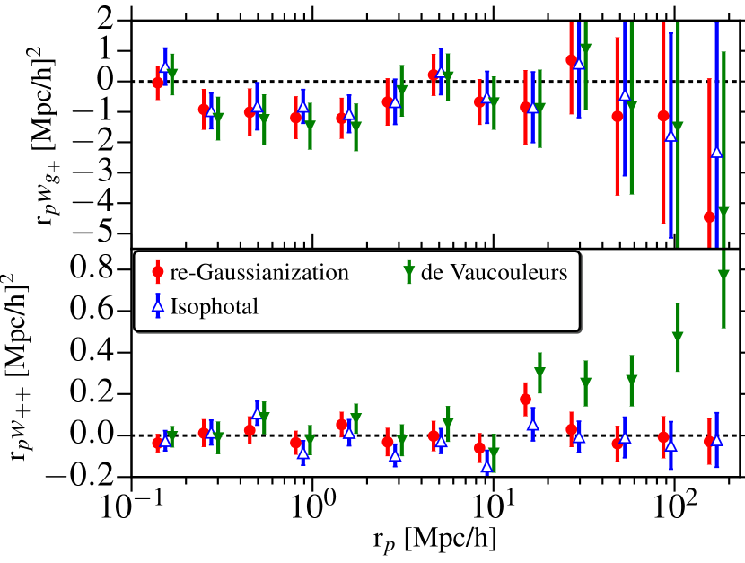
Figure 3: Intrinsic alignment correlation functions using integration only over large line-of-sight separations ($|\Pi|\in[200,500]$$h^{-1}\text{Mpc}$) for the full LOWZ sample, with different shape measurement methods. The top and bottom show $r_{p}w_{g+}$ and $r_{p}w_{++}$, respectively.

As discussed in Sec. 3.3.5, additive PSF contamination in galaxy shape measurements can affect IA results, particularly $w_{++}$, if not corrected properly. To better understand this contamination, we directly calculate $\langle\gamma_{\text{obs}}\gamma_{\text{PSF}}\rangle$ cross-correlations using PSF shapes at the positions of galaxies. Fig. 4 shows the cross-correlations of different shape measurements with the PSF shape, $w_{++}^{\text{sys}}$, with de Vaucouleurs shapes showing strong correlations. These are likely the cause of the non-zero $w_{++}$ for large $\Pi$ in Fig. 3. Isophotal and re-Gaussianization shapes, on the other hand, show much lower levels of contamination, which suggests that these two are not strongly affected by additive PSF errors. Fig. 5 shows $A_{\text{PSF}}$ defined in Eq. (26) for different galaxy subsamples and shape measurement methods. This figure confirms our conclusion that de Vaucouleurs shapes have stronger additive PSF bias while isophotal and re-Gaussianization shapes have much smaller levels of contamination. Using the full LOWZ sample, we find $A_{\text{PSF}}=-0.019\pm 0.015$, $-0.049\pm 0.017$, and $-0.29\pm 0.02$ for re-Gaussianization, isophotal, and de Vaucouleurs shapes. Our value of $|A_{\text{PSF}}|$ for re-Gaussianization is smaller than that in Mandelbaum et al. (2015), who found $A_{\text{PSF}}\sim-0.1$; however, those results were for a simulated galaxy sample extending to much lower $S/N$ and resolution, which is expected to have relatively stronger additive systematics compared to LOWZ.

It is quite interesting and somewhat counter-intuitive that the de Vaucouleurs shapes, which include PSF correction with an approximate PSF model, have a much larger $A_{\text{PSF}}$ than the isophotal shapes, which do not. We propose that the reason for this is that the de Vaucouleurs shapes are weighted towards the central part of the galaxy light profile and thus rely on small scales (which are highly sensitive to the PSF). Thus, a small error in the PSF model can be very important. In contrast, the isophotal shapes use such a low surface-brightness isophote that they correspond to much larger scales, where the impact of the PSF is much smaller, and even without correction, $A_{\text{PSF}}$ can be quite small.

There is no strong dependence of the additive PSF contamination on galaxy properties such as luminosity and color. The contamination in de Vaucouleurs shapes does show significant redshift dependence, with the higher redshift sample, Z2, showing stronger contamination; a similar but much less significant effect is present in isophotal and re-Gaussianization shapes. This is likely due the fact that higher redshift galaxies have a smaller apparent size, making the contamination from PSF anisotropy more important for such galaxies. There are hints of luminosity dependence to the additive PSF contamination for both de Vaucouleurs and isophotal shapes, though these trends are not very significant. $|A_{\text{PSF}}|$ is expected to be larger for lower luminosity samples since those galaxies generally have smaller apparent size, making PSF contamination more important.

We caution that the tests in this section do not rule out multiplicative bias, which could change the IA two-point correlation functions in a way that is degenerate with the IA amplitude $A_{I}$.

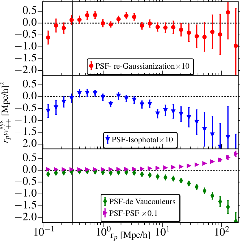
Figure 4: Galaxy shape vs. PSF shape cross-correlations using the full LOWZ sample with different shape measurement methods, as a way to reveal additive PSF contamination in the galaxy shapes. The signal for re-Gaussianization and isophotal shapes has been multiplied by a factor of 10 in this plot, while the signal for PSF-PSF correlations is suppressed by a factor of 10. The black solid line marks the SDSS fiber collision limit.

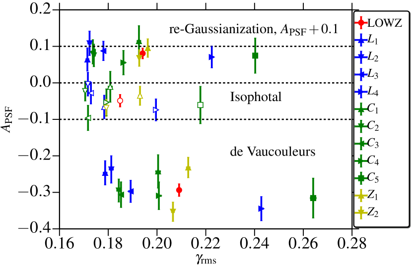
Figure 5: Galaxy shape vs. PSF shape cross-correlation amplitude, $A_{\text{PSF}}$ (Eq. 26), using isophotal (open markers), re-Gaussianization (filled markers, $A_{\text{PSF}}+0.1>0$, shifted up for clarity) and de Vaucouleurs (filled markers, $A_{\text{PSF}}<-0.1$) shapes. re-Gaussianization and isophotal shapes show relatively low and similar amplitudes while de Vaucouleurs shapes have a large value of $A_{\text{PSF}}$, indicative of significant additive bias from the PSF anisotropy.

4.3 Ellipticity definition

To confirm the consistency of intrinsic alignments results using the two different ellipticity definitions in Eq. (17) and (20), we calculate the density-shape correlation function $w_{g+}$ with isophotal and de Vaucouleurs shapes using both definitions, modifying the $w_{g+}$ estimator appropriately. Fig. 6 shows the ratio of the inferred $A_{I}$ for different subsamples from the NLA model fits to $w_{g+}$ using the two shear estimators. $A_{I}$ measured using both definitions are consistent within 1$\sigma$ for isophotal shapes, and there are no strong dependences on galaxy properties such as color or luminosity. In principle, this is precisely as expected; however, differences could arise due to systematic errors in the RMS ellipticity calculation if the error estimates are incorrect. For the rest of the paper, we use $\varepsilon$ (Eq. 20) as our galaxy shape estimator for isophotal and de Vaucouleurs shapes.

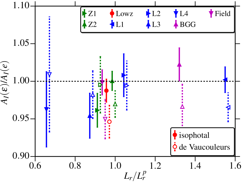
Figure 6: Ratio of IA amplitude, $A_{I}$, obtained via NLA model fits to $w_{g+}$ calculated using shears from two different ellipticity definitions, $e$ (Eq. 17) and $\varepsilon$ (Eq. 20), for isophotal (solid lines) and de Vaucouleurs (dashed lines) shapes. Both definitions give consistent results across all luminosities, redshifts, and environments.

4.4 IA with different shape measurements

In this section we present the IA measurements using the different shape measurement methods discussed in Sec. 3.3.

Fig. 7(a) shows the $w_{g+}$ measurement for the full LOWZ sample using all three shape measurement methods. Isophotal shapes give the highest IA amplitude, followed by de Vaucouleurs and re-Gaussianization shapes. Fig. 8 shows the amplitude trends more clearly, where we have plotted the ratio of $A_{I}$ for isophotal and de Vaucouleurs shapes with respect to re-Gaussianization shapes, for various subsamples defined by different galaxy properties. Isophotal (de Vaucouleurs) shapes give a higher $A_{I}$ by $\sim 40\%~{}(20\%)$ compared to re-Gaussianization shapes, with no clear trends with galaxy properties like luminosity, color, and redshift.

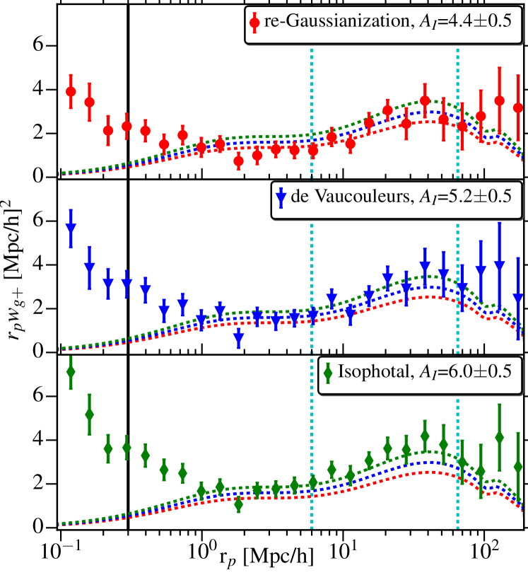
(a)

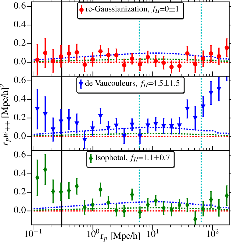
(b)

Figure 7: (a) The projected galaxy density-shape correlation function $w_{g+}$ (Eq. 9) using the full LOWZ sample and different shape measurement methods, isophotal (blue), re-Gaussianization (red) and de Vaucouleurs shapes (green), along with the best-fitting NLA models. For comparison, the best-fitting NLA models for all three shape measurement methods are plotted on all panels. Isophotal shapes show the highest IA signal, followed by de Vaucouleurs and re-Gaussianization shapes (note that error bars are correlated between the different shape measurement methods). The solid black line shows the SDSS fiber collision limit, and the dashed cyan lines show the range of $r_{p}$ used for the NLA model fitting. (b) Same as (a), but for the projected shape-shape correlation function $w_{++}$ (Eq. 10).

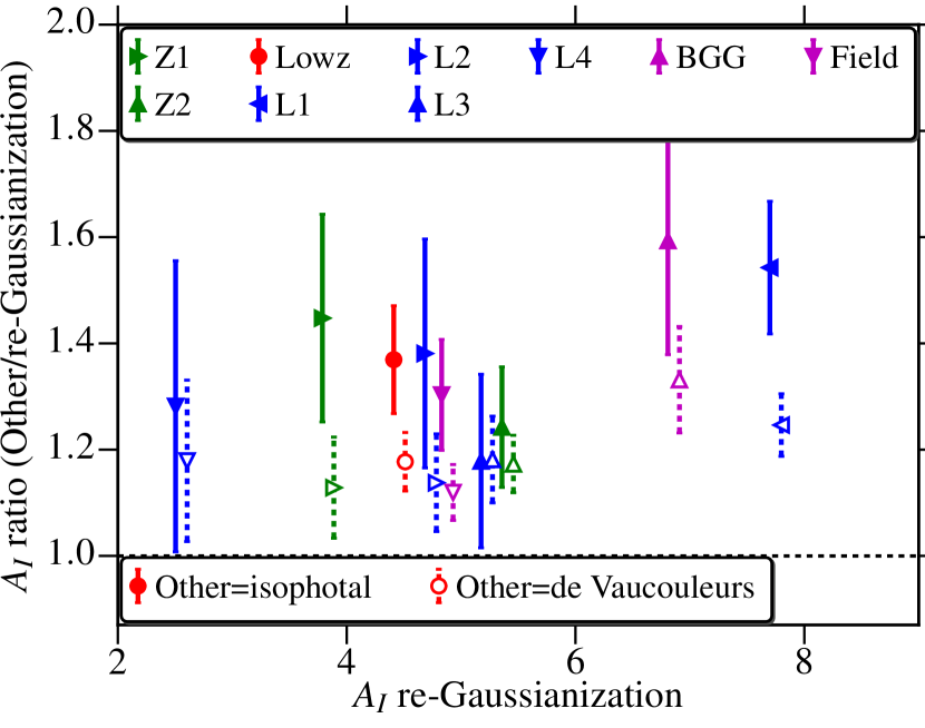
Figure 8: Comparison of NLA model amplitude $A_{I}$ for isophotal and de Vaucouleurs vs. re-Gaussianization shape measurements. Isophotal (de Vaucouleurs) shapes consistently give a higher amplitude by $\sim 40\%~{}(20\%)$ compared to re-Gaussianization shapes. The de Vaucouleurs results have been shifted horizontally for clarity.

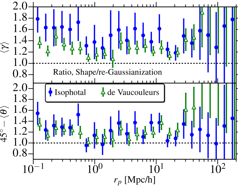
Figure 9: Ratio of mean intrinsic shear, $\langle\gamma\rangle$ (Eq. 27) and mean alignment angle, $45^{\circ}-\langle\theta\rangle$ (Eq. 28) using different shape measurement methods.

To further understand the effects of different shape measurement methods, we measure two more IA estimators, $\langle\gamma\rangle$ and $\langle\theta\rangle$, defined as

$$\langle\gamma\rangle=\frac{S_{+}D}{SD}$$ (27)

$$\langle\theta\rangle=\frac{\theta_{SD}}{SD}$$ (28)

Both $\langle\gamma\rangle$ and $\langle\theta\rangle$ are calculated in a single $\Pi$ bin with $\Pi\in[-100,100]h^{-1}\text{Mpc}$. In the absence of intrinsic alignments, $\langle\gamma\rangle=0$ and $\langle\theta\rangle=45^{\circ}$, while in presence of IA, $\langle\gamma\rangle>0$ and $\langle\theta\rangle<45^{\circ}$ Fig. 9 shows the ratio of $\langle\gamma\rangle$ and $45^{\circ}-\langle\theta\rangle$ measured using isophotal and de Vaucouleurs shapes with respect to re-Gaussianization shapes. $\langle\gamma\rangle$ is higher for isophotal shapes followed by de Vaucouleurs shapes, as expected from $w_{g+}$ results. $45^{\circ}-\langle\theta\rangle$ is also higher.

There are a few possible explanations for these differences in IA amplitudes with different shape measurement methods. The first possibility, as discussed in Sec. 3.3.5 and observed in Sec. 4.2, is a systematic error from incorrect PSF removal. Isophotal shapes are not corrected for the PSF, while de Vaucouleurs shapes are only approximately corrected. As shown in Sec. 4.2, we have a clear detection of additive PSF bias in de Vaucouleurs shapes, though isophotal and re-Gaussianization shapes have much lower levels of contamination. The additive bias should drop out of $w_{g+}$ calculations, under the assumption that it is not correlated with the positions of other galaxies ($\langle g\gamma_{\text{PSF}}\rangle\sim 0$ in Eq. 24). We have not ruled out the presence of multiplicative bias, which could cause an apparent change in $A_{I}$, but is extremely difficult to rule out using the data alone. However, the simplest possible interpretation of how multiplicative bias should affect these results is not valid: if multiplicative bias is responsible for the lower RMS ellipticities using isophotal shapes compared to other methods in Fig. 1(b), then $A_{I}$ should be the lowest using isophotal shapes, not the highest.

Another possibility as discussed in Sec. 3.3.6 is the presence of some physical effect such as isophote twisting and/or ellipticity gradients. Since $w_{g+}$ is an ellipticity-weighted measure of IA, gradients in the ellipticity can also lead to higher $w_{g+}$. However, as discussed in Sec. 4.1, isophotal shapes have lower $e_{\mathrm{rms}}$ than re-gaussianization and de Vaucouleurs shapes. This suggests that if the galaxies have the same large-scale alignments with the tidal field at all radii, but an ellipticity gradient that modifies $e_{\mathrm{rms}}$, then isophotal shapes should have lowest $w_{g+}$ amplitude, not the highest. Moreover, ellipticity gradients alone cannot explain a stronger alignment angle $\langle\theta\rangle$ for isophotal shapes, as shown in Fig. 9.

The other physical effect, isophote twisting, is related to the fact that outer regions of galaxies may be more susceptible to the local and large-scale tidal fields and thus show stronger alignments. If this effect is important, isophotal shapes should have the highest IA amplitude, followed by de Vaucouleurs and finally re-Gaussianization shapes, consistent with our results. The results in Fig. 9 are also consistent with this physical effect. Given that PSF-related systematics should cancel out of $\langle\theta\rangle$ (since the alignment is being calculated with respect to galaxy positions that are not aligned with respect to the PSF), and multiplicative biases also cannot modify the alignment angle, it is difficult to interpret that finding as anything other than isophote twisting.

Finally, Fig. 7(b) shows the shape-shape ($w_{++}$) correlation functions. The $w_{++}$ detection using isophotal and re- Gaussianization shapes is not very significant, and most of the signal using de Vaucouleurs shapes can be attributed to additive PSF bias as shown in Sec. 4.2. The detection significance of our isophotal measurements is not consistent with that of Blazek et al. (2011), who reported a high-significance detection of $w_{++}$ using measurements of Okumura et al. (2009) with isophotal shapes. While this could also be due to the differences in sample definition, our results in Paper I suggest that even with an appropriately bright subset of LOWZ, our results may not agree. Thus, we will address this discrepancy in greater detail in Sec. 4.6 after we have discussed the anisotropy of IA signals, which turns out to be an important factor in this difference.

4.5 Anisotropy of IA

As discussed in Sec. 2.3, IA measurements suffer from anisotropy in $(r_{p},\Pi)$ introduced by the projected shapes, which do not allow measurement of the IA signal along the line of sight. To enable a study of this effect, Fig. 10 shows $\xi_{gg}$, $\xi_{g+}$, and $\xi_{++}$ as a function of $r_{p}$ and $\Pi$, as well as the corresponding monopole and quadrupole measurements defined in Sec. 2.3. The top row shows the galaxy clustering measurements as well as the model predictions. Non-linear theory predictions with the Kaiser formula for RSD match the data for $r_{p}\gtrsim 5h^{-1}\text{Mpc}$ and $s\gtrsim 20h^{-1}\text{Mpc}$, though there are deviations below these scales due to nonlinear RSD and the Finger-of-God effect.

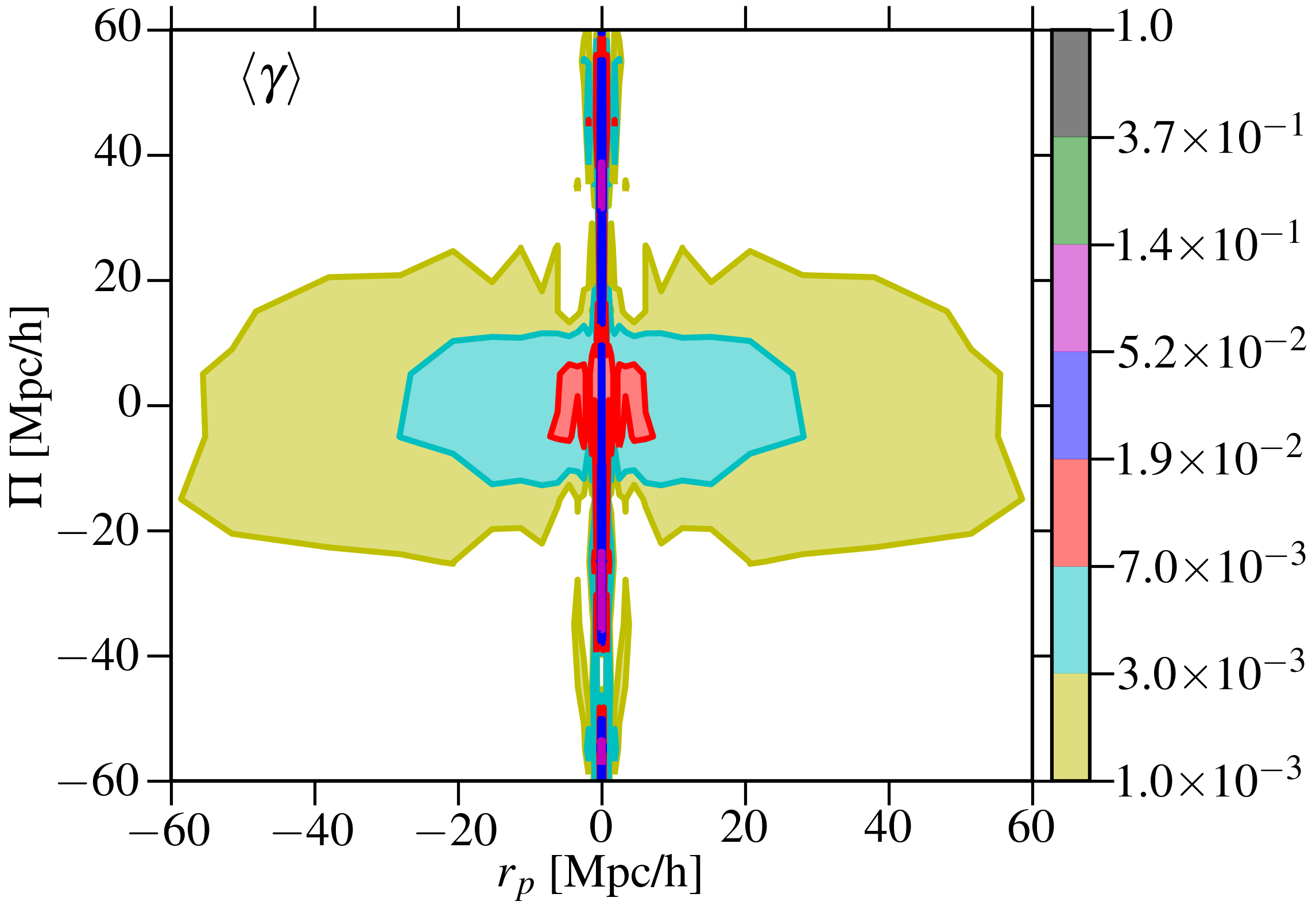
(a)

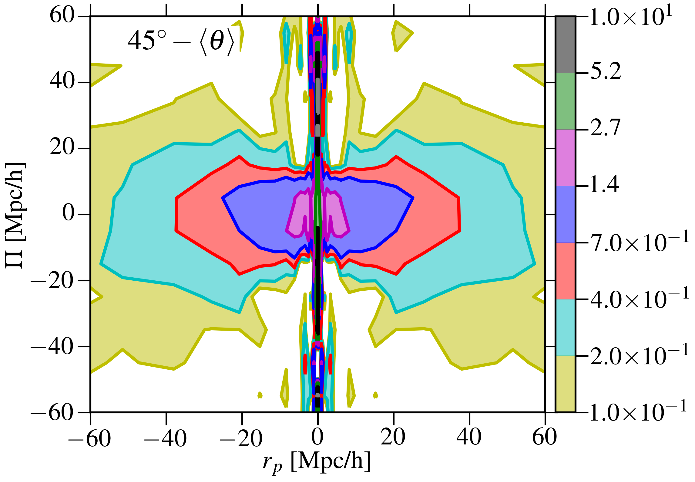
(b)

Figure 11: Similar to the left column of Fig. 10. (a) $\langle\gamma\rangle$ (Eq. 27) as a function of $r_{p},\Pi$. (b) $45^{\circ}-\langle\theta\rangle$ (Eq. 28) as a function of $r_{p},\Pi$. Both (a) and (b) use isophotal shapes and the same binning as in Fig. 10, but there are no theory curves on these plots.

The middle row in Fig. 10 shows $\xi_{g+}$ measurements using isophotal shapes. Again, the NLA model fits the data well for $r_{p}\gtrsim 5h^{-1}\text{Mpc}$ and $s\gtrsim 20h^{-1}\text{Mpc}$ with deviations at small scales due to nonlinear RSD and clustering. The strong anisotropy introduced by the projected shapes is clearly visible in the shape of the peanut-shaped contours, where the signal drops off quickly with $\Pi$. The NLA model incorporates this anisotropy and is consistent with the data. The redshift-space structure of $\langle\gamma\rangle$ and $\langle\theta\rangle$ (shown in Fig. 11) is very similar to that of $\xi_{g+}$.

The bottom row in Fig. 10 shows $\xi_{++}$ measurements using isophotal shapes. To display NLA model predictions, we use the best-fitting parameters from fitting $w_{g+}$, with $f_{II}=1$ (solid lines) and $f_{II}=2$ (dashed lines). The two-dimensional contours in Fig. 10(e) suggest that the data prefer the model with $f_{II}=2$. However, these contours are quite noisy, so Fig. 10(e) is not a reliable test of the validity of the model. In Fig. 10(f), we show a clear detection of the monopole for $\xi_{++}$, with the data again preferring a higher amplitude than predicted by NLA model ($f_{II}>1$). This discrepancy could either be from the effects of non-linear physics that is not included in the NLA model (Blazek et al., 2015), or from additive PSF contamination. Even though additive PSF contamination was shown to be low for isophotal shapes ($|A_{PSF}|\sim 0.05$), the contamination in $\xi_{++}$ could still be strong enough to increase the observed $\xi_{++}$ amplitude. In Fig. 12, we show the $\xi_{++}$ monopole for the full LOWZ sample and the brightest subsample, $L_{1}$, along with the predicted PSF contamination. For large scales, $s>30$$h^{-1}\text{Mpc}$, the PSF contamination alone can account for the observed $\xi_{++}$ signal for the full LOWZ sample. At smaller scales, the PSF effects are subdominant, which make it unlikely to be responsible for the higher than predicted amplitude. Both LOWZ and $L_{1}$ samples prefer a higher amplitude; based on $\Delta\chi^{2}$, the $p-$value$=0.01$ ($0.15$) for LOWZ ($L_{1}$). However, the $f_{II}=1$ model is not ruled out by either sample, with a $p$-value of $0.07$ ($0.44$) for LOWZ ($L_{1}$). With PSF effects being subdominant, we conclude that the discrepancy between NLA and data is primarily due to non-linear physics (e.g. non-linear clustering, non-linear RSD), which become important for scales $s<30h^{-1}\text{Mpc}$ and generally increase the amplitude (Blazek et al., 2015).

The $\xi_{++}$ quadrupole moment in both the data and the NLA model prediction is close to zero. $\xi_{++}$ is relatively more isotropic (Croft & Metzler, 2000) than $\xi_{g+}$ as some large-scale modes along the line-of-sight can introduce similar IA in projected galaxy shapes with larger separation along $\Pi$. These correlations show up in the shape-shape correlation function but not in the density-shape correlations. Mathematically, these terms are sourced by the $J_{0}$ term combined with $(1-\mu^{2})^{2}$ (see Eq. 14) which is more extended along $\Pi$, while the $J_{2}$ and $J_{4}$ terms are more extended along $r_{p}$. The combination of $J_{0}$ and $J_{4}$ terms makes $\xi_{++}$ relatively more isotropic than $\xi_{g+}$.

As a final exploration of the anisotropy of intrinsic alignments, Fig. 13 shows $\xi_{gg}$ and $\xi_{g+}$ measured using the MassiveBlack-II (MB-II) cosmological hydrodynamic simulation (Khandai et al., 2015) at $z=0.3$, along with NLA model predictions. The top row shows the signal without RSD, along with model predictions with $\beta=0$. Bottom row shows both signal and model with RSD effects included. The effects of RSD are clearly visible in $\xi_{gg}$. On the other hand, the variations in $\xi_{g+}$ from top to bottom row are far less pronounced, consistent with our findings that $\xi_{g+}$ is not affect by RSD to first order, $\beta_{\gamma}=0$ (see Paper I for derivation). Qualitatively, the simulation results produce the features seen in the data and show good agreement with the model within the limitations of validity of the model (which does not include nonlinear RSD or nonlinear galaxy bias, resulting in small-scale discrepancies). At large scales ($r\gtrsim 20h^{-1}\text{Mpc}$) cosmic variance plays an important role due to the limited size of the simulation box ($100h^{-1}\text{Mpc}$), making it difficult to compare the model and simulation data at these scales.

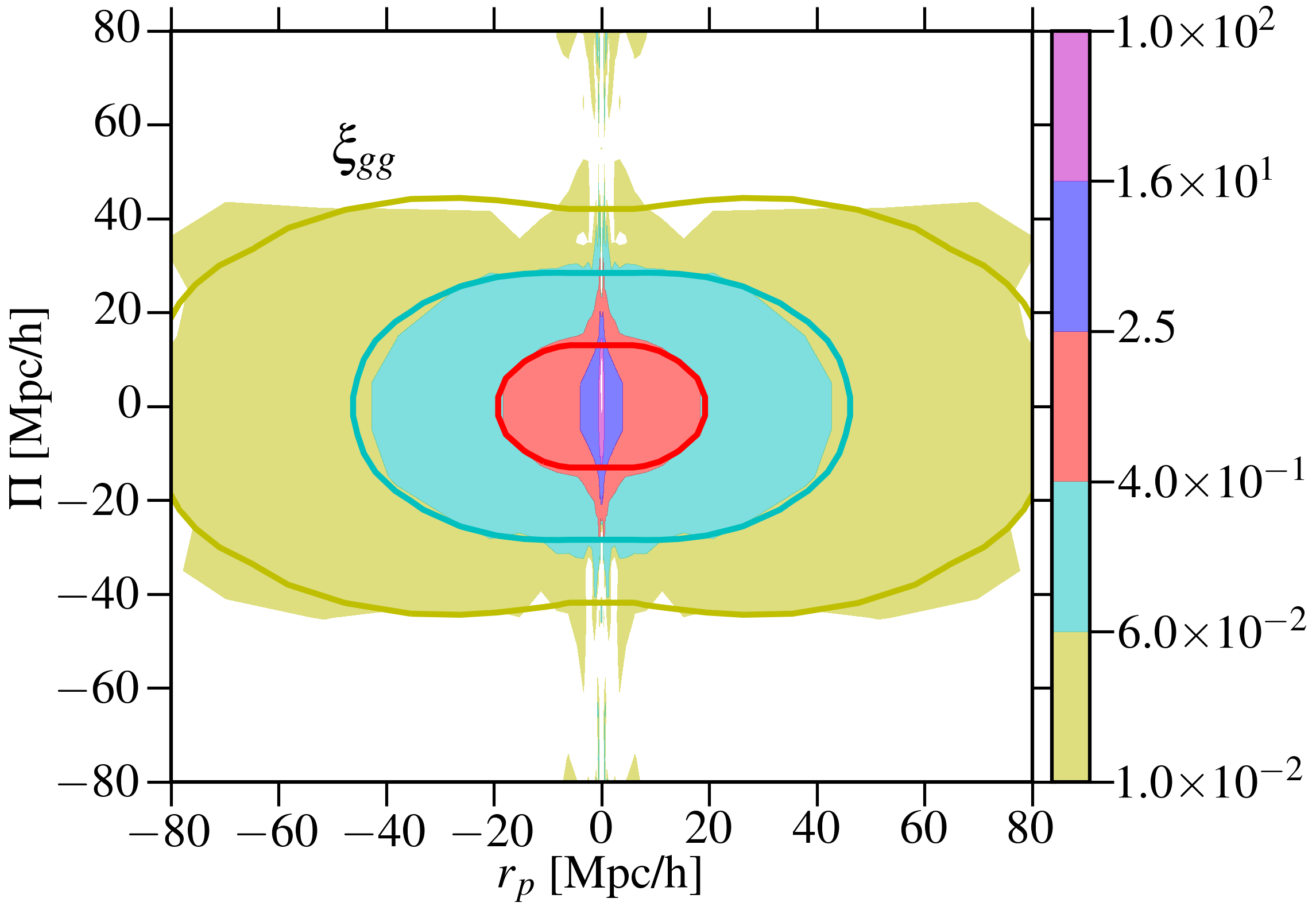
(a)

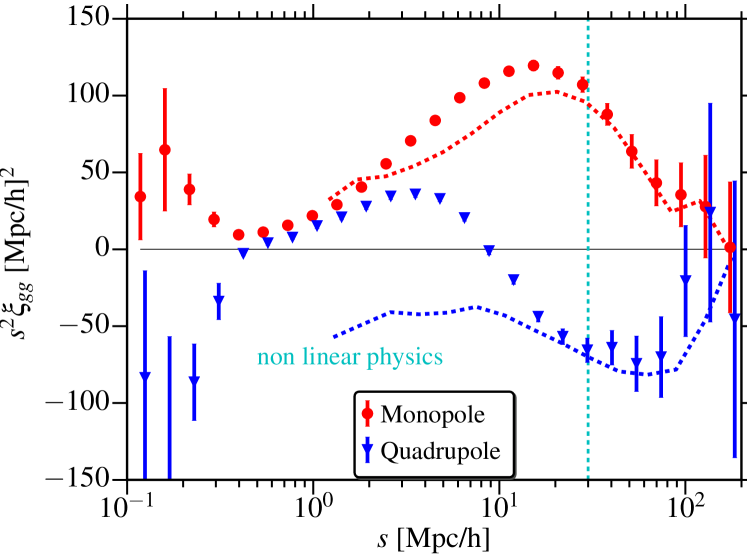
(b)

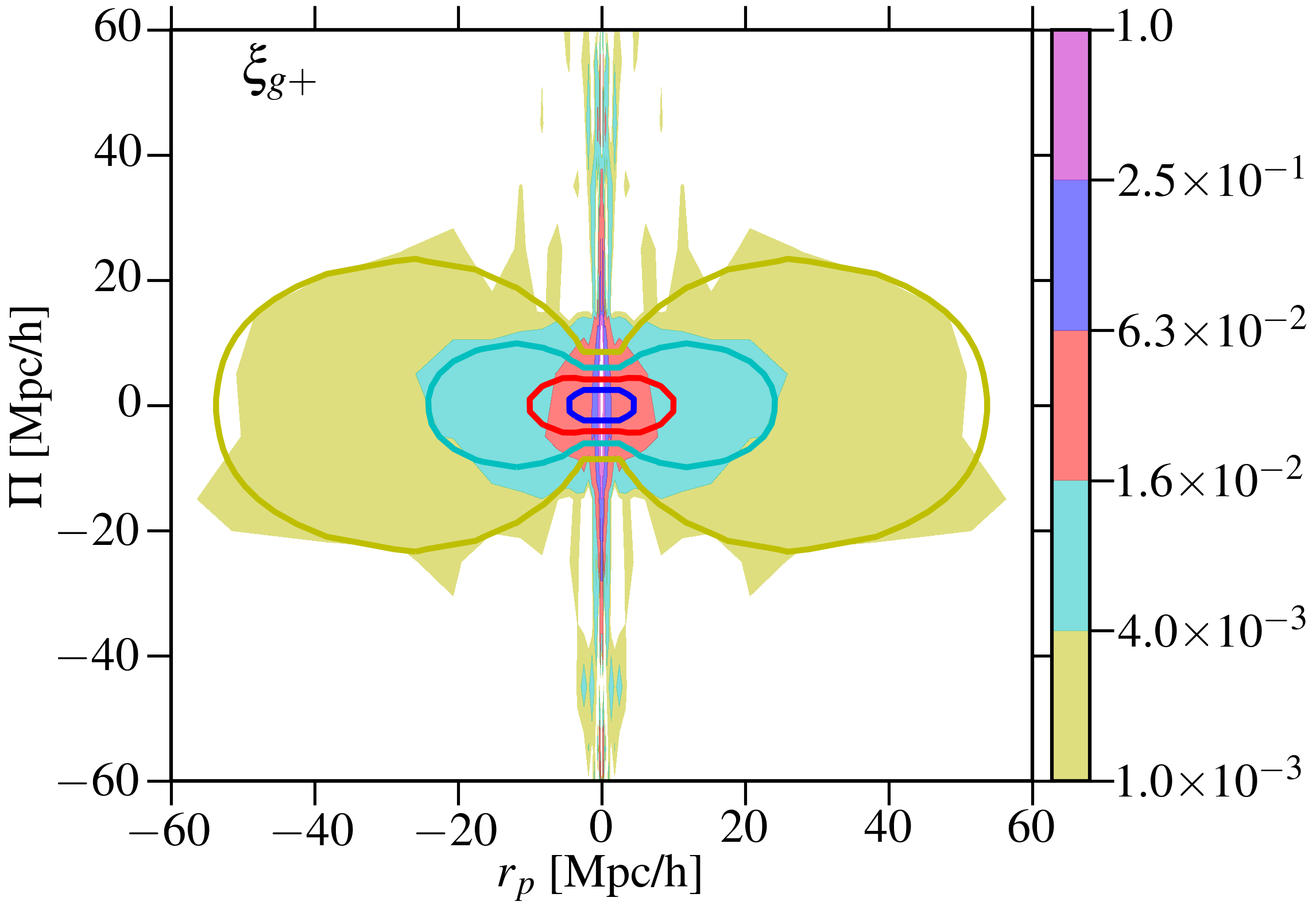
(c)

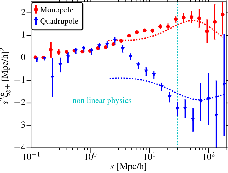
(d)

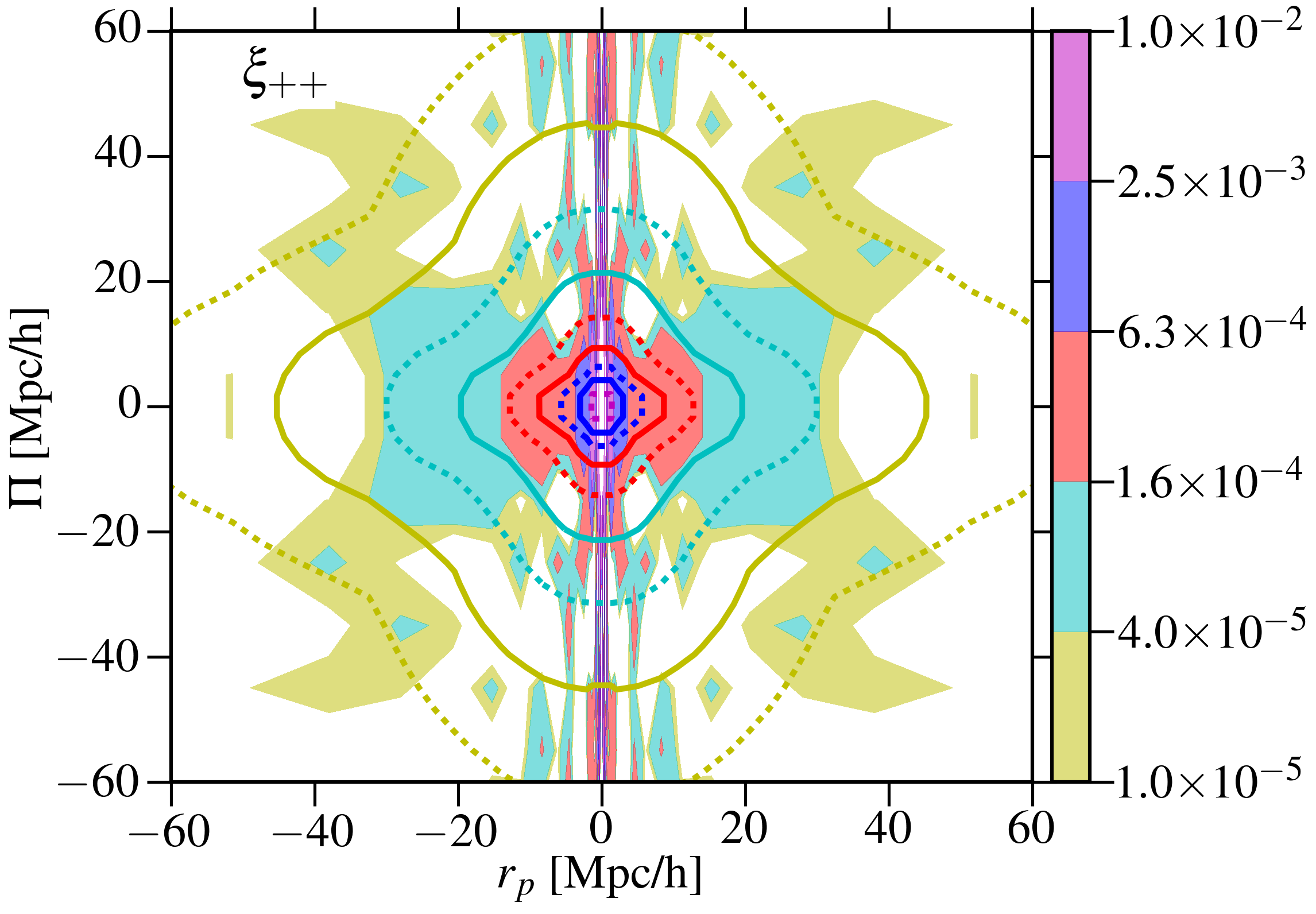
(e)

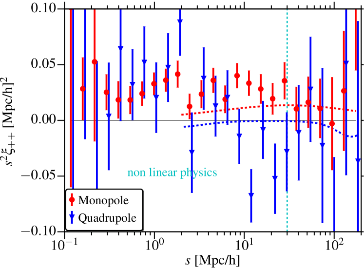
(f)

Figure 10: The 3D galaxy-galaxy correlation function $\xi_{gg}$ (top row, Eq. 12), galaxy density-shape correlation function $\xi_{g+}$ (middle row, Eq. 13) and shape-shape correlation function $\xi_{++}$ (bottom row, Eq. 14) as a function of $r_{p},\Pi$ (left column, reflected about $r_{p}=0$) and their multipole moments (right column). All plots use isophotal shapes. In the left column, the filled contours are showing the data, while solid lines are the theory predictions corresponding to the outer edge of the filled contours. The right column shows monopole and quadrupole measurements as a function of three dimensional redshift space separation ($s=\sqrt{r_{p}^{2}+\Pi^{2}}$ [Mpc$/h$]). The points are measurements from the data, while dashed lines are NLA model predictions. Theory predictions in both columns are from the best-fitting models to $w_{gg}$ and $w_{g+}$, with $f_{II}=1$ in $\xi_{++}$. The dashed lines in (e) show predictions with $f_{II}=2$. The linear models with non-linear power spectrum are consistent with data for $s\gtrsim 30~{}h^{-1}\text{Mpc}$, below which significant deviations are expected due to non-linear RSD and, on even smaller scales, non-linear galaxy bias.

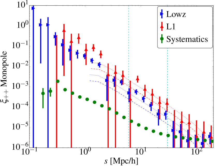
Figure 12: The 3D shape-shape correlation function $\xi_{++}$ (Eq. 14) monopole moment using isophotal shapes for LOWZ (blue) and the $L_{1}$ (red) subsample, along with theory predictions from the best-fitting NLA model to $w_{g+}$ with $f_{II}=1$ (dashed lines) and $f_{II}=2$ (dotted lines). Green points also show the monopole of the expected additive PSF contamination based on the analysis in Sec. 4.2, $\xi_{++}^{\text{sys}}\approx A_{\text{PSF,isoph}}^{2}\times\xi_{++}^{\text{PSF-PSF}}$. Vertical lines at $s=6$ and $30h^{-1}\text{Mpc}$ show the limits used to calculate $\chi^{2}$ values to assess the goodness of the model.

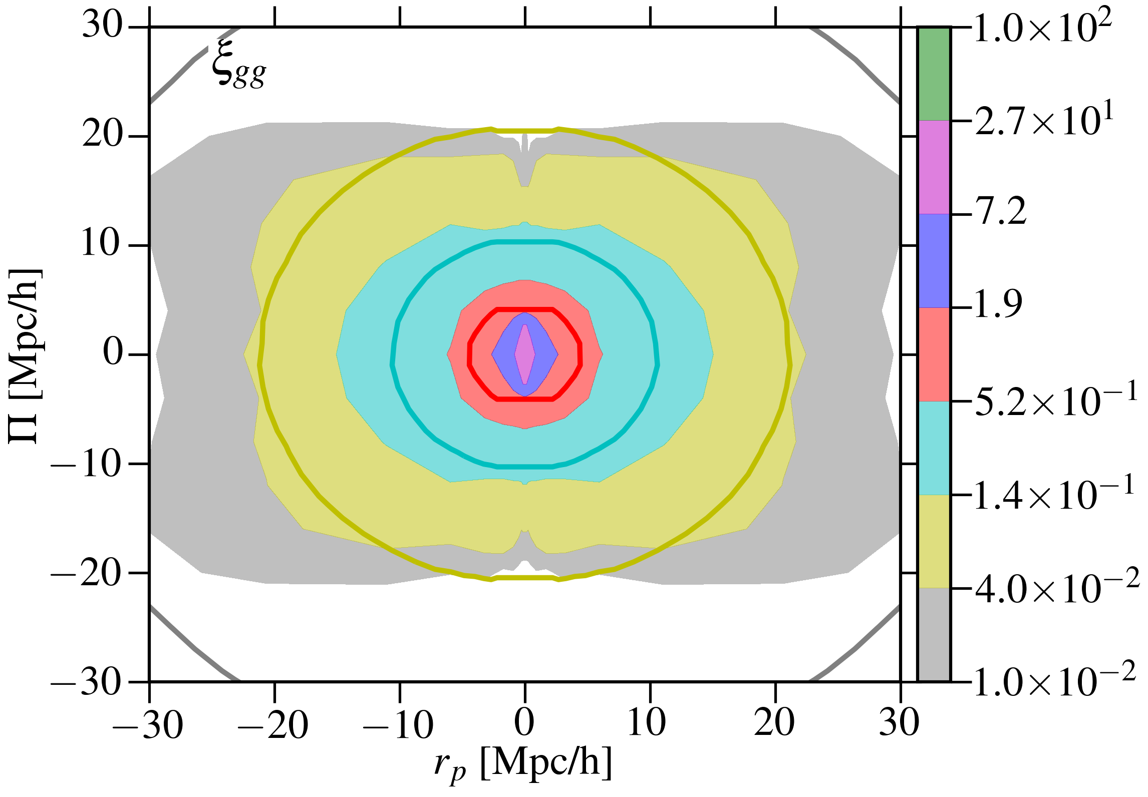
(a)

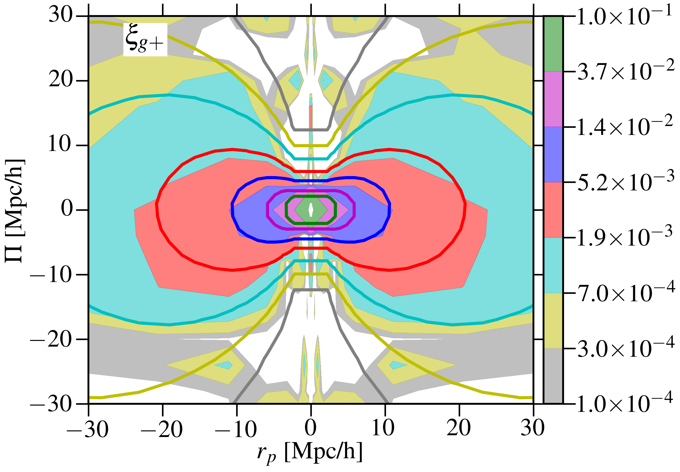
(b)

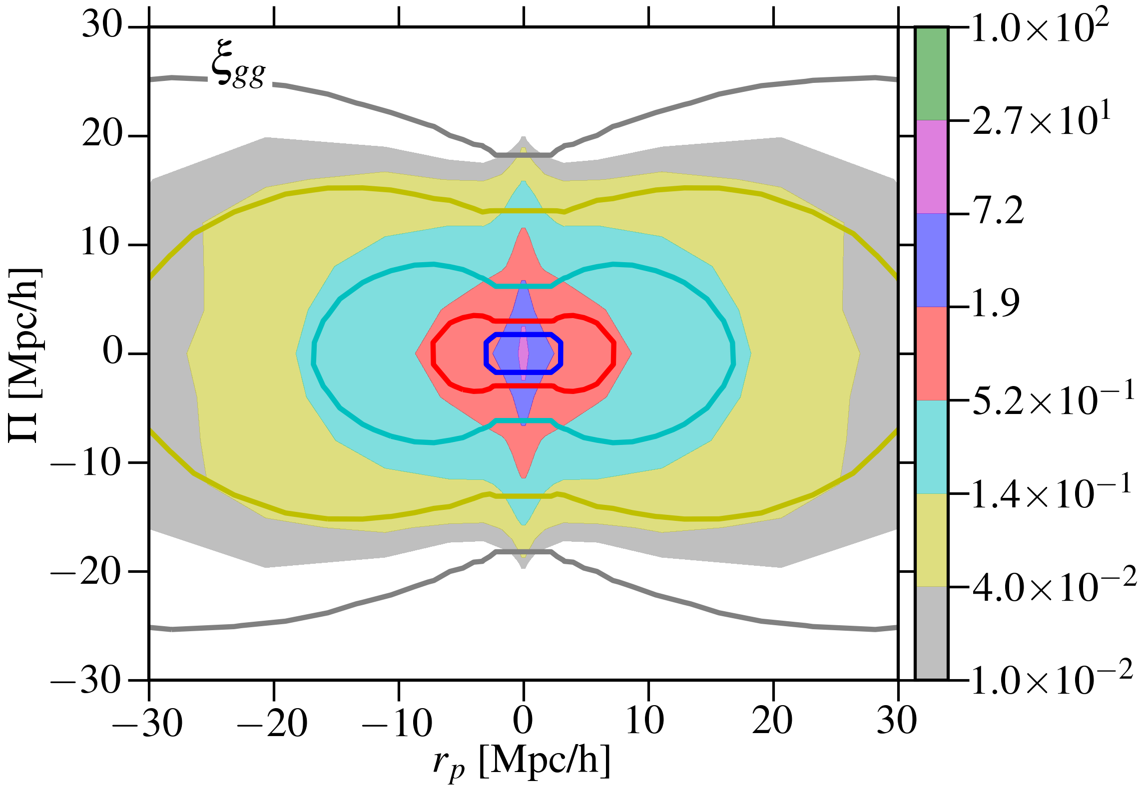
(c)

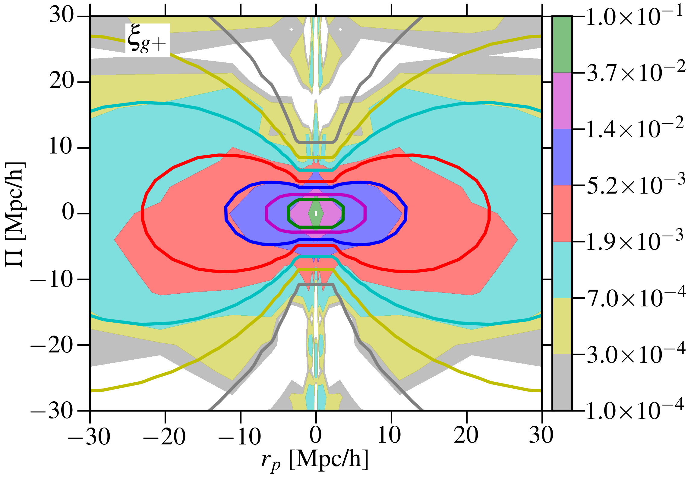
(d)

Figure 13: The 3D galaxy-galaxy correlation function $\xi_{gg}$ (Eq. 12) and galaxy density-shape correlation function $\xi_{g+}$ (Eq. 13) contour plots from the MB-II simulation, similar to Fig. 10(a) and Fig. 10(c). The top row shows the signal and model without RSD, while the bottom row includes RSD. We used linear bias $b=0.8$ and $A_{I}=6$ for the theory predictions. Note that the small scale behavior in (a,b) is an artifact from binning, with logarithmic bins in $r_{p}$ and linear bins in $\Pi$ with $d\Pi=5h^{-1}\text{Mpc}$.

4.6 Comparison with other studies

As discussed in Paper I and Sec. 4.4, there is an apparent discrepancy in detection significance of our $w_{++}$ measurements with those of Blazek et al. (2011). Blazek et al. (2011) used a projection of 3D results from Okumura et al. (2009), who measured $\xi_{++}$ ($C_{11}$ in their notation) as function of redshift-space separation $s$ using isophotal shapes. We hereafter use $C_{11}$ to refer to $\xi_{++}(s)$, to distinguish it from our measurement of $\xi_{++}(r_{p},\Pi)$. Assuming isotropy of $\xi_{++}(s)$, Blazek et al. (2011) projected the $C_{11}$ measurement onto $(r_{p},\Pi)$ space in order to calculate $w_{++}$. Their error estimates were based on generating 1000 random realizations of $C_{11}$, assuming Gaussian and independent errors. To test whether any parts of this procedure (either the signal or error estimation) could lead to differences in the estimated $S/N$ compared to our procedure, we repeat their analysis for our LOWZ sample, using isophotal shapes.

Fig. 14 shows our measurement of $C_{11}(s)$. With isophotal shapes, we have a significant detection of shape-shape correlations (as do Okumura et al. 2009 for LRGs), whereas the detection is not significant using re-Gaussianization shapes. We do not attempt a quantitative comparison with their results, since differences in sample selection complicate the comparison.

Using this $C_{11}(s)$ measurement with isophotal shapes, we repeat the procedure of Blazek et al. (2011) to get $w_{++}(r_{p})$. We project the $C_{11}$ measurement onto the $(r_{p},\Pi)$ plane, using 200 $\Pi$ bins with $\Pi\in[-100,100]h^{-1}\text{Mpc}$ and $d\Pi=1h^{-1}\text{Mpc}$. Fig. 15 compares the $w_{++}$ obtained using different methods. The $w_{++}$ for the LOWZ sample calculated using the Blazek et al. (2011) method of projecting $C_{11}(s)$ does have a higher detection significance compared to the $w_{++}$ using our $\xi_{++}(r_{p},\Pi)$ projection. This result is most likely due to the fact that $C_{11}$ is effectively the monopole term, which we detect with high significance (Fig. 10(f)). $C_{11}$ and the monopole have different amplitudes due to an additional $(2l+1)/2$ factor in the multipole moments (see Eq. 16). The differences in $S/N$ between $C_{11}$ and $w_{++}$ primarily come from the different sensitivity of the two estimators to the large $\Pi$ regions that contribute little signal but significant noise. In accordance with this explanation, we find that using $\Pi_{\text{max}}\sim 30h^{-1}\text{Mpc}$ when computing $w_{++}$ does give a statistically significant measurement (not shown). To compare error estimates, we repeat the Blazek et al. (2011) analysis but obtain errors using 100 jackknife regions instead of using 1000 random realizations of $C_{11}(s)$. The errors obtained using both methods are consistent. Note that since the LRG sample used by Okumura et al. (2009) is brighter than the LOWZ sample, the amplitude for the Blazek et al. (2011) $w_{++}$ measurement is expected to be higher than for LOWZ. Also, the choice of $d\Pi=1~{}h^{-1}\text{Mpc}$ leads to an approximately constant $w_{++}$ for $r_{p}<1h^{-1}\text{Mpc}$ since all bins are dominated by $C_{11}$ values from $s\sim 1h^{-1}\text{Mpc}$, given that the signal drops exponentially with increasing $s$ and bins with large $\Pi$ do not contribute much. Hence, the apparently constant $w_{++}$ at $r_{p}<1h^{-1}\text{Mpc}$ in Fig. 15 is not physical.

In Fig. 15 we also show the theory prediction from the best-fitting NLA model to $w_{g+}$. As in Fig. 12, the data prefer a higher amplitude than predicted by the NLA model, likely due to the effects of non-linear physics beyond the NLA model. This result is inconsistent with the findings of Blazek et al. (2011), who found consistent IA amplitudes from both $w_{g+}$ and $w_{++}$. Their sample, however, is similar to our $L_{1}$ sample, which as shown in Fig. 12 is consistent with $f_{II}=1$.

To summarize, we have investigated three possible reasons for the apparent difference in $w_{++}$ detection significance in Blazek et al. (2011) compared to Paper I. We find that the primary causes are (a) use of isophotal rather than re-Gaussianization shapes (increased signal), and (b) the projection of $C_{11}(s)$ rather than $\xi_{++}(r_{p},\Pi)$ (which ignores noisy higher multipoles), but conclude that their error estimate procedure is in agreement with the jackknife procedure. Hence the different $S/N$ in $w_{++}$ arises from differences in signal estimation (the first of which increases the signal, the second of which lowers the noise).

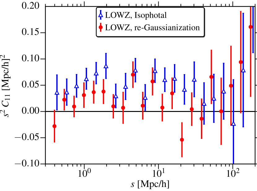
Figure 14: The 3D shape-shape correlation function as a function of redshift-space separation $s$, $C_{11}(s)$ (or $\xi_{++}(s)$), for the entire LOWZ sample, using re-Gaussianization and isophotal shapes.

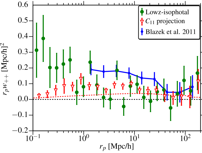
Figure 15: Comparison of $w_{++}$ measured in different ways. The green points show the signal after measuring $\xi_{++}$ in $(r_{p},\Pi)$ space and projecting along $\Pi$ using our standard methodology, while the red points show the signal obtained by projecting $C_{11}(s)$ following the approach of Blazek et al. (2011). The flatness of $w_{++}$ using the second approach at $r_{p}\lesssim 1h^{-1}\text{Mpc}$ is due to the choice of bin sizes ($d\Pi=1h^{-1}\text{Mpc}$); see text for details. The signal for brighter LRGs from Blazek et al. (2011) signal is plotted in green for reference, but should not be compared in detail with our results due to differences in sample definition.

Several other studies have used de Vaucouleurs and isophotal shapes to measure IA using the bright, nearby SDSS Main sample and the fainter, more distant BOSS CMASS samples (Hao et al., 2011; Li et al., 2013; Zhang et al., 2013). These samples have different redshifts and galaxy properties compared to LOWZ. As a result, the galaxy detection have different $S/N$ and resolution compared to the PSF, which should modify the observational systematics in galaxy shapes. Thus, our results about differences in systematics and in the IA amplitude using these different shape measurement methods cannot be used to make definitive statements about systematic effects in those studies.

5 Conclusions

In this work, we have studied SDSS-III BOSS LOWZ galaxy shapes and intrinsic alignments using three different shape measurement methods: re-Gaussianization (PSF-corrected, weighted towards inner regions of galaxies), isophotal (based on the shape of a low surface brightness isophote at large radius, not PSF-corrected), and de Vaucouleurs shapes (from fitting a de Vaucouleurs model to the light profile using an approximate PSF model, using a grid-based procedure that results in some quantization of model parameters). Different shape measurement methods give a different ellipticity for galaxies, which in the absence of systematic error implies a radial gradient in the galaxy shapes, with the shapes becoming rounder on average at large radius. These variations in ellipticity seem to depend on the galaxy environment, with brightest group galaxies (BGGs) actually becoming more elliptical with radius but satellites and field galaxies becoming rounder. The overall sign of the ellipticity gradients is consistent with hydrodynamic simulations (Tenneti et al., 2015) and the environment trends are consistent with those seen using a small sample of elliptical galaxies (di Tullio, 1978, 1979). We caution, however, that the isophotal shapes on which these conclusions rest are not corrected for the PSF. Biases from the PSF (of which we see hints in Fig. 1(b) and 12) and other observational systematics (e.g., contamination from light in nearby galaxies around BGGs) can alter these conclusions.

Tests for systematics do not reveal a level of multiplicative or additive bias in either re-Gaussianization or isophotal shapes that could significantly change the measured intrinsic alignment statistics for LOWZ galaxies on scales up to a few tens of Mpc. In contrast, tests for additive systematic errors in the shape-shape correlation functions reveal that the de Vaucouleurs shapes are significantly affected by additive PSF bias. The magnitude of the systematic in the de Vaucouleurs shapes is consistent with $\sim 30$% of the PSF anisotropy leaking into the galaxy shapes as an additive term.

A comparison of the density-shape correlations ($w_{g+}$) using the different shape measurement methods revealed that isophotal (de Vaucouleurs) shapes give $\sim 40~{}(20)\%$ higher NLA model amplitude, $A_{I}$, compared to re-Gaussianization shapes. Since isophotal shapes are slightly rounder on average, this finding cannot be easily explained in terms of multiplicative bias. These differences in the IA results may imply isophote twisting of galaxy shapes to make the outer regions more aligned with the tidal field, consistent with theoretical predictions (Kormendy, 1982; Kuhlen et al., 2007). We emphasize that our conclusions may not carry over to studies that use significantly fainter or less well-resolved galaxy samples (e.g., the BOSS CMASS sample), where systematic errors are likely to be more important. Use of a suite of systematics tests as shown in this paper can be helpful to reveal problems; however, the issue of multiplicative bias will be difficult to completely resolve from the data alone.

We also studied the anisotropy of IA signal as a function of $r_{p}$ and $\Pi$, finding that NLA model predictions and those from hydrodynamic simulations are consistent with the observations. The projection factor from 3D to 2D shapes is the dominant source of anisotropy in the 3D density-shape correlations $\xi_{g+}$, resulting in peanut-shaped contours in the $(r_{p},\Pi)$ plane.

Finally, we investigated the difference in shape-shape intrinsic alignments ($w_{++}$) detections in Blazek et al. (2011) vs. Paper I, and identified two significant sources of differences: use of isophotal rather than re-Gaussianization shapes, and estimation of the signal via projection of $C_{11}(s)$ under the assumption of isotropy in the $(r_{p},\Pi)$ plane rather than via direct projection of $\xi_{++}(r_{p},\Pi)$.

Our results have implications for intrinsic alignments forecasting, i.e., the prediction of IA contamination in weak lensing measurements, and for intrinsic alignments mitigation with future surveys. First, in the case of forecasting, the relevant point is the large variation (up to 40%) in the NLA model amplitude that is inferred from $w_{g+}$ measurements using different shape measurement methods. What is the appropriate amplitude to use for forecasts? We argue that the relevant one to use depends on the shape measurement method used for estimation of shear in the weak lensing survey for which forecasts are being done. If using a more centrally-weighted method, our results suggest that a lower IA amplitude is more appropriate and will give more accurate forecasts.

Second, mitigation of IA may involve joint modeling of IA and lensing in measurements of shape-shape, galaxy-shape, and galaxy-galaxy correlation functions (e.g., Joachimi & Bridle, 2010). Joint modeling efforts require a model for intrinsic alignments as a function of separation, redshift and galaxy properties such as luminosity, with priors on these model parameters. Our results suggest that the model parameters should have broad enough priors chosen within a range selected specifically taking into account the radial weighting of the shape measurement method used for shear estimation. In fact, in the limit that the weak lensing analysis is carried out using two shear estimation methods for a consistency check, it is plausible that the best-fitting IA parameters inferred using methods that are more or less centrally-weighted may differ.

Finally, the estimators for measuring IA should also be chosen carefully. For shape-shape correlations, $C_{11}$ is probably a better estimator than $w_{++}$. In general, future studies should look at the full structure of IA in the ($r_{p},\Pi$) or ($r,\mu$) plane and tailor the estimator accordingly. Though outside the scope of our work in SDSS, it might also be useful for future studies to use shape measurements that probe different effective radii in a controlled manner, to better quantify the effects of isophotal twisting and ellipticity gradients in the measured galaxy alignments.

While further investigation into multiplicative biases and ellipticity gradients is beyond the scope of this work, we have provided a first attempt at reconciling studies about intrinsic alignments in SDSS that use different shape measurement methods. The large differences that we uncovered suggest that this issue is one that future weak lensing surveys cannot afford to ignore when forecasting intrinsic alignment contamination of weak lensing signals.

References

- Abazajian et al. (2009) Abazajian K. N., et al., 2009, ApJS, 182, 543
- Abramenko (1978) Abramenko B., 1978, Ap&SS, 54, 323
- Ahn et al. (2012) Ahn C. P., et al., 2012, ApJS, 203, 21
- Aihara et al. (2011) Aihara H., et al., 2011, ApJS, 193, 29
- Alam et al. (2015) Alam S., et al., 2015, ApJS, 219, 12
- Bernstein & Jarvis (2002) Bernstein G. M., Jarvis M., 2002, AJ, 123, 583
- Beutler et al. (2014) Beutler F., et al., 2014, MNRAS, 443, 1065
- Blanton et al. (2003) Blanton M. R., Lin H., Lupton R. H., Maley F. M., Young N., Zehavi I., Loveday J., 2003, AJ, 125, 2276
- Blazek et al. (2011) Blazek J., McQuinn M., Seljak U., 2011, J. Cosmology Astropart. Phys., 5, 10
- Blazek et al. (2015) Blazek J., Vlah Z., Seljak U., 2015, J. Cosmology Astropart. Phys., 8, 15
- Bolton et al. (2012) Bolton A. S., et al., 2012, AJ, 144, 144
- Bridle & King (2007) Bridle S., King L., 2007, New Journal of Physics, 9, 444
- Catelan et al. (2001) Catelan P., Kamionkowski M., Blandford R. D., 2001, MNRAS, 320, L7
- Chisari et al. (2014) Chisari N. E., Mandelbaum R., Strauss M. A., Huff E. M., Bahcall N. A., 2014, MNRAS, 445, 726
- Chisari et al. (2015) Chisari N. E., et al., 2015, preprint, (arXiv:1507.07843)
- Coupon et al. (2015) Coupon J., et al., 2015, MNRAS, 449, 1352
- Croft & Metzler (2000) Croft R. A. C., Metzler C. A., 2000, ApJ, 545, 561
- Dawson et al. (2013) Dawson K. S., et al., 2013, AJ, 145, 10
- Eisenstein et al. (2001) Eisenstein D. J., et al., 2001, AJ, 122, 2267
- Fasano & Bonoli (1989) Fasano G., Bonoli C., 1989, A&AS, 79, 291
- Fukugita et al. (1996) Fukugita M., Ichikawa T., Gunn J. E., Doi M., Shimasaku K., Schneider D. P., 1996, AJ, 111, 1748
- Gunn et al. (1998) Gunn J. E., et al., 1998, AJ, 116, 3040
- Gunn et al. (2006) Gunn J. E., et al., 2006, AJ, 131, 2332
- Han et al. (2015) Han J., et al., 2015, MNRAS, 446, 1356
- Hao et al. (2011) Hao J., Kubo J. M., Feldmann R., Annis J., Johnston D. E., Lin H., McKay T. A., 2011, ApJ, 740, 39
- Heymans et al. (2013) Heymans C., et al., 2013, MNRAS, 432, 2433
- Hinshaw et al. (2013) Hinshaw G., et al., 2013, ApJS, 208, 19
- Hirata & Seljak (2003) Hirata C., Seljak U., 2003, MNRAS, 343, 459
- Hirata et al. (2007) Hirata C. M., Mandelbaum R., Ishak M., Seljak U., Nichol R., Pimbblet K. A., Ross N. P., Wake D., 2007, MNRAS, 381, 1197
- Hogg et al. (2001) Hogg D. W., Finkbeiner D. P., Schlegel D. J., Gunn J. E., 2001, AJ, 122, 2129
- Hudson et al. (2015) Hudson M. J., et al., 2015, MNRAS, 447, 298
- Hung & Ebeling (2012) Hung C.-L., Ebeling H., 2012, MNRAS, 421, 3229
- Ivezić et al. (2004) Ivezić Ž., et al., 2004, Astronomische Nachrichten, 325, 583
- Jee et al. (2013) Jee M. J., Tyson J. A., Schneider M. D., Wittman D., Schmidt S., Hilbert S., 2013, ApJ, 765, 74
- Joachimi & Bridle (2010) Joachimi B., Bridle S. L., 2010, A&A, 523, A1
- Joachimi et al. (2011) Joachimi B., Mandelbaum R., Abdalla F. B., Bridle S. L., 2011, A&A, 527, A26
- Joachimi et al. (2015) Joachimi B., et al., 2015, preprint, (arXiv:1504.05456)
- Kaiser (1987) Kaiser N., 1987, MNRAS, 227, 1
- Kaiser et al. (1995) Kaiser N., Squires G., Broadhurst T., 1995, ApJ, 449, 460
- Khandai et al. (2015) Khandai N., Di Matteo T., Croft R., Wilkins S., Feng Y., Tucker E., DeGraf C., Liu M.-S., 2015, MNRAS, 450, 1349
- Kiessling et al. (2015) Kiessling A., et al., 2015, preprint, (arXiv:1504.05546)
- Kirk et al. (2015) Kirk D., et al., 2015, preprint, (arXiv:1504.05465)
- Kormendy (1982) Kormendy J., 1982, in Martinet L., Mayor M., eds, Saas-Fee Advanced Course 12: Morphology and Dynamics of Galaxies. pp 113–288
- Kuhlen et al. (2007) Kuhlen M., Diemand J., Madau P., 2007, ApJ, 671, 1135
- Landy & Szalay (1993) Landy S. D., Szalay A. S., 1993, ApJ, 412, 64
- Lauer et al. (2005) Lauer T. R., et al., 2005, AJ, 129, 2138
- Li et al. (2013) Li C., Jing Y. P., Faltenbacher A., Wang J., 2013, ApJ, 770, L12
- Lupton et al. (2001) Lupton R., Gunn J. E., Ivezić Z., Knapp G. R., Kent S., 2001, in Harnden Jr. F. R., Primini F. A., Payne H. E., eds, Astronomical Society of the Pacific Conference Series Vol. 238, Astronomical Data Analysis Software and Systems X. p. 269 (arXiv:astro-ph/0101420)
- Mandelbaum et al. (2006) Mandelbaum R., Hirata C. M., Ishak M., Seljak U., Brinkmann J., 2006, MNRAS, 367, 611
- Mandelbaum et al. (2011) Mandelbaum R., et al., 2011, MNRAS, 410, 844
- Mandelbaum et al. (2013) Mandelbaum R., Slosar A., Baldauf T., Seljak U., Hirata C. M., Nakajima R., Reyes R., Smith R. E., 2013, MNRAS, 432, 1544
- Mandelbaum et al. (2015) Mandelbaum R., et al., 2015, MNRAS, 450, 2963
- Manera et al. (2015) Manera M., et al., 2015, MNRAS, 447, 437
- Massey et al. (2010) Massey R., Kitching T., Richard J., 2010, Reports on Progress in Physics, 73, 086901
- Nieto et al. (1992) Nieto J.-L., Bender R., Poulain P., Surma P., 1992, A&A, 257, 97
- Okumura et al. (2009) Okumura T., Jing Y. P., Li C., 2009, ApJ, 694, 214
- Padmanabhan et al. (2008) Padmanabhan N., et al., 2008, ApJ, 674, 1217
- Pasquali et al. (2006) Pasquali A., et al., 2006, ApJ, 636, 115
- Pier et al. (2003) Pier J. R., Munn J. A., Hindsley R. B., Hennessy G. S., Kent S. M., Lupton R. H., Ivezić Ž., 2003, AJ, 125, 1559
- Pullen et al. (2015) Pullen A. R., Alam S., Ho S., 2015, MNRAS, 449, 4326
- Reid & Spergel (2009) Reid B. A., Spergel D. N., 2009, ApJ, 698, 143
- Reyes et al. (2010) Reyes R., Mandelbaum R., Seljak U., Baldauf T., Gunn J. E., Lombriser L., Smith R. E., 2010, Nature, 464, 256
- Reyes et al. (2012) Reyes R., Mandelbaum R., Gunn J. E., Nakajima R., Seljak U., Hirata C. M., 2012, MNRAS, 425, 2610
- Richards et al. (2002) Richards G. T., et al., 2002, AJ, 123, 2945
- Romanowsky & Kochanek (1998) Romanowsky A. J., Kochanek C. S., 1998, ApJ, 493, 641
- Schneider et al. (2013) Schneider M. D., et al., 2013, MNRAS, 433, 2727
- Sifón et al. (2015) Sifón C., Hoekstra H., Cacciato M., Viola M., Köhlinger F., van der Burg R. F. J., Sand D. J., Graham M. L., 2015, A&A, 575, A48
- Simpson et al. (2013) Simpson F., et al., 2013, MNRAS, 429, 2249
- Singh et al. (2015) Singh S., Mandelbaum R., More S., 2015, MNRAS, 450, 2195
- Smee et al. (2013) Smee S. A., et al., 2013, AJ, 146, 32
- Smith et al. (2002) Smith J. A., et al., 2002, AJ, 123, 2121
- Smith et al. (2003) Smith R. E., et al., 2003, MNRAS, 341, 1311
- Stoughton et al. (2002) Stoughton C., et al., 2002, AJ, 123, 485
- Strauss et al. (2002) Strauss M. A., et al., 2002, AJ, 124, 1810
- Takahashi et al. (2012) Takahashi R., Sato M., Nishimichi T., Taruya A., Oguri M., 2012, ApJ, 761, 152
- Tenneti et al. (2014) Tenneti A., Mandelbaum R., Di Matteo T., Feng Y., Khandai N., 2014, MNRAS, 441, 470
- Tenneti et al. (2015) Tenneti A., Mandelbaum R., Di Matteo T., Kiessling A., Khandai N., 2015, MNRAS, 453, 469
- Troxel & Ishak (2015) Troxel M. A., Ishak M., 2015, Phys.Rep., 558, 1
- Tucker et al. (2006) Tucker D. L., et al., 2006, Astronomische Nachrichten, 327, 821
- Velander et al. (2014) Velander M., et al., 2014, MNRAS, 437, 2111
- Velliscig et al. (2015a) Velliscig M., et al., 2015a, preprint, (arXiv:1507.06996)
- Velliscig et al. (2015b) Velliscig M., et al., 2015b, MNRAS, 453, 721
- Weinberg et al. (2013) Weinberg D. H., Mortonson M. J., Eisenstein D. J., Hirata C., Riess A. G., Rozo E., 2013, Phys.Rep., 530, 87
- Wyatt (1953) Wyatt Jr. S. P., 1953, AJ, 58, 50
- York et al. (2000) York D. G., et al., 2000, AJ, 120, 1579
- Zhang et al. (2013) Zhang Y., Yang X., Wang H., Wang L., Mo H. J., van den Bosch F. C., 2013, ApJ, 779, 160
- Zu & Mandelbaum (2015) Zu Y., Mandelbaum R., 2015, MNRAS, 454, 1161
- di Tullio (1978) di Tullio G., 1978, A&A, 62, L17
- di Tullio (1979) di Tullio G. A., 1979, A&AS, 37, 591