Connectivity of Boolean Satisfiability
Von der
Fakultät für Elektrotechnik und Informatik
der Gottfried Wilhelm Leibniz Universität Hannover
zur Erlangung des Grades
Doktor der Naturwissenschaften
Dr. rer. nat.
genehmigte Dissertation
von
Dipl.-Physiker  Konrad W. Schwerdtfeger
geboren am 6. August 1985 in Hildesheim
2015

Richard Feynman

Zusammenfassung

In dieser Dissertation befassen wir uns mit der Lösungsraum-Struktur Boolescher Erfüllbarkeits-Probleme, aus Sicht der theoretischen Informatik, insbesondere der Komplexitätstheorie.

Wir betrachten den Lösungs-Graphen Boolescher Formeln; dieser Graph hat als Knoten die Lösungen der Formel, und zwei Lösungen sind verbunden wenn sie sich in der Belegung genau einer Variablen unterscheiden. Für diesen implizit definierten Graphen untersuchen wir dann das Erreichbarkeitsproblem und das Zusammenhangsproblem.

Die erste systematische Untersuchung der Lösungs-Graphen Boolescher Constraint-Satisfaction-Probleme wurde 2006 von Gopalan et al. durchgeführt, motiviert hauptsächlich von Forschung für Erfüllbarkeits-Algorithmen. Insbesondere untersuchten sie CNF_C($\mathcal{S}$)-Formeln, d.h. Konjunktionen von Bedingungen, welche sich aus dem Einsetzen von Variablen und Konstanten in Boolesche Relationen einer endlichen Menge $\mathcal{S}$ ergeben.

Gopalan et al. bewiesen eine Dichotomie für die Komplexität des Erreichbarkeitsproblems: Entweder ist es in Polynomialzeit lösbar oder PSPACE-vollständig, Damit übereinstimmend fanden sie auch eine strukturelle Dichotomie: Der maximale Durchmesser der Zusammenhangskomponenten ist entweder linear in der Zahl der Variablen, oder er kann exponentiell sein, Weiterhin vermuteten sie eine Trichotomie für das Zusammenhangsproblem: entweder ist es in P, coNP-vollständig oder PSPACE-vollständig. Zusammen mit Makino et al. bewiesen sie schon Teile dieser Trichotomie.

Auf diesen Arbeiten aufbauend vervollständigen wir hier den Beweis der Trichotomie, und korrigieren auch einen kleineren Fehler von Gopalan et al, was in einer leichten Verschiebung der Grenzen resultiert.

Anschließend untersuchen wir zwei wichtige Varianten: CNF($\mathcal{S}$)-Formeln ohne Konstanten, und partiell quantifizierte Formeln. In beiden Fällen beweisen wir für das Erreichbarkeitsproblem und den Durchmesser Dichotomien analog jener für CNF_C($\mathcal{S}$)-Formeln. Für das Zusammenhangsproblem zeigen wir eine Trichotomie im Fall quantifizierter Formeln, während wir im Fall der Formeln ohne Konstanten Fragmente identifizieren in denen das Problem in P, coNP-vollständig, und PSPACE-vollständig ist.

Schließlich betrachten wir die Zusammenhangs-Fragen für $B$-Formeln, d.h. geschachtelte Formeln, aufgebaut aus Junktoren einer endlichen Menge $B$, und für $B$-Circuits, d.h. Boolesche Schaltkreise, aufgebaut aus Gattern einer festen Menge $B$. Hier nutzen wir Emil Post’s Klassifikation aller geschlossener Klassen Boolescher Funktionen. Wir beweisen eine gemeinsame Dichotomie für das Erreichbarkeitsproblem, das Zusammenhangsproblem und den Durchmesser: Auf der einen Seite sind beide Probleme in P und der Durchmesser ist linear, während auf der anderen Seite die Probleme PSPACE-vollständig sind und der Durchmesser exponentiell sein kann. Für partiell quantifizierte $B$-Formeln zeigen wir eine analoge Dichotomie.

Schlagworte

Komplexität $\cdot$ Erfüllbarkeit $\cdot$ Zusammenhang in Graphen $\cdot$ Boolesche CSPs $\cdot$ Boolesche Schaltkreise $\cdot$ Post’scher Verband $\cdot$ Dichotomien

Abstract

In this thesis we are concerned with the solution-space structure of Boolean satisfiability problems, from the view of theoretical computer science, especially complexity theory.

We consider the solution graph of Boolean formulas; this is the graph where the vertices are the solutions of the formula, and two solutions are connected iff they differ in the assignment of exactly one variable. For this implicitly defined graph, we then study the $st$-connectivity and connectivity problems.

The first systematic study of the solution graphs of Boolean constraint satisfaction problems was done in 2006 by Gopalan et al., motivated mainly by research for satisfiability algorithms. In particular, they considered CNF_C($\mathcal{S}$)-formulas, which are conjunctions of constraints that arise from inserting variables and constants in relations of some finite set $\mathcal{S}$.

Gopalan et al. proved a computational dichotomy for the $st$-connectivity problem, asserting that it is either solvable in polynomial time or PSPACE-complete, and an aligned structural dichotomy, asserting that the maximal diameter of connected components is either linear in the number of variables, or can be exponential. Further, they conjectured a trichotomy for the connectivity problem: That it is either in P, coNP-complete, or PSPACE-complete. Together with Makino et al., they already proved parts of this trichotomy.

Building on this work, we here complete the proof of the trichotomy, and also correct a minor mistake of Gopalan et al., which leads to slight shifts of the boundaries.

We then investigate two important variants: CNF($\mathcal{S}$)-formulas without constants, and partially quantified formulas. In both cases, we prove dichotomies for $st$-connectivity and the diameter analogous to the ones for CNF_C($\mathcal{S}$)-formulas. For for the connectivity problem, we show a trichotomy in the case of quantified formulas, while in the case of formulas without constants, we identify fragments where the problem is in P, where it is coNP-complete, and where it is PSPACE-complete.

Finally, we consider the connectivity issues for $B$-formulas, which are arbitrarily nested formulas built from some fixed set $B$ of connectives, and for $B$-circuits, which are Boolean circuits where the gates are from some finite set $B$. Here, we make use of Emil Post’s classification of all closed classes of Boolean functions. We prove a common dichotomy for both connectivity problems and the diameter: on one side, both problems are in P and the diameter is linear, while on the other, the problems are PSPACE-complete and the diameter can be exponential. For partially quantified $B$-formulas, we show an analogous dichotomy.

Keywords

Computational complexity$\cdot$ Boolean satisfiability $\cdot$ Graph connectivity $\cdot$ Boolean CSPs $\cdot$ Boolean circuits $\cdot$ Post’s lattice $\cdot$ Dichotomy theorems

?contentsname?

1. 0 Introduction
   1. 1 Boolean Satisfiability and Solution Space Connectivity
   2. 2 Relevance of Solution Space Connectivity
   3. 3 Related Work, Prior Publications, and this Thesis
   4. 4 Associated Software
   5. 5 General Preliminaries
2. 1 Connectivity of Constraints
   1. 1 Preliminaries
      1. 1 CNF-Formulas and Schaefer’s Framework
      2. 2 Classes of Relations
      3. 3 Classes of Sets of Relations
   2. 2 Results
   3. 3 The General Case: Reduction from a Turing Machine
   4. 4 Extension of PSPACE-Completeness: Structural Expressibility
   5. 5 Safely Tight Sets of Relations: Structure and Algorithms
   6. 6 CPSS Sets of Relations: A Simple Algorithm for Connectivity
   7. 7 The Last Piece: coNP-Hardness for Connectivity
      1. 1 Connectivity of Horn Formulas
      2. 2 Reduction from Satisfiability
      3. 3 Expressing M
   8. 8 Further Results about Constraint-Projection Separation
3. 2 No-Constants and Quantified Variants
   1. 1 No-Constants
      1. 1 st-Connectivity and Diameter
      2. 2 Deciding Connectivity via Constraint-Projection Separation
      3. 3 Deciding Connectivity via Self-Implication
      4. 4 coNP-Completeness for Connectivity within Schaefer
      5. 5 Reductions for Connectivity
   2. 2 Quantified Constraints
      1. 1 Properties that Persist
      2. 2 coNP-Completeness for Connectivity
      3. 3 Deciding Connectivity in Polynomial Time
4. 3 Connectivity of Nested Formulas and Circuits
   1. 1 Preliminaries: B-Circuits, B-Formulas, and Post’s Lattice
   2. 2 Results
   3. 3 The Easy Side of the Dichotomy
   4. 4 The Hard Side of the Dichotomy
   5. 5 Quantified Formulas
5. 4 Future Directions

?listfigurename?

1. 1 Depictions of the subgraph of the 5-dimensional hypercube graph induced by a typical random Boolean relation with 12 elements.
2. 2 Subgraphs of the 8-dimensional hypercube graph induced by typical random relations
3. 1 Proof of Step 1 of Lemma 4.6, and an example
4. 1 An example for the proof of Lemma 7.9, illustrating the idea
5. 2 A more complex example for the proof of Lemma 7.9
6. 1 Producing a 1-isolating relation from every 3-ary relation $R$ satisfying $110\in R$ and $010\notin R$ for the proof of Lemma 1.4
7. 1 Post’s lattice with our results
8. 1 An example for the transformation in the proof of Lemma 4.5

?listtablename?

1. 1 Our classifications for CNF_C($\mathcal{S}$)-formulas, in comparison to Sat
2. 1 The classifications for CNF($\mathcal{S}$)-formulas without constants
3. 2 The classifications for Q-CNF_C($\mathcal{S}$)-formulas
4. 1 List of all closed classes of Boolean functions with definitions and bases

?chaptername? 0 Introduction

1 Boolean Satisfiability and Solution Space Connectivity

The Boolean satisfiability problem (SAT) asks for a propositional formula if there is an assignment to the variables such that it evaluates to true. It is of great importance in many areas of theoretical and applied computer science: In complexity theory, it was one of the first problems proven to be NP-complete, and still is the most important standard problem for reductions. In propositional logic, many important reasoning problems can be reduced to SAT, e.g. checking entailment: For any two sentences $\alpha$ and $\beta$, $\alpha\models\beta$ if and only if $\alpha\wedge\overline{\beta}$ is unsatisfiable. These connections are used for example in artificial intelligence for reasoning, planning, and automated theorem proving, and in electronic design automation (EDA) for formal equivalence checking.

SAT is only the most basic version of a multitude of related problems, asking questions about a relation given by some short description. In one direction, one may look at constraint satisfaction problems over higher domains, or at multi-valued logics. In another direction, one may consider other tasks like enumerating all solutions, counting the solutions, checking the equivalence of formulas or circuits, or finding the optimal solution according to some measure. In this thesis, we follow the second direction and focus on the solution-space structure: For a formula $\phi$, we consider the solution graph $G(\phi)$, where the vertices are the solutions, and two solutions are connected iff they differ in the assignment of exactly one variable. For this implicitly defined graph, we then study the connectivity and $st$-connectivity problems.

Since any propositional formula over $n$ variables defines an $n$-ary Boolean relation $R$, i.e. a subset of $\{0,1\}^{n}$, another way to think of the solution graph is the subgraph of the $n$-dimensional hypercube graph induced by the vectors in $R$. The figures below give an impression of how solution graphs may look like.

            

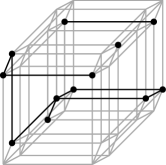
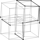
?figurename? 1: Depictions of the subgraph of the 5-dimensional hypercube graph induced by a typical random Boolean relation with 12 elements. Left: highlighted on an orthographic hypercube projection by our SatConn-tool. Center: highlighted on a “Spectral Embedding” of the hypercube graph by Mathematica. Right: the sole subgraph, arranged by Mathematica.

            

?figurename? 2: Subgraphs of the 8-dimensional hypercube graph (with 256 vertices) induced by typical random relations with 40, 60 and 80 elements, arranged by Mathematica.

Our perspective is mainly from complexity theory: As it was done for SAT and many of the related problems, we classify restrictions of the connectivity problems by their worst-case complexity. Along the way, we will also examine structural properties of the solution graph, and devise efficient algorithms for solving the connectivity problems.

Besides the usual propositional formulas with the connectives $\wedge$, $\vee$ and $\neg$, there are many alternative representations of Boolean relations; we will consider the following:

• Boolean constraint satisfaction problems (Boolean CSPs, here CSPs for short), specifically

  • CNF_C($\mathcal{S}$)-formulas, i.e. conjunctions of constraints that arise from inserting variables and constants in relations of some finite set $\mathcal{S}$,

  • CNF($\mathcal{S}$)-formulas, where no constants may be used,

• $B$-formulas, i.e. arbitrarily nested formulas built from some finite set $B$ of connectives,

• $B$-circuits, i.e. Boolean circuits where the gates are from some finite set $B$.

For CNF_C($\mathcal{S}$)-formulas and $B$-formulas, we also consider versions with quantifiers.

2 Relevance of Solution Space Connectivity

A direct application of $st$-connectivity in solution graphs are reconfiguration problems, that arise when we wish to find a step-by-step transformation between two feasible solutions of a problem, such that all intermediate results are also feasible. Recently, the reconfiguration versions of many problems such as Independent-Set, Vertex-Cover, Set-Cover Graph-$k$-Coloring, Shortest-Path have been studied (see e.g. [22, 23]).

The connectivity properties of solution graphs are also of relevance to the problem of structure identification, where one is given a relation explicitly and seeks a short representation of some kind (see e.g. [13]); this problem is important especially for learning in artificial intelligence.

Further, a better understanding of the solution space structure promises advancement of SAT algorithms: It has been discovered that the solution space connectivity is strongly correlated to the performance of standard satisfiability algorithms like WalkSAT and DPLL on random instances: As one approaches the satisfiability threshold (the ratio of constraints to variables at which random $k$-CNF-formulas become unsatisfiable for $k\geq 3$) from below, the solution space (with the connectivity defined as above) fractures, and the performance of the algorithms deteriorates [26, 25]. These insights mainly came from statistical physics, and lead to the development of the survey propagation algorithm, which has superior performance on random instances [25].

While current SAT solvers normally accept only CNF-formulas as input, in EDA the instances mostly derive from digital circuit descriptions [40], and although many such instances can easily be encoded in CNF, the original structural information, such as signal ordering, gate orientation and logic paths, is lost, or at least obscured. Since exactly this information can be very helpful for solving these instances, considerable effort has been made recently to develop satisfiability solvers that work with the circuit description directly [40], which have far better performance in EDA applications, or to restore the circuit structure from CNF [16]. This is a reason for us to study the solution space also for Boolean circuits.

3 Related Work, Prior Publications, and this Thesis

Research has focused on the solution space structure only quite recently: Complexity results for the connectivity problems in the solution graphs of CSPs have first been obtained in 2006 by P. Gopalan, P. G. Kolaitis, E. Maneva, and C. H. Papadimitriou [18, 19]. In particular, they investigated CNF_C($\mathcal{S}$)-formulas and studied

• the $st$-connectivity problem st-Conn_C($\mathcal{S}$), that asks for a CNF_C($\mathcal{S}$)-formula $\phi$ and two solutions $\boldsymbol{s}$ and $\boldsymbol{t}$ whether there a path from $\boldsymbol{s}$ to $\boldsymbol{t}$ in $G(\phi)$,

• the connectivity problem Conn_C($\mathcal{S}$), that asks for a CNF_C($\mathcal{S}$)-formula $\phi$ whether $G(\phi)$ is connected,

and

• the maximal diameter of any connected component of $G(\phi)$ for a CNF_C($\mathcal{S}$)-formula $\phi$, where the diameter of a component is the maximal shortest-path distance between any two vectors in that component.

They found a common structural and computational dichotomy: On one side, the maximal diameter is linear in the number of variables, $st$-connectivity is in P and connectivity is in coNP, while on the other side, the diameter can be exponential, and both problems are PSPACE-complete. Moreover, they conjectured a trichotomy for connectivity: That it is in P, coNP-complete, or PSPACE-complete. Together with Makino et al. [28], they already proved parts of this trichotomy.

In [34], we completed the proof of the trichotomy, and also corrected minor mistakes in [19], which lead to a slight shift of the boundaries towards the hard side. So for CNF_C($\mathcal{S}$)-formulas, we now have a quite complete picture, which we present in Chapter 1. In [34], we explained in detail the mistakes of Gopalan et al. and their implications, here we just give the correct statement and proofs.

In Chapter 2, we investigate two important variants: CNF($\mathcal{S}$)-formulas without constants, and partially quantified CNF_C($\mathcal{S}$)-formulas. In both cases, we prove a dichotomy for $st$-connectivity and the diameter analogous to the one for CNF_C($\mathcal{S}$)-formulas. For for the connectivity problem, we prove a trichotomy in the case of quantified formulas, while in the case of formulas without constants, we have no complete classification, but identify fragments where the problem is in P, where it is coNP-complete, and where it is PSPACE-complete. Of this chapter, only a preprint with preliminary results appeared on ArXiv [36].

Finally, in Chapter 3, we look at $B$-formulas and $B$-circuits. Here, we find a common dichotomy for the diameter and both connectivity problems: on one side, the diameter is linear and both problems are in P, while on the other, the diameter can be exponential, and the problems are PSPACE-complete. For quantified $B$-formulas, we prove an analogous dichotomy. The work in this chapter has been published in [35].

4 Associated Software

As part of the research for this thesis, several programs were written, some of which may be useful for future work on related problems. All software is written in Java (version 8) and provided in the SatConn package at https://github.com/konradws/SatConn, including a graphical tool to draw the solution graphs on hypercube projections, used for several graphics in this thesis.

After downloading the complete repository, the folder can be opened resp. imported in Netbeans or Eclipse as a project. The graphical tool is also provided as executable (SatConnTool.jar).

The most useful functions are declared public and equipped with Javadoc comments, where helpful. The main-functions provide usage examples and can be executed by running the respective file.

5 General Preliminaries

Prerequisites

We assume familiarity with some basic concepts from theoretical computer science, especially complexity theory, and its mathematical foundations:

• From mathematics, we require propositional logic, and basics about graphs, hypergraphs, and lattices,

• From theoretical computer science, we require Turing machines, the common complexity classes P, NP, coNP, PSPACE, and polynomial-time reductions.

Notation

We use $\boldsymbol{a},\boldsymbol{b},\ldots$ or $\boldsymbol{a}^{1},\boldsymbol{a}^{2},\ldots$ to denote vectors of Boolean values and $\boldsymbol{x},\boldsymbol{y},\ldots$ or $\boldsymbol{x}^{1},\boldsymbol{x}^{2},\ldots$ to denote vectors of variables, $\boldsymbol{a}=(a_{1},a_{2},\ldots)$ and $\boldsymbol{x}=(x_{1},x_{2},\ldots)$.

$\phi[\boldsymbol{x}^{i}/\boldsymbol{a}]$ denotes the formula resulting from $\phi$ by substituting the constants $a_{j}$ for the variables $x_{j}^{i}$.

The symbol $\leq_{m}^{p}$ is used for polynomial-time many-one reductions.

Central concepts

In the following definition, we formally introduce some concepts related to solution space connectivity in general. At the beginning of the next chapter, we define notions specific to CSPs. A reader only interested in $B$-formulas and $B$-circuits may read Section 3 after the next definition, and then skip to Chapter 3.

Definition 5.1.

An $n$-ary Boolean relation (or logical relation, relation for short) is a subset of $\{0,1\}^{n}$ for some integer $n\geq 1$.

The set of solutions of a propositional formula $\phi$ over $n$ variables defines in a natural way an $n$-ary relation $[\phi]$, where the variables are taken in lexicographic order. We will often identify the formula $\phi$ with the relation it defines and omit the brackets.

The solution graph $G(\phi)$ of $\phi$ then is the subgraph of the $n$-dimensional hypercube graph induced by the vectors in $[\phi]$. We will also refer to $G(R)$ for any logical relation $R$ (not necessarily defined by a formula).

The Hamming weight $|\boldsymbol{a}|$ of a Boolean vector $\boldsymbol{a}$ is the number of 1’s in $\boldsymbol{a}$. For two vectors $\boldsymbol{a}$ and $\boldsymbol{b}$, the Hamming distance $|\boldsymbol{a}-\boldsymbol{b}|$ is is the number of positions in which they differ.

If $\boldsymbol{a}$ and $\boldsymbol{b}$ are solutions of $\phi$ and lie in the same connected component (component for short) of $G(\phi)$, we write $d_{\phi}(\boldsymbol{a},\boldsymbol{b})$ to denote the shortest-path distance between $\boldsymbol{a}$ and $\boldsymbol{b}$. The diameter of a component is the maximal shortest-path distance between any two vectors in that component. The diameter of $G(\phi)$ is the maximal diameter of any of its connected components.

?chaptername? 1 Connectivity of Constraints

We start our investigation with constraint satisfaction problems. A constraint is a tuple of variables together with a Boolean relation, restricting the assignment of the variables. A CSP then is the question whether there is an assignment to all variables of a set of constraints such that all constraints are satisfied.

1 Preliminaries

1 CNF-Formulas and Schaefer’s Framework

In line with Gopalan et al., we define CSPs by CNF($\mathcal{S}$)-formulas, which were introduced in 1978 by Thomas Schaefer as a generalization of CNF (conjunctive normal form) formulas [32].

Definition 1.1.

A CNF-formula is a propositional formula of the form $C_{1}\wedge\cdots\wedge C_{m}$ ($1\leq m<\infty$), where each $C_{i}$ is a clause, that is, a finite disjunction of literals (variables or negated variables). A $k$-CNF-formula ($k\geq 1$) is a CNF-formula where each $C_{i}$ has at most $k$ literals. A Horn (dual Horn) formula is a CNF-formula where each $C_{i}$ has at most one positive (negative) literal.

Definition 1.2.

For a finite set of relations $\mathcal{S}$, a CNF_C($\mathcal{S}$)-formula over a set of variables $V$ is a finite conjunction $C_{1}\wedge\cdots\wedge C_{m}$, where each $C_{i}$ is a constraint application (constraint for short), i.e., an expression of the form $R(\xi_{1},\ldots,\xi_{k})$, with a $k$-ary relation $R\in\mathcal{S}$, and each $\xi_{j}$ is a variable from $V$ or one of the constants {0, 1}. A CNF($\mathcal{S}$)-formula is a CNF_C($\mathcal{S}$)-formula where each $\xi_{j}$ is a variable in $V$, not a constant.

By $\mathrm{Var}(C_{i})$, we denote the set of variables occurring in $\xi_{1},\ldots,\xi_{k}$. With the relation corresponding to $C_{i}$ we mean the relation $[R(\xi_{1},\ldots,\xi_{k})]$ (that may be different from $R$ by substitution of constants, and identification and permutation of variables).

A $k$-clause is a disjunction of $k$ variables or negated variables. For $0\leq i\leq k$, let $D_{i}$ be the corresponding to the $k$-clause whose first $i$ literals are negated, and let $S_{k}=\{D_{0},\ldots,D_{k}\}$, e.g., $\mathcal{S}_{3}=\{[x\vee y\vee z],\>[\overline{x}\vee y\vee z],\>[\overline{x}\vee\overline{y}\vee z],\>[\overline{x}\vee\overline{y}\vee\overline{z}]\}$. Thus, CNF($S_{k}$) is the collection of $k$-CNF-formulas.

Thomas Schaefer introduced CNF($\mathcal{S}$)-formulas for expressing variants of Boolean satisfiability; in his dichotomy theorem, Schaefer then classified the complexity of the satisfiability problem for CNF_C($\mathcal{S}$)- and CNF($\mathcal{S}$)-formulas [32]; we will do so here for the connectivity problems. We use the following notation:

• Sat($\mathcal{S}$) for the satisfiability problem: Given a CNF($\mathcal{S}$)-formula $\phi$, is $\phi$ satisfiable?

• st-Conn($\mathcal{S}$) for the $st$-connectivity problem: Given a CNF($\mathcal{S}$)-formula $\phi$ and two solutions $\boldsymbol{s}$ and $\boldsymbol{t}$, is there a path from $\boldsymbol{s}$ to $\boldsymbol{t}$ in $G(\phi)$?

• Conn($\mathcal{S}$) for the connectivity problem: Given a CNF($\mathcal{S}$)-formula $\phi$, is $G(\phi)$ connected? (if $\phi$ is unsatisfiable, we consider $G(\phi)$ connected)

The respective problems for CNF_C($\mathcal{S}$)-formulas are marked with the subscript _C. Note that Gopalan et al. considered the case with constants, but omitted the _C.

2 Classes of Relations

In the following definition, we introduce the types of relations needed for the classifications. Some are already familiar from Schaefer’s dichotomy theorem, some were introduced by Gopalan et al., and the ones starting with “safely” we defined in [34] to account for the shift of the boundaries resulting from Gopalan et al.’s mistake; IHSB stands for “implicative hitting set-bounded” and was introduced in [11].

Definition 1.3.

Let $R$ be an $n$-ary logical relation.

• $R$ is 0-valid (1-valid) if $0^{n}\in R$ ($1^{n}\in R$).

• $R$ is complementive if for every vector $(a_{1},\ldots,a_{n})\in R$, also $(a_{1}\oplus 1,\ldots,a_{n}\oplus 1)\in R$.

• $R$ is bijunctive if it is the set of solutions of a 2-CNF-formula.

• $R$ is Horn (dual Horn) if it is the set of solutions of a Horn (dual Horn) formula.

• $R$ is affine if it is the set of solutions of a formula $x_{i_{1}}\oplus\ldots\oplus x_{i_{m}}\oplus c$ with $i_{1},\ldots,i_{m}\in\{1,\ldots,n\}$ and $c\in\{0,1\}$.

• $R$ is componentwise bijunctive if every connected component of $G(R)$ is a bijunctive relation. $R$ is safely componentwise bijunctive if $R$ and every relation $R^{\prime}$ obtained from $R$ by identification of variables is componentwise bijunctive.

• $R$ is OR-free (NAND-free) if the relation OR = $\left\{01,10,11\right\}$ (NAND = $\left\{00,01,10\right\}$) cannot be obtained from $R$ by substitution of constants. $R$ is safely OR-free (safely NAND-free) if $R$ and every relation $R^{\prime}$ obtained from $R$ by identification of variables is OR-free (NAND-free).

• $R$ is IHSB$-$ (IHSB$+$) if it is the set of solutions of a Horn (dual Horn) formula in which all clauses with more than 2 literals have only negative literals (only positive literals).

• $R$ is componentwise IHSB$-$ (componentwise IHSB$+$) if every connected component of $G(R)$ is IHSB$-$ (IHSB$+$). $R$ is safely componentwise IHSB$-$ (safely componentwise IHSB$+$) if $R$ and every relation $R^{\prime}$ obtained from $R$ by identification of variables is componentwise IHSB$-$ (componentwise IHSB$+$).

If one is given the relation explicitly (as a set of vectors), the properties 0-valid, 1-valid, complementive, OR-free and NAND-free can be checked straightforward, while bijunctive, Horn, dual Horn, affine, IHSB$-$ and IHSB$+$ can be checked by closure properties:

Definition 1.4.

A relation $R$ is closed under some $n$-ary operation $f$ iff the vector obtained by the coordinate-wise application of $f$ to any $m$ vectors from $R$ is again in $R$, i.e., if

$$\boldsymbol{a}^{1},\ldots,\boldsymbol{a}^{m}\in R\Longrightarrow\left(f(a_{1}^{1},\ldots,a_{1}^{m}),\ldots,f(a_{n}^{1},\ldots,a_{n}^{m})\right)\in R.$$

Lemma 1.5.

A relation $R$ is

1. bijunctive, iff it is closed under the ternary majority operation
   maj($x,y,z$)=$\left(x\vee y\right)\wedge\left(y\vee z\right)\wedge\left(z\vee x\right)$,

2. Horn (dual Horn), iff it is closed under $\wedge$ (under $\vee$, resp.),

3. affine, iff it is closed under $x\oplus y\oplus z$,

4. IHSB$-$ (IHSB$+$), iff it is closed under $x\wedge(y\vee z)$ (under $x\vee(y\wedge z)$, resp.).

?proofname? .

1. See [11, Lemma 4.9].

2. See [11, Lemma 4.8].

3. See [11, Lemma 4.10].

4. This can be verified using the Galois correspondence between closed sets of relations and closed sets of Boolean functions (see [8]): From the table (Fig. 1) in [8], we find that the IHSB$-$ relations are a base of the co-clone INV($\mathsf{S}_{10}$), and the IHSB$+$ ones a base of INV($\mathsf{S}_{00}$), and from the table (Figure 1) in [7], we see that $x\wedge(y\vee z)$ and $x\vee(y\wedge z)$ are bases of the clones $\mathsf{S}_{10}$ and $\mathsf{S}_{00}$, resp.∎

Remark 1.6.

The class Check of SatConn provides functions to check the properties of Definition 1.3, and the class Clones provides functions to calculate the clone and co-clone of a relation.

The closure properties carry over from a relation to its connected components, as shown by Gopalan et al.:

Lemma 1.7.

[19, Lemma 4.1]  If a logical relation $R$ is closed under an operation $\alpha:\{0,1\}^{k}\rightarrow\{0,1\}$ such that $\alpha(1,\ldots,1)=1$ and $\alpha(0,\ldots,0)=0$ (a.k.a. an idempotent operation), then every connected component of $G(R)$ is closed under $\alpha$.

3 Classes of Sets of Relations

The classes in the following definition demarcate the structural and computational boundaries for the solution graphs of CNF_C($\mathcal{S}$)-formulas.

Definition 1.8.

A set $\mathcal{S}$ of logical relations is safely tight if at least one of the following conditions holds:

1. Every relation in $\mathcal{S}$ is safely componentwise bijunctive.

2. Every relation in $\mathcal{S}$ is safely OR-free .

3. Every relation in $\mathcal{S}$ is safely NAND-free.

A set $\mathcal{S}$ of logical relations is Schaefer if at least one of the following conditions holds:

1. Every relation in $\mathcal{S}$ is bijunctive.

2. Every relation in $\mathcal{S}$ is Horn.

3. Every relation in $\mathcal{S}$ is dual Horn.

4. Every relation in $\mathcal{S}$ is affine.

A set $\mathcal{S}$ of logical relations is CPSS if at least one of the following conditions holds:

1. Every relation in $\mathcal{S}$ is bijunctive.

2. Every relation in $\mathcal{S}$ is Horn and safely componentwise IHSB$-$.

3. Every relation in $\mathcal{S}$ is dual Horn and safely componentwise IHSB$+$.

4. Every relation in $\mathcal{S}$ is affine.

A single logical relation $R$ is safely tight, Schaefer, or CPSS, if $\{R\}$ has that property. Vice versa, we say that a set $\mathcal{S}$ of logical relations has one of the properties from Definition 1.3 if every relation in $\mathcal{S}$ has that property, e.g., $\mathcal{S}$ is 0-valid if every relation in $\mathcal{S}$ is 0-valid.

The term tight was introduced by Gopalan et al. because of the structural properties of the formulas built from tight (actually, only safely tight) relations, see Lemma 5.1 and Lemma 5.4. We introduced the CPSS class in [34]; CPSS stands for “constraint-projection separating Schaefer”, which will become clear in Section 6 from Definition 6.1, Lemma 6.4 and Lemma 8.1.

From the definition we see that every CPSS set of relations is also Schaefer, and we can show that it also holds that every Schaefer set is safely tight, by modifying a lemma of Gopalan et al.:

Lemma 1.9.

[modified from 19, Lemma 4.2]  Let $R$ be a logical relation.

1. If $R$ is bijunctive, then it is safely componentwise bijunctive.

2. If $R$ is Horn, then it is safely OR-free.

3. If $R$ is dual Horn, then it is safely NAND-free.

4. If $R$ is affine, then it is safely componentwise bijunctive, safely OR-free, and safely NAND-free.

?proofname?.

We first note that

• any relation obtained from a bijunctive (Horn, dual Horn, affine) one by identification of variables is itself bijunctive (Horn, dual Horn, affine),

which is obvious from the definitions.

If $R$ is bijunctive, it is closed under maj, which is idempotent, so by Lemma 1.7, $R$ is also componentwise bijunctive, and by (*), it is safely componentwise bijunctive as well.

The cases of Horn and dual Horn are symmetric. Suppose a $r$-ary Horn relation $R$ is not OR-free. Then there exist $i,j\in\{1,\dots,r\}$ and constants $t_{1},\dots,t_{r}\in\{0,1\}$ such that the relation $R(t_{1},\dots,t_{i-1},x,t_{i+1},\dots,t_{j-1},y,t_{j+1},\dots,t_{r})$ on variables $x$ and $y$ is equivalent to $x\vee y$, i.e.

$$R(t_{1},\dots,t_{i-1},x,t_{i+1},\dots,t_{j-1},y,t_{j+1},\dots,t_{r})=\{01,11,10\}.$$

Thus the tuples $\boldsymbol{t^{00}},\boldsymbol{t^{01}}\boldsymbol{t^{10}},\boldsymbol{t^{11}}$ defined by $(t_{i}^{ab},t_{j}^{ab})=(a,b)$ and $t_{k}^{ab}=t_{k}$ for every $k\not\in\{i,j\}$, where $a,b,\in\{0,1\}$ satisfy $\boldsymbol{t^{10}},\boldsymbol{t^{11}},\boldsymbol{t^{01}}\in R$ and $\boldsymbol{t^{00}}\not\in R$. However, since every Horn relation is closed under $\wedge$, it follows that $\boldsymbol{t^{01}}\wedge\boldsymbol{t^{10}}=\boldsymbol{t^{00}}$ must be in $R$, which is a contradiction. So $R$ is OR-free, and again by (*), it must be safely OR-free as well.

For the affine case, a small modification of the last step of the above argument shows that an affine relation also is OR-free; therefore, dually, it is also NAND-free. Namely, since a relation $R$ is affine if and only if it is closed under ternary $\oplus$, it follows that $\boldsymbol{t^{01}}\oplus\boldsymbol{t^{11}}\oplus\boldsymbol{t^{10}}=\boldsymbol{t^{00}}$ must be in $R$. Since the connected components of an affine relation are both OR-free and NAND-free the subgraphs that they induce are hypercubes, which are also bijunctive relations. Therefore an affine relation is also componentwise bijunctive. With this, it must also be safely OR-free, safely OR-free and safely componentwise bijunctive by (*). ∎

2 Results

We are now ready to state the results for CNF_C($\mathcal{S}$)-formulas; in the subsequent sections we will prove them. The following two theorems give complete classifications up to polynomial-time isomorphisms. They are summarized in the table below.

$\mathcal{S}$	SatC($\mathcal{S}$)	ConnC($\mathcal{S}$)	st-ConnC($\mathcal{S}$)	Diameter
not safely tight	NP-complete	PSPACE-complete	PSPACE-complete	$2^{\Omega(\sqrt{n})}$
safely tight, not Schaefer		coNP-complete	in P	$O(n)$
Schaefer, not CPSS	in P
CPSS		in P

?tablename? 1: Our classifications for CNF_C($\mathcal{S}$)-formulas, in comparison to Sat.

Theorem 2.1 (Dichotomy theorem for st-Conn_C($\mathcal{S}$) and the diameter).

Let $\mathcal{S}$ be a finite set of logical relations.

1. If $\mathcal{S}$ is safely tight, st-Conn_C($\mathcal{S}$) is in P, and for every CNF_C($\mathcal{S}$)-formula $\phi$, the diameter of $G(\phi)$ is linear in the number of variables.

2. Otherwise, st-Conn_C($\mathcal{S}$) is PSPACE-complete, and there are CNF_C($\mathcal{S}$)-formulas $\phi$, such that the diameter of $G(\phi)$ is exponential in the number of variables.

?proofname?.

1. See Lemma 5.6.

2. See Corollary 4.9.∎

Theorem 2.2 (Trichotomy theorem for Conn_C($\mathcal{S}$)).

Let $\mathcal{S}$ be a finite set of logical relations.

1. If $\mathcal{S}$ is CPSS, Conn_C($\mathcal{S}$) is in P.

2. Else if $\mathcal{S}$ is safely tight, Conn_C($\mathcal{S}$) is coNP-complete.

3. Else, Conn_C($\mathcal{S}$) is PSPACE-complete.

?proofname?.

1. See Corollary 6.6.

2. See Corollary 7.11.

3. See Corollary 4.9. ∎

3 The General Case: Reduction from a Turing Machine

We start with the general case. Gopalan et al. showed that for 3-CNF-formulas, st-Conn_C and Conn_C are PSPACE-complete, and the diameter can be exponential:

Lemma 3.1.

[19, Lemma 3.6]  For general CNF-formulas, as well as for 3-CNF-formulas, st-Conn_C and Conn_C are $\mathrm{PSPACE}$-complete.

Showing that the problems are in PSPACE is straightforward: Given a CNF-formula $\phi$ and two solutions $\boldsymbol{s}$ and $\boldsymbol{t}$, we can guess a path of length at most $2^{n}$ between them and verify that each vertex along the path is indeed a solution. Hence st-Conn is in $\mathrm{NPSPACE}$, which equals PSPACE by Savitch’s theorem. For Conn, by reusing space we can check for all pairs of vectors whether they are satisfying, and, if they both are, whether they are connected in $G(\phi)$.

The hardness-proof is quite intricate: it consists of a direct reduction from the computation of a space-bounded Turing machine $M$. The input-string $w$ of $M$ is mapped to a 3-CNF-formula $\phi$ and two satisfying assignments $\boldsymbol{s}$ and $\boldsymbol{t}$, corresponding to the initial and accepting configuration of a Turing machine $M^{\prime}$ constructed from $M$ and $w$, s.t. $\boldsymbol{s}$ and $\boldsymbol{t}$ are connected in $G(\phi)$ iff $M$ accepts $w$. Further, all satisfying assignments of $\phi$ are connected to either $\boldsymbol{s}$ or $\boldsymbol{t}$, so that $G(\phi)$ is connected iff $M$ accepts.

Lemma 3.2.

[19, Lemma 3.7]  For $n$ even, there is a 3-CNF-formula $\phi_{n}$ with $n$ variables and $O(n^{2})$ clauses, s.t. $G(\phi_{n})$ is a path of length greater than $2^{\frac{n}{2}}$.

The proof of this lemma is by direct construction of such a formula.

4 Extension of PSPACE-Completeness: Structural Expressibility

To show that PSPACE-hardness and exponential diameter extend to all not (safely) tight sets of relations, Gopalan et al. used the concept of structural expressibility, which is a modification of Schaefer’s “representability” that he used for his dichotomy theorem, so let us have a quick look at this first:

Theorem 4.1 (Schaefer’s dichotomy theorem [32]).

Let $\mathcal{S}$ be a finite set of logical relations.

1. If $\mathcal{S}$ is Schaefer, then Sat_C($\mathcal{S}$) is in P; otherwise, Sat_C($\mathcal{S}$) is NP-complete.

2. If $\mathcal{S}$ is 0-valid, 1-valid, or Schaefer, then Sat($\mathcal{S}$) is in P; otherwise, Sat($\mathcal{S}$) is NP-complete.

Schaefer first proved statement 1, and from that derived the no-constants version; we here discuss only the proof statement 1.

Schaefer used a reduction from satisfiability of 3-CNF-formulas, i.e. CNF_C($\mathcal{S}_{3}$)-formulas (see Definition 1.2), which was already known to be NP-complete by the Cook–Levin theorem. Therefor, he exploited that any existentially quantified formula is satisfiability-equivalent to the formula with the quantifiers removed, and introduced the notion of representability, that became also know as expressibility:

Definition 4.2.

A relation $R$ is expressible from a set of relations $\mathcal{S}$ if there is a CNF_C($\mathcal{S}$)-formula $\phi(\boldsymbol{x},\boldsymbol{y})$ such that $R=\{\boldsymbol{a}|\exists\boldsymbol{y}\phi(\boldsymbol{a},\boldsymbol{y})\}$.

He then showed that every Boolean relation is expressible from any set of relations that is not Schaefer, and that this expression can efficiently be constructed.

With this, it is easy to see that for every non-Schaefer set $\mathcal{S}$, satisfiability of any CNF_C($\mathcal{S}_{3}$)-formula $\psi$ can be reduced to satisfiability of a CNF_C($\mathcal{S}$)-formula, constructed as follows: Replace in $\psi$ every constraint $R(\boldsymbol{\xi})$ by $\phi(\boldsymbol{\xi},\boldsymbol{y})$ with $\phi$ from Definition 4.2, and new variables $\boldsymbol{y}$, distinct for each constraint.

As Gopalan et al. explain in section 3.1 of [19], for the connectivity problems, expressibility is not sufficient; therefore, they introduced structural expressibility:

Definition 4.3.

A relation $R$ is structurally expressible from a set of relations $\mathcal{S}$ if there is a CNF_C($\mathcal{S}$)-formula $\phi$ such that the following conditions hold:

1. $R=\{\boldsymbol{a}|\exists\boldsymbol{y}\phi(\boldsymbol{a},\boldsymbol{y})\}$.

2. For every $\boldsymbol{a}\in R$, the graph $G(\phi(\boldsymbol{a},\boldsymbol{y}))$ is connected.

3. For $\boldsymbol{a},\boldsymbol{b}\in R$ with $|\boldsymbol{a}-\boldsymbol{b}|=1$, there exists a witness $\boldsymbol{w}$ such that $(\boldsymbol{a},\boldsymbol{w})$ and $(\boldsymbol{b},\boldsymbol{w})$ are solutions of $\phi$.

Gopalan et al. now argued that connectivity were retained when replacing every constraint $R$ with a structural expression of $R$ in a CNF_C($\mathcal{S}$)-formula. In fact, this is only true for CNF_C($\mathcal{S}$)-formulas where no variable is used more than once in any constraint, and their proof is only correct for such formulas that also use no constants:

Lemma 4.4.

[corrected from 19, Lemma 3.2]  Let $\mathcal{S}$ and $\mathcal{S}^{\prime}$ be sets of relations such that every $R\in\mathcal{S}^{\prime}$ is structurally expressible from $\mathcal{S}$. Given a CNF($\mathcal{S}^{\prime}$)-formula $\psi(\boldsymbol{x})$ (without constants), where no variable is used more than once in any constraint, one can efficiently construct a CNF_C($\mathcal{S}$)-formula $\varphi(\boldsymbol{x},\boldsymbol{y})$ such that

1. $\psi(\boldsymbol{x})=\exists\boldsymbol{y}\varphi(\boldsymbol{x},\boldsymbol{y})$;

2. if $(\boldsymbol{s}\boldsymbol{,w^{s}}),$ $(\boldsymbol{t},\boldsymbol{w^{t}})$ are connected in $G(\varphi)$ by a path of length $d$, then there is a path from $\boldsymbol{s}$ to $\boldsymbol{t}$ in $G(\psi)$ of length at most $d$;

3. if $\boldsymbol{s},\boldsymbol{t}\in\psi$ are connected in $G(\psi)$, then for every witness $\boldsymbol{w^{s}}$ of $\boldsymbol{s}$, and every witness $\boldsymbol{w^{t}}$ of $\boldsymbol{t}$, there is a path from $(\boldsymbol{s}\boldsymbol{,w^{s}})$ to $(\boldsymbol{t},\boldsymbol{w^{t}})$ in $G(\varphi)$.

In Gopalan et al.’s proof, we only clarify the notation a little:

?proofname?.

Let $\psi(\boldsymbol{x})=C_{1}\wedge\cdots\wedge C_{m}$ with $C_{j}=R_{j}(\boldsymbol{x}_{j})$, where $R_{j}$ is some relation from $\mathcal{S}^{\prime}$, and $\boldsymbol{x}_{j}$ is the vector of variables to which $R_{j}$ is applied. Let $\varphi_{j}$ be the structural expression for $R_{j}$ from ${\cal S}$, so that $R_{j}(\boldsymbol{x}_{j})\equiv\exists\boldsymbol{y}_{j}\leavevmode\nobreak\ \varphi_{j}(\boldsymbol{x}_{j},\boldsymbol{y}_{j})$. Let $\boldsymbol{y}$ be the vector $(\boldsymbol{y}_{1},\dots,\boldsymbol{y}_{m})$ and let $\varphi(\boldsymbol{x},\boldsymbol{y})$ be the formula $\wedge_{j=1}^{m}\varphi_{j}(\boldsymbol{x}_{j},\boldsymbol{y}_{j})$. Then $\psi(\boldsymbol{x})\equiv\exists\boldsymbol{y}\leavevmode\nobreak\ \varphi(\boldsymbol{x},\boldsymbol{y})$.

Statement $2$ follows from 1 by projection of the path on the coordinates of $\boldsymbol{x}$. For statement 3, consider $\boldsymbol{s},\boldsymbol{t}\in\psi$ that are connected in $G(\psi)$ via a path $\boldsymbol{s}=\boldsymbol{u^{0}}\rightarrow\boldsymbol{u^{1}}\rightarrow\dots\rightarrow\boldsymbol{u^{r}}=\boldsymbol{t}$ . For every $\boldsymbol{u^{i}},\boldsymbol{u^{i+1}}$, and clause $C_{j}$, there exists an assignment $\boldsymbol{w_{j}^{i}}$ to $\boldsymbol{y}_{j}$ such that both $(\boldsymbol{u_{j}^{i}},\boldsymbol{w_{j}^{i}})$ and $(\boldsymbol{u_{j}^{i+1}},\boldsymbol{w_{j}^{i}})$ are solutions of $\varphi_{j}$, by condition 3 of structural expressibility. Thus $(\boldsymbol{u^{i}},\boldsymbol{w^{i}})$ and $(\boldsymbol{u^{i+1}},\boldsymbol{w^{i}})$ are both solutions of $\varphi$, where $\boldsymbol{w^{i}}=(\boldsymbol{w_{1}^{i}},\dots,\boldsymbol{w_{m}^{i}})$. Further, for every $\boldsymbol{u^{i}}$, the space of solutions of $\varphi(\boldsymbol{u^{i}},\boldsymbol{y})$ is the product space of the solutions of $\varphi_{j}(\boldsymbol{u_{j}^{i}},\boldsymbol{y}_{j})$ over $j=1,\dots,m$. Since these are all connected by condition 2 of structural expressibility, $G(\varphi(\boldsymbol{u^{i}},\boldsymbol{y}))$ is connected. The following describes a path from $(\boldsymbol{s},\boldsymbol{w^{s}})$ to $(\boldsymbol{t},\boldsymbol{w^{t}})$ in $G(\varphi)$:  $(\boldsymbol{s},\boldsymbol{w^{s}})\rightsquigarrow(\boldsymbol{s},\boldsymbol{w^{0}})\rightarrow(\boldsymbol{u^{1}},\boldsymbol{w^{0}})\rightsquigarrow(\boldsymbol{u^{1}},\boldsymbol{w^{1}})\rightarrow\dots\rightsquigarrow(\boldsymbol{u^{r-1}},\boldsymbol{w^{r-1}})\rightarrow(\boldsymbol{t},\boldsymbol{w^{r-1}})\rightsquigarrow(\boldsymbol{t},\boldsymbol{w^{t}})$. Here $\rightsquigarrow$ indicates a path in $G(\varphi(\boldsymbol{u^{i}},\boldsymbol{y}))$. ∎

It is easy to show that the statement of Lemma 4.4 is also correct if we allow constants in $\psi$; however, we don’t need this result. In [34], we explain in detail the problem with repeated variables in constraint applications.

We have to change Gopalan et al.’s corollary accordingly; we denote the connectivity problems for CNF($\mathcal{S}$)-formulas without repeated variables in constraints (and without constants) by the subscript _ni:

Corollary 4.5.

[corrected from 19, Corollary 3.3]  Suppose $\mathcal{S}$ and $\mathcal{S}^{\prime}$ are sets of relations such that every $R\in\mathcal{S}^{\prime}$ is structurally expressible from $\mathcal{S}$.

1. There are polynomial-time reductions from Conn_ni($\mathcal{S}$’) to Conn_C($\mathcal{S}$), and from st-Conn_ni($\mathcal{S}$’) to st-Conn_C($\mathcal{S}$).

2. If there exists a CNF_ni($\mathcal{S}$’)-formula $\psi(\boldsymbol{x})$ with $n$ variables, $m$ clauses and diameter $d$, then there exists a CNF_C($\mathcal{S}$)-formula $\phi(\boldsymbol{x},\boldsymbol{y})$, where $\boldsymbol{y}$ is a vector of $O(m)$ variables, such that the diameter of $G(\phi)$ is at least $d$.

Since 3-CNF-fomulas are CNF_ni($\mathcal{S}_{1}\cup\mathcal{S}_{2}\cup\mathcal{S}_{3}$)-formulas, for the reductions to work it now remains to prove that $\mathcal{S}_{1}\cup\mathcal{S}_{2}\cup\mathcal{S}_{3}$ is structurally expressible from any not safely tight set. As Theorem 4.8 below shows, in fact every Boolean relation is structurally expressible from any such set. The long proof of the next lemma contains only minor modifications from [19].

Lemma 4.6.

[modified from 19, Lemma 3.4]  If a set $\mathcal{S}$ of relations is not safely tight, $\mathcal{S}_{3}$ is structurally expressible from $\mathcal{S}$.

?proofname?.

First, observe that all $2$-clauses are structurally expressible from ${\cal S}$. There exists $R\in{\cal S}$ which is not safely OR-free, so we can express $(x_{1}\vee x_{2})$ by substituting constants and identifying variables in $R$. Similarly, we can express $(\bar{x}_{1}\vee\bar{x}_{2})$ using a relation that is not safely NAND-free. The last 2-clause $(x_{1}\vee\bar{x}_{2})$ can be obtained from OR and NAND by a technique that corresponds to reverse resolution. $(x_{1}\vee\bar{x}_{2})=\exists y\leavevmode\nobreak\ (x_{1}\vee y)\wedge(\bar{y}\vee\bar{x}_{2})$. It is easy to see that this gives a structural expression. From here onwards we assume that ${\cal S}$ contains all 2-clauses. The proof now proceeds in four steps. First, we will express a relation in which there exist two elements that are at graph distance larger than their Hamming distance. Second, we will express a relation that is just a single path between such elements. Third, we will express a relation which is a path of length 4 between elements at Hamming distance 2. Finally, we will express the 3-clauses.

Step 1. Structurally expressing a relation in which some distance expands.
For a relation $R$, we say that the distance between $\boldsymbol{a}$ and $\boldsymbol{b}$ expands if $\boldsymbol{a}$ and $\boldsymbol{b}$ are connected in $G(R)$, but $d_{R}(\boldsymbol{a},\boldsymbol{b})>|\boldsymbol{a}-\boldsymbol{b}|$. Later on, we will show that no distance expands in safely componentwise bijunctive relations. The same also holds true for the relation $R_{{\rm{NAE}}}=\{0,1\}^{3}\setminus\{000,111\}$, which is not safely componentwise bijunctive. Nonetheless, we show here that if $R$ is not safely componentwise bijunctive, then, by adding $2$-clauses, we can structurally express a relation $Q$ in which some distance expands. For instance, when $R=R_{{\rm NAE}}$, then we can take $Q(x_{1},x_{2},x_{3})=R_{{\rm NAE}}(x_{1},x_{2},x_{3})\wedge(\bar{x_{1}}\vee\bar{x}_{3})$. The distance between $\boldsymbol{a}=100$ and $\boldsymbol{b}=001$ in $Q$ expands. Similarly, in the general construction, we identify $\boldsymbol{a}$ and $\boldsymbol{b}$ on a cycle, and add $2$-clauses that eliminate all the vertices along the shorter arc between $\boldsymbol{a}$ and $\boldsymbol{b}$.

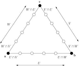
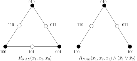
?figurename? 1: Proof of Step 1, and an example.

Since ${\cal S}$ is not safely tight, it contains a relation which is not safely componentwise bijunctive, from which we can obtain a not componentwise bijunctive relation $R$. If $R$ contains $\boldsymbol{a},\boldsymbol{b}$ where the distance between them expands, we are done. So assume that for all $\boldsymbol{a},\boldsymbol{b}\in G(R)$, $d_{R}(\boldsymbol{a},\boldsymbol{b})=|\boldsymbol{a}-\boldsymbol{b}|$. Since $R$ is not componentwise bijunctive, there exists a triple of assignments $\boldsymbol{a},\boldsymbol{b},\boldsymbol{c}$ lying in the same component such that $\mathrm{Maj}(\boldsymbol{a},\boldsymbol{b},\boldsymbol{c})$ is not in that component (which also easily implies it is not in $R$). Choose the triple such that the sum of pairwise distances $d_{R}(\boldsymbol{a},\boldsymbol{b})+d_{R}(\boldsymbol{b},\boldsymbol{c})+d_{R}(\boldsymbol{c},\boldsymbol{a})$ is minimized. Let $U=\{i|a_{i}\neq b_{i}\}$, $V=\{i|b_{i}\neq c_{i}\}$, and $W=\{i|c_{i}\neq a_{i}\}$. Since $d_{R}(\boldsymbol{a},\boldsymbol{b})=|\boldsymbol{a}-\boldsymbol{b}|$, a shortest path does not flip variables outside of $U$, and each variable in $U$ is flipped exactly once. The same holds for $V$ and $W$. We note some useful properties of the sets $U,V,W$.

1. Every index $i\in U\cup V\cup W$ occurs in exactly two of $U,V,W$.
   Consider going by a shortest path from $\boldsymbol{a}$ to $\boldsymbol{b}$ to $\boldsymbol{c}$ and back to $\boldsymbol{a}$. Every $i\in U\cup V\cup W$ is seen an even number of times along this path since we return to $\boldsymbol{a}$. It is seen at least once, and at most thrice, so in fact it occurs twice.

2. Every pairwise intersection $U\cap V,V\cap W$ and $W\cap U$ is non-empty.
   Suppose the sets $U$ and $V$ are disjoint. From Property 1, we must have $W=U\cup V$. But then it is easy to see that $\mathrm{Maj}(\boldsymbol{a},\boldsymbol{b},\boldsymbol{c})=\boldsymbol{b}$ which is in $R$. This contradicts the choice of $\boldsymbol{a},\boldsymbol{b},\boldsymbol{c}$.

3. The sets $U\cap V$ and $U\cap W$ partition the set $U$.
   By Property $1$, each index of $U$ occurs in one of $V$ and $W$ as well. Also since no index occurs in all three sets $U,V,W$ this is in fact a disjoint partition.

4. For each index $i\in U\cap W$, it holds that $\boldsymbol{a}\oplus\boldsymbol{e}_{i}\not\in R$.
   Assume for the sake of contradiction that $\boldsymbol{a^{\prime}}=\boldsymbol{a}\oplus\boldsymbol{e}_{i}\in R$. Since $i\in U\cap W$ we have simultaneously moved closer to both $\boldsymbol{b}$ and $\boldsymbol{c}$. Hence we have $d_{R}(\boldsymbol{a^{\prime}},\boldsymbol{b})+d_{R}(\boldsymbol{b},\boldsymbol{c})+d_{R}(\boldsymbol{c},\boldsymbol{a^{\prime}})<d_{R}(\boldsymbol{a},\boldsymbol{b})+d_{R}(\boldsymbol{b},\boldsymbol{c})+d_{R}(\boldsymbol{c},\boldsymbol{a})$. Also $\mathrm{Maj}(\boldsymbol{a^{\prime}},\boldsymbol{b},\boldsymbol{c})=\mathrm{Maj}(\boldsymbol{a},\boldsymbol{b},\boldsymbol{c})\not\in R$. But this contradicts our choice of $\boldsymbol{a},\boldsymbol{b},\boldsymbol{c}$.

Property 4 implies that the shortest paths to $\boldsymbol{b}$ and $\boldsymbol{c}$ diverge at $\boldsymbol{a}$, since for any shortest path to $\boldsymbol{b}$ the first variable flipped is from $U\cap V$ whereas for a shortest path to $\boldsymbol{c}$ it is from $W\cap V$. Similar statements hold for the vertices $\boldsymbol{b}$ and $\boldsymbol{c}$. Thus along the shortest path from $\boldsymbol{a}$ to $\boldsymbol{b}$ the first bit flipped is from $U\cap V$ and the last bit flipped is from $U\cap W$. On the other hand, if we go from $\boldsymbol{a}$ to $\boldsymbol{c}$ and then to $\boldsymbol{b}$, all the bits from $U\cap W$ are flipped before the bits from $U\cap V$. We use this crucially to define $Q$. We will add a set of 2-clauses that enforce the following rule on paths starting at $\boldsymbol{a}$: Flip variables from $U\cap W$ before variables from $U\cap V$. This will eliminate all shortest paths from $\boldsymbol{a}$ to $\boldsymbol{b}$ since they begin by flipping a variable in $U\cap V$ and end with $U\cap W$. The paths from $\boldsymbol{a}$ to $\boldsymbol{b}$ via $\boldsymbol{c}$ survive since they flip $U\cap W$ while going from $\boldsymbol{a}$ to $\boldsymbol{c}$ and $U\cap V$ while going from $\boldsymbol{c}$ to $\boldsymbol{b}$. However all remaining paths have length at least $|\boldsymbol{a}-\boldsymbol{b}|+2$ since they flip twice some variables not in $U$.

Take all pairs of indices $\{(i,j)|i\in U\cap W,j\in U\cap V\}$. The following conditions hold from the definition of $U,V,W$: $a_{i}=\bar{c}_{i}=\bar{b}_{i}$ and $a_{j}=c_{j}=\bar{b}_{j}$. Add the 2-clause $C_{ij}$ asserting that the pair of variables $x_{i}x_{j}$ must take values in $\{a_{i}a_{j},c_{i}c_{j},b_{i}b_{j}\}=\{a_{i}a_{j},\bar{a}_{i}a_{j},\bar{a}_{i}\bar{a}_{j}\}$. The new relation is $Q=R\wedge_{i,j}C_{ij}$. Note that $Q\subset R$. We verify that the distance between $\boldsymbol{a}$ and $\boldsymbol{b}$ in $Q$ expands. It is easy to see that for any $j\in U$, the assignment $\boldsymbol{a}\oplus\boldsymbol{e}_{j}\not\in Q$. Hence there are no shortest paths left from $\boldsymbol{a}$ to $\boldsymbol{b}$. On the other hand, it is easy to see that $\boldsymbol{a}$ and $\boldsymbol{b}$ are still connected, since the vertex $\boldsymbol{c}$ is still reachable from both.

Step 2. Isolating a pair of assignments whose distance expands.
The relation $Q$ obtained in Step 1 may have several disconnected components. This cleanup step isolates a single pair of assignments whose distance expands. By adding $2$-clauses, we show that one can express a path of length $r+2$ between assignments at distance $r$.

Take $\boldsymbol{a},\boldsymbol{b}\in Q$ whose distance expands in $Q$ and $d_{Q}(\boldsymbol{a},\boldsymbol{b})$ is minimized. Let $U=\{i|a_{i}\neq b_{i}\}$, and $|U|=r$. Shortest paths between $\boldsymbol{a}$ and $\boldsymbol{b}$ have certain useful properties:

1. Each shortest path flips every variable from $U$ exactly once.
   Observe that each index $j\in U$ is flipped an odd number of times along any path from $\boldsymbol{a}$ to $\boldsymbol{b}$. Suppose it is flipped thrice along a shortest path. Starting at $\boldsymbol{a}$ and going along this path, let $\boldsymbol{b^{\prime}}$ be the assignment reached after flipping $j$ twice. Then the distance between $\boldsymbol{a}$ and $\boldsymbol{b^{\prime}}$ expands, since $j$ is flipped twice along a shortest path between them in $Q$. Also $d_{Q}(\boldsymbol{a},\boldsymbol{b^{\prime}})<d_{Q}(\boldsymbol{a},\boldsymbol{b})$, contradicting the choice of $\boldsymbol{a}$ and $\boldsymbol{b}$.

2. Every shortest path flips exactly one variable $i\not\in U$.
   Since the distance between $\boldsymbol{a}$ and $\boldsymbol{b}$ expands, every shortest path must flip some variable $i\not\in U$. Suppose it flips more than one such variable. Since $\boldsymbol{a}$ and $\boldsymbol{b}$ agree on these variables, each of them is flipped an even number of times. Let $i$ be the first variable to be flipped twice. Let $\boldsymbol{b^{\prime}}$ be the assignment reached after flipping $i$ the second time. It is easy to verify that the distance between $\boldsymbol{a}$ and $\boldsymbol{b^{\prime}}$ also expands, but $d_{Q}(\boldsymbol{a},\boldsymbol{b^{\prime}})<d_{Q}(\boldsymbol{a},\boldsymbol{b})$.

3. The variable $i\not\in U$ is the first and last variable to be flipped along the path.
   Assume the first variable flipped is not $i$. Let $\boldsymbol{a^{\prime}}$ be the assignment reached along the path before we flip $i$ the first time. Then $d_{Q}(\boldsymbol{a^{\prime}},\boldsymbol{b})<d_{Q}(\boldsymbol{a},\boldsymbol{b})$. The distance between $\boldsymbol{a^{\prime}}$ and $\boldsymbol{b}$ expands since the shortest path between them flips the variables $i$ twice. This contradicts the choice of $\boldsymbol{a}$ and $\boldsymbol{b}$. Assume $j\in U$ is flipped twice. Then as before we get a pair $\boldsymbol{a^{\prime}},\boldsymbol{b^{\prime}}$ that contradict the choice of $\boldsymbol{a},\boldsymbol{b}$.

Every shortest path between $\boldsymbol{a}$ and $\boldsymbol{b}$ has the following structure: first a variable $i\not\in U$ is flipped to $\bar{a}_{i}$, then the variables from $U$ are flipped in some order, finally the variable $i$ is flipped back to $a_{i}$.

Different shortest paths may vary in the choice of $i\not\in U$ in the first step and in the order in which the variables from $U$ are flipped. Fix one such path $T\subseteq Q$. Assume that $U=\{1,\dots,r\}$ and the variables are flipped in this order, and the additional variable flipped twice is $r+1$. Denote the path by $\boldsymbol{a}\rightarrow\boldsymbol{u^{0}}\rightarrow\boldsymbol{u^{1}}\rightarrow\dots\rightarrow\boldsymbol{u^{r}}\rightarrow\boldsymbol{b}$. Next we prove that we cannot flip the $r+1^{th}$ variable at an intermediate vertex along the path.

1. For $1\leq j\leq r-1$ the assignment $\boldsymbol{u^{j}}\oplus\boldsymbol{e_{r+1}}\not\in Q$. Suppose that for some $j$, we have $\boldsymbol{c}=\boldsymbol{u^{j}}\oplus\boldsymbol{e_{r+1}}\in Q$. Then $\boldsymbol{c}$ differs from $\boldsymbol{a}$ on $\{1,\dots,i\}$ and from $\boldsymbol{b}$ on $\{i+1,\dots,r\}$. The distance from $\boldsymbol{c}$ to at least one of $\boldsymbol{a}$ or $\boldsymbol{b}$ must expand, else we get a path from $\boldsymbol{a}$ to $\boldsymbol{b}$ through $\boldsymbol{c}$ of length $|\boldsymbol{a}-\boldsymbol{b}|$ which contradicts the fact that this distance expands. However $d_{Q}(\boldsymbol{a},\boldsymbol{c})$ and $d_{Q}(\boldsymbol{b},\boldsymbol{c})$ are strictly less than $d_{Q}(\boldsymbol{a},\boldsymbol{b})$ so we get a contradiction to the choice of $\boldsymbol{a},\boldsymbol{b}$.

We now construct the path of length $r+2$. For all $i\geq r+2$ we set $x_{i}=a_{i}$ to get a relation on $r+1$ variables. Note that $\boldsymbol{b}=\bar{a}_{1}\dots\bar{a}_{r}a_{r+1}$. Take $i<j\in U$. Along the path $T$ the variable $i$ is flipped before $j$ so the variables $x_{i}x_{j}$ take one of three values $\{a_{i}a_{j},\bar{a}_{i}a_{j},\bar{a}_{i}\bar{a}_{j}\}$. So we add a 2-clause $C_{ij}$ that requires $x_{i}x_{j}$ to take one of these values and take $T=Q\wedge_{i,j}C_{ij}$. Clearly, every assignment along the path lies in $T$. We claim that these are the only solutions. To show this, take an arbitrary assignment $\boldsymbol{c}$ satisfying the added constraints. If for some $i<j\leq r$ we have $c_{i}=a_{i}$ but $c_{j}=\bar{a}_{j}$, this would violate $C_{ij}$. Hence the first $r$ variables of $\boldsymbol{c}$ are of the form $\bar{a}_{1}\dots\bar{a}_{i}a_{i+1}\dots a_{r}$ for $0\leq i\leq r$. If $c_{r+1}=\bar{a}_{r+1}$ then $\boldsymbol{c}=\boldsymbol{u}^{i}$. If $c_{r+1}=a_{r+1}$ then $\boldsymbol{c}=\boldsymbol{u}^{i}\oplus\boldsymbol{e}_{r+1}$. By property 4 above, such a vector satisfies $Q$ if and only if $i=0$ or $i=r$, which correspond to $\boldsymbol{c}=\boldsymbol{a}$ and $\boldsymbol{c}=\boldsymbol{b}$ respectively.

Step 3. Structurally expressing paths of length $4$.
Let ${\cal{P}}$ denote the set of all ternary relations whose graph is a path of length $4$ between two assignments at Hamming distance $2$. Up to permutations of coordinates, there are 6 such relations. Each of them is the conjunction of a $3$-clause and a $2$-clause. For instance, the relation $M=\{100,110,010,011,001\}$ can be written as $(x_{1}\vee x_{2}\vee x_{3})\wedge(\bar{x}_{1}\vee\bar{x}_{3})$. (It is named so, because its graph looks like the letter ’M’ on the cube.) These relations are “minimal" examples of relations that are not componentwise bijunctive. By projecting out intermediate variables from the path $T$ obtained in Step 2, we structurally express one of the relations in ${\cal{P}}$. We structurally express other relations in ${\cal{P}}$ using this relation.

We will write all relations in ${\cal{P}}$ in terms of $M(x_{1},x_{2},x_{3})=(x_{1}\vee x_{2}\vee x_{3})\wedge(\bar{x}_{1}\vee\bar{x}_{3})$, by negating variables. For example $M(\bar{x}_{1},x_{2},x_{3})=(\bar{x}_{1}\vee x_{2}\vee x_{3})\wedge(x_{1}\vee\bar{x}_{3})=\{000,010,110,111,101\}$.

Define the relation $P(x_{1},x_{r+1},x_{2})=\exists x_{3}\dots x_{r}\leavevmode\nobreak\ T(x_{1},\dots,x_{r+1})$. The table below listing all tuples in $P$ and their witnesses, shows that the conditions for structural expressibility are satisfied, and $P\in{\cal{P}}$.

$x_{1},x_{2},x_{r+1}$	$x_{3},\dots,x_{r}$
$a_{1}a_{2}a_{r+1}$	$a_{3}\dots a_{r}$
$a_{1}a_{2}\bar{a}_{r+1}$	$a_{3}\dots a_{r}$
$\bar{a}_{1}a_{2}\bar{a}_{r+1}$	$a_{3}\dots a_{r}$
$\bar{a}_{1}\bar{a}_{2}\bar{a}_{r+1}$	$a_{3}\dots a_{k},\ \bar{a}_{3}a_{4}\dots a_{r},\ \bar{a}_{3}\bar{a}_{4}a_{5}\dots a_{r}\ \dots\bar{a}_{3}\bar{a}_{4}\dots\bar{a}_{r}$
$\bar{a}_{1}\bar{a}_{2}a_{r+1}$	$\bar{a}_{3}\bar{a}_{4}\dots\bar{a}_{r}$

Let $P(x_{1},x_{2},x_{3})=M(l_{1},l_{2},l_{3})$, where $l_{i}$ is one of $\{x_{i},\bar{x}_{i}\}$. We can now use $P$ and 2-clauses to express every other relation in ${\cal{P}}$. Given $M(l_{1},l_{2},l_{3})$ every relation in ${\cal{P}}$ can be obtained by negating some subset of the variables. Hence it suffices to show that we can express structurally $M(\bar{l}_{1},l_{2},l_{3})$ and $M(l_{1},\bar{l}_{2},l_{3})$ ($M$ is symmetric in $x_{1}$ and $x_{3}$). In the following let $\lambda$ denote one of the literals $\{y,\bar{y}\}$, such that it is $\bar{y}$ if and only if $l_{1}$ is $\bar{x}_{1}$.

$$M(\bar{l}_{1},l_{2},l_{3}) = (\bar{l}_{1}\vee l_{2}\vee l_{3})\wedge(l_{1}\vee\bar{l}_{3})$$

$$= \exists y\leavevmode\nobreak\ (\bar{l}_{1}\vee\bar{\lambda})\wedge(\lambda\vee l_{2}\vee l_{3})\wedge(l_{1}\vee\bar{l}_{3})$$

$$= \exists y\leavevmode\nobreak\ (\bar{l}_{1}\vee\bar{\lambda})\wedge(\lambda\vee l_{2}\vee l_{3})\wedge(l_{1}\vee\bar{l}_{3})\wedge(\bar{\lambda}\vee\bar{l}_{3})$$

$$= \exists y\leavevmode\nobreak\ (\bar{l}_{1}\vee\bar{\lambda})\wedge(l_{1}\vee\bar{l}_{3})\wedge M(\lambda,l_{2},l_{3})$$

$$= \exists y\leavevmode\nobreak\ (\bar{l}_{1}\vee\bar{\lambda})\wedge(l_{1}\vee\bar{l}_{3})\wedge P(y,x_{2},x_{3})$$

In the second step the clause $(\bar{\lambda}\vee\bar{l}_{3})$ is implied by the resolution of the clauses $(\bar{l}_{1}\vee\bar{\lambda})\wedge(l_{1}\vee\bar{l}_{3})$.

For the next expression let $\lambda$ denote one of the literals $\{y,\bar{y}\}$, such that it is negated if and only if $l_{2}$ is $\bar{x}_{2}$.

$$M(l_{1},\bar{l}_{2},l_{3}) = (l_{1}\vee\bar{l}_{2}\vee l_{3})\wedge(\bar{l}_{1}\vee\bar{l}_{3})$$

$$= \exists y\leavevmode\nobreak\ (l_{1}\vee l_{3}\vee\lambda)\wedge(\bar{\lambda}\vee\bar{l}_{2})\wedge(\bar{l}_{1}\vee\bar{l}_{3})$$

$$= \exists y\leavevmode\nobreak\ (\bar{\lambda}\vee\bar{l}_{2})\wedge M(l_{1},\lambda,l_{3})$$

$$= \exists y\leavevmode\nobreak\ (\bar{\lambda}\vee\bar{l}_{2})\wedge P(x_{1},y,x_{3})$$

The above expressions are both based on resolution and it is easy to check that they satisfy the properties of structural expressibility.

Step 4. Structurally expressing ${\cal S}_{3}$.
We structurally express $(x_{1}\lor x_{2}\lor x_{3})$ from $M$ using a formula derived from a gadget in [21]. This gadget expresses $(x_{1}\vee x_{2}\vee x_{3})$ in terms of “Protected OR”, which corresponds to our relation $M$.

$$(x_{1}\vee x_{2}\vee x_{3}) = \exists y_{1}\dots y_{5}\leavevmode\nobreak\ (x_{1}\vee\bar{y}_{1})\wedge(x_{2}\vee\bar{y}_{2})\wedge(x_{3}\vee\bar{y}_{3})\wedge(x_{3}\vee\bar{y}_{4})$$ (1)

$$\wedge M(y_{1},y_{5},y_{3})\wedge M(y_{2},\bar{y}_{5},y_{4})$$

The table below listing the witnesses of each assignment for $(x_{1},x_{2},x_{3})$, shows that the conditions for structural expressibility are satisfied.

$x_{1},x_{2},x_{3}$	$y_{1}\dots y_{5}$
$111$	$00011$  $00111$  $00110$  $00100$  $01100$  $01101$	$01001$  $11001$  $11000$	$10000$	$10010$  $10011$
$110$		$01001$  $11001$  $11000$	$10000$
$100$			$10000$
$101$	$00011$  $00111$  $00110$  $00100$		$10000$	$10010$  $10011$
$001$	$00011$  $00111$  $00110$  $00100$
$011$	$00011$  $00111$  $00110$  $00100$  $01100$  $01101$	$01001$
$010$		$01001$

From the relation $(x_{1}\vee x_{2}\vee x_{3})$ we derive the other 3-clauses by reverse resolution, for instance

$$(\bar{x}_{1}\vee x_{2}\vee x_{3})=\exists y\leavevmode\nobreak\ (\bar{x}_{1}\vee\bar{y})\wedge(y\vee x_{2}\vee x_{3})$$

∎

Lemma 4.7.

[19, Lemma 3.5]  Let $R\subseteq\{0,1\}^{k}$ be any relation of arity $k\geq 1$. $R$ is structurally expressible from $\mathcal{S}_{3}$.

The next theorem follows from the last two lemmas:

Theorem 4.8 (Structural expressibility theorem, modified from [19, Theorem 2.7]).

Let $\mathcal{S}$ be a finite set of logical relations. If $\mathcal{S}$ is not safely tight, then every logical relation is structurally expressible from $\mathcal{S}$.

With Lemma 3.1, Corollary 4.5 and the preceding theorem, we can now complete the proofs for PSPACE-completeness and the exponential diameter:

Corollary 4.9.

If a finite set $\mathcal{S}$ of logical relations is not safely tight, then st-Conn_C($\mathcal{S}$) and Conn_C($\mathcal{S}$) are PSPACE-complete, and there exist CNF_C($\mathcal{S}$)-formulas $\phi$, such that the diameter of $G(\phi)$ is exponential in the number of variables.

5 Safely Tight Sets of Relations: Structure and Algorithms

For safely tight sets of relations, the solution graphs possess certain structural properties that guarantee a linear diameter, and allow for P-algorithms for $st$-connectivity, and coNP-algorithms for connectivity. We start with safely componentwise bijunctive relations.

Lemma 5.1.

[corrected from 19, Lemma 4.3]  Let $\mathcal{S}$ be a set of safely componentwise bijunctive relations and $\varphi$ a CNF_C($\mathcal{S}$)-formula. If $\boldsymbol{a}$ and $\boldsymbol{b}$ are two solutions of $\varphi$ that lie in the same component of G($\varphi$), then $d_{\varphi}(\boldsymbol{a},\boldsymbol{b})=|\boldsymbol{a}-\boldsymbol{b}|$, i.e., no distance expands.

?proofname?.

Consider first the special case in which every relation in $\mathcal{S}$ is bijunctive. In this case, $\varphi$ is equivalent to a 2-CNF-formula and so the space of solutions of $\varphi$ is closed under majority. We show that there is a path in $G(\varphi)$ from $\boldsymbol{a}$ to $\boldsymbol{b}$ such that along the path only the assignments on variables with indices from the set $D=\{i|a_{i}\neq b_{i}\}$ change. This implies that the shortest path is of length $|D|$ by induction on $|D|$. Consider any path $\boldsymbol{a}\rightarrow\boldsymbol{u}^{1}\rightarrow\cdots\rightarrow\boldsymbol{u}^{r}\rightarrow\boldsymbol{b}$ in $G(\varphi)$. We construct another path by replacing $u_{i}$ by $v_{i}=\mathrm{maj}(a,u_{i},b)$ for $i=1,\ldots,r$ and removing repetitions. This is a path because for any $i$ $v^{i}$ and $v^{i+1}$ differ in at most one variable. Furthermore, $v^{i}$ agrees with $\boldsymbol{a}$ and $\boldsymbol{b}$ for every $i$ for which $a_{i}=b_{i}$. Therefore, along this path only variables in $D$ are flipped.

For the general case, we show that every component $F$ of G($\varphi$) is the solution space of a 2-CNF-formula $\varphi$. Let $R\in\mathcal{S}$ be a safely componentwise bijunctive relation. Then any relation corresponding to a clause in $\varphi$ (see Definition 1.2) of the form $R(x_{1},\ldots,x_{k})$ consists of bijunctive components $R_{1},\ldots,R_{m}$. The projection of $F$ onto $x_{1},\ldots,x_{k}$ is itself connected and must satisfy $R$. Hence it lies within one of the components $R_{1},\ldots,R_{m}$; assume it is $R_{1}$. We replace $R(x_{1},\ldots,x_{k})$ by $R_{1}(x_{1},\ldots,x_{k})$. Call this new formula $\varphi_{1}$. $G(\varphi_{1})$ consists of all components of G($\varphi$) whose projection on $x_{1},\ldots,x_{k}$ lies in $R_{1}$. We repeat this for every clause. Finally we are left with a formula $\varphi^{\prime}$ over a set of bijunctive relations. Hence $\varphi^{\prime}$ is bijunctive and $G(\varphi^{\prime})$ is a component of $G(\varphi)$. So the claim follows from the bijunctive case.∎

Corollary 5.2.

[corrected from 19, Corollary 4.4]  Let $\mathcal{S}$ be set of safely componentwise bijunctive relations. Then

1. for every $\phi\in$CNF_C($\mathcal{S}$) with $n$ variables, the diameter of each component of $G(\phi)$ is bounded by $n$.

2. st-Conn_C($\mathcal{S}$) is in P.

3. Conn_C($\mathcal{S}$) is in coNP.

The proof of this corollary in [19] is correct.

We now turn to safely OR-free relations; we need the following definition:

Definition 5.3.

We define the coordinate-wise partial order $\leq$ on Boolean vectors as follows: $\boldsymbol{a}\leq\boldsymbol{b}$ if $a_{i}\leq b_{i},$ $\forall i$. A monotone path between two solutions $\boldsymbol{a}$ and $\boldsymbol{b}$ is a path $\boldsymbol{a}\rightarrow\boldsymbol{u}^{1}\rightarrow\cdots\rightarrow\boldsymbol{u}^{r}\rightarrow\boldsymbol{b}$ in the solution graph such that $\boldsymbol{a}\leq\boldsymbol{u}^{1}\leq\cdots\leq\boldsymbol{u}^{r}\leq\boldsymbol{b}$. A solution is locally minimal if it has no neighboring solution that is smaller than it.

Lemma 5.4.

[corrected from 19, Lemma 4.5]  Let $\mathcal{S}$ be a set of safely OR-free relations and $\varphi$ a CNF_C($\mathcal{S}$)-formula. Every component of $G(\varphi)$ contains a minimum solution with respect to the coordinatewise order; moreover, every solution is connected to the minimum solution in the same component via a monotone path.

?proofname?.

We will show that there is exactly one such assignment in each component of $G(\varphi)$. Suppose there are two distinct locally minimal assignments $\boldsymbol{u}$ and $\boldsymbol{u^{\prime}}$ in some component of $G(\varphi)$. Consider the path between them where the maximum Hamming weight of assignments on the path is minimized. If there are many such paths, pick one where the smallest number of assignments have the maximum Hamming weight. Denote this path by $\boldsymbol{u}=\boldsymbol{u^{1}}\rightarrow\boldsymbol{u^{2}}\rightarrow\dots\rightarrow\boldsymbol{u^{r}}=\boldsymbol{u^{\prime}}$. Let $\boldsymbol{u^{i}}$ be an assignment of largest Hamming weight in the path. Then $\boldsymbol{u^{i}}\not=\boldsymbol{u}$ and $\boldsymbol{u^{i}}\not=\boldsymbol{u^{\prime}}$, since $\boldsymbol{u}$ and $\boldsymbol{u^{\prime}}$ are locally minimal. The assignments $\boldsymbol{u^{i-1}}$ and $\boldsymbol{u^{i+1}}$ differ in exactly 2 variables, say, in $x_{1}$ and $x_{2}$. So $\{u_{1}^{i-1}u_{2}^{i-1},\leavevmode\nobreak\ u_{1}^{i}u_{2}^{i},\leavevmode\nobreak\ u_{1}^{i+1}u_{2}^{i+1}\}=\{01,11,10\}$. Let $\boldsymbol{\hat{u}}$ be such that $\hat{u}_{1}=\hat{u}_{2}=0$, and $\hat{u}_{i}=u_{i}$ for $i>2$. If $\boldsymbol{\hat{u}}$ is a solution, then the path $\boldsymbol{u^{1}}\rightarrow\boldsymbol{u^{2}}\rightarrow\dots\rightarrow\boldsymbol{u^{i}}\rightarrow\boldsymbol{\hat{u}}\rightarrow\boldsymbol{u^{i+1}}\rightarrow\dots\rightarrow\boldsymbol{u^{r}}$ contradicts the way we chose the original path. Therefore, $\boldsymbol{\hat{u}}$ is not a solution. This means that there is a clause that is violated by it, but is satisfied by $\boldsymbol{u^{i-1}}$, $\boldsymbol{u^{i}}$, and $\boldsymbol{u^{i+1}}$. So the relation corresponding to that clause is not OR-free, thus $\mathcal{S}$ must have contained some not safely OR-free relation.

The unique locally minimal solution in a component is its minimum solution, because starting from any other assignment in the component, it is possible to keep moving to neighbors that are smaller, and the only time it becomes impossible to find such a neighbor is when the locally minimal solution is reached. Therefore, there is a monotone path from any satisfying assignment to the minimum in that component.∎

Corollary 5.5.

[corrected from 19, Corollary 4.6]  Let $\mathcal{S}$ be a set of safely OR-free relations. Then

1. for every CNF_C($\mathcal{S}$)-formula $\phi$ with $n$ variables, the diameter of each component of $G(\phi)$ is bounded by $2n$.

2. st-Conn_C($\mathcal{S}$) is in P.

3. Conn_C($\mathcal{S}$) is in coNP.

The proof of this corollary in [19] is correct. Safely NAND-free relations are symmetric to safely OR-free relations, so that we have the following corollary which completes the proof of the dichotomy (Theorem 2.1).

Corollary 5.6.

[corrected from 19, Corollary 4.7]  Let S be a safely tight set of relations. Then

1. for every $\phi\in$CNF_C($\mathcal{S}$) with $n$ variables, the diameter of each component of $G(\phi)$ is bounded by $2n$.

2. st-Conn_C($\mathcal{S}$) is in P.

3. Conn_C($\mathcal{S}$) is in coNP.

6 CPSS Sets of Relations: A Simple Algorithm for Connectivity

The rest of this chapter is devoted to the complexity of Conn_C($\mathcal{S}$). In this section we cover the tractable case; we show that for CPSS sets $\mathcal{S}$ of relations, for every CNF_C($\mathcal{S}$)-formula whose solution graph is disconnected, already the projection to the variables of some constraint is disconnected. We then use this property to derive a simple algorithm for Conn_C($\mathcal{S}$) (Gopalan et al. had given much more complicated algorithms in Lemmas 4.9, 4.10 and 4.13 of [19]).

Definition 6.1.

A set $\mathcal{S}$ of logical relations is constraint-projection separating (CPS), if every CNF_C($\mathcal{S}$)-formula $\phi$ whose solution graph $G(\phi)$ is disconnected contains a constraint $C_{i}$ s.t. $G(\phi_{i})$ is disconnected, where $\phi_{i}$ is the projection of $\phi$ to $\mathrm{Var}(C_{i})$.

For example, $\mathcal{S}=\{x\vee\overline{y}\}$ is CPS (for the proof see Lemma 6.4); so, e.g. for the CNF_C($\mathcal{S}$)-formula $\left(x\vee\overline{y}\right)\wedge\left(y\vee\overline{z}\right)\wedge\left(z\vee\overline{x}\right),$ the projections to $\{x,y\}$, $\{y,z\}$ and $\{z,x\}$ are all disconnected.

In contrast, $\mathcal{S}^{\prime}=\{x\vee\overline{y}\vee\overline{z}\}$ is not CPS: For example, the CNF_C($\mathcal{S}^{\prime}$)-formula

$$\left(x\vee\overline{y}\vee\overline{z}\right)\wedge\left(y\vee\overline{z}\vee\overline{w}\right)\wedge\left(z\vee\overline{w}\vee\overline{x}\right)\wedge\left(w\vee\overline{x}\vee\overline{y}\right)$$

is disconnected (see the graph on the right), but the projection to any three variables is connected.

We cannot provide an algorithm to decide for an arbitrary set of relations if it is CPS, but we will determine exactly which Schaefer sets are CPS, and also exhibit classes of non-Schaefer sets that are CPS.

For IHSB$-$, IHSB$+$ and bijunctive sets of relations we can prove even stronger properties in the next two lemmas:

Lemma 6.2.

Let $\mathcal{S}$ be a set of IHSB$-$ (IHSB$+$) relations and $\phi$ a CNF_C($\mathcal{S}$)-formula. Then for any two components of $G(\phi)$, there is some constraint $C_{i}$ of $\phi$ s.t. their images in the projection $\phi_{i}$ of $\phi$ to $\mathrm{Var}(C_{i})$ are disconnected in $G(\phi_{i})$.

?proofname?.

We prove the IHSB$-$ case, the IHSB$+$ case is analogous. Consider any two components $A$ and $B$ of $\phi$. Since every IHSB$-$ relation is safely OR-free, there is a locally minimal solution $\boldsymbol{a}$ in $A$ and a locally minimal solution $\boldsymbol{b}$ in $B$ by Lemma 5.4. Let $U$ and $V$ be the sets of variables that are assigned 1 in $\boldsymbol{a}$ and $\boldsymbol{b}$, resp. At least one of the sets $U^{\prime}=U\setminus V$ or $V^{\prime}=V\setminus U$ is not empty, assume it is $U^{\prime}$. Then for every $x_{1}\in U^{\prime}$ there must be a clause $x_{1}\vee\overline{x}_{2}$ with $x_{2}\in U$ since $\boldsymbol{a}$ is locally minimal, and also $x_{2}$ must be from $U^{\prime}$, else $\boldsymbol{b}$ would not be satisfying.

But then for $x_{2}$ there must be also some variable $x_{3}\in U^{\prime}$ and a clause $x_{2}\vee\overline{x}_{3}$, and we can add the clause $x_{1}\vee\overline{x}_{3}$ to $\phi$ without changing its value. Continuing this way, we will find a cycle, i.e. a clause $x_{i}\vee\overline{x}_{i+1}$ with $x_{i+1}=x_{j}$, $j<i$. But then we already have $x_{j}\vee\overline{x}_{i}$ added, thus $(s_{i},s_{j})\in\{(0,0),(1,1)\}$ for any solution $\boldsymbol{s}$ of $\phi$, and there must be some constraint $C_{i}$ with both $x_{i}$ and $x_{j}$ occurring in it (the $C_{i}$ in which the original $x_{i}\vee\overline{x}_{j}$ appeared), and thus the projections of $A$ and $B$ to $\mathrm{Var}(C_{i})$ are disconnected in $G(\phi_{i})$.∎

Lemma 6.3.

Let $\mathcal{S}$ be a set of bijunctive relations and $\phi$ a CNF_C($\mathcal{S}$)-formula. Then for any two components of $G(\phi)$, there is some constraint $C_{i}$ of $\phi$ s.t. their images in the projection $\phi_{i}$ of $\phi$ to $\mathrm{Var}(C_{i})$ are disconnected in $G(\phi_{i})$.

?proofname?.

The proof is similar to the last one. Consider any two components $A$ and $B$ of $\phi$ and two solutions $\boldsymbol{a}$ in $A$ and $\boldsymbol{b}$ in $B$ that are at minimum Hamming distance. Let $L$ be the set of literals that are assigned 1 in $\boldsymbol{a}$, but assigned 0 in $\boldsymbol{b}$. Then for every $l_{1}\in L$ that is assigned 1 in $\boldsymbol{a}$, there must be a clause equivalent to $l_{1}\vee\overline{l}_{2}$ in $\phi$ s.t. $l_{2}$ is also assigned 1 in $\boldsymbol{a}$, else the variable corresponding to $l_{1}$ could be flipped in $\boldsymbol{a}$, and the resulting vector would be closer to $\boldsymbol{b}$, contradicting our choice of $\boldsymbol{a}$ and $\boldsymbol{b}$. Also, $l_{2}$ must be assigned 0 in $\boldsymbol{b}$, i.e. $l_{2}\in L$, else $\boldsymbol{b}$ would not be satisfying.

But then for $l_{2}$ there must be also some literal $l_{3}\in L$ that is assigned 1 in $\boldsymbol{a}$ and a clause equivalent to $l_{2}\vee\overline{l}_{3}$ in $\phi$, and we can add the clause $l_{1}\vee\overline{l}_{3}$ to $\phi$ without changing its value. Continuing this way, we will find a cycle, i.e. a clause equivalent to $l_{n}\vee\overline{l}_{n+1}$ with $l_{n+1}=l_{m}$, $m<n$. But then we already have $l_{m}\vee\overline{l}_{n}$ added, thus if $x_{i}$ and $x_{j}$ are the variables corresponding to $l_{n}$ resp. $l_{m}$, then $(s_{i},s_{j})\in\{(0,1),(1,0)\}$ (if $l_{n}$ and $l_{m}$ were both positive or both negative), or $(s_{i},s_{j})\in\{(0,0),(1,1)\}$ (otherwise), for any solution $\boldsymbol{s}$ of $\phi$. Also, there must be some constraint $C_{i}$ with both $x_{i}$ and $x_{j}$ occurring in it (the constraint in which the clause equivalent to $l_{n}\vee\overline{l}_{m}$ appeared), and thus the projections of $A$ and $B$ to $\mathrm{Var}(C_{i})$ are disconnected in $G(\phi_{i})$.∎

Lemma 6.4.

Every set $\mathcal{S}$ of safely componentwise bijunctive (safely componentwise IHSB$-$, safely componentwise IHSB$+$, affine) relations is constraint-projection separating.

?proofname?.

The affine case follows from the safely componentwise bijunctive case since every affine relation is safely componentwise bijunctive by Lemma 1.9.

If the relation corresponding to some $C_{i}$ is disconnected, and there is more than one component of this relation for which $\phi$ has solutions with the variables of $C_{i}$ assigned values in that component, the projection of $\phi$ to $\mathrm{Var}(C_{i})$ must be disconnected in $G(\phi_{i})$.

So assume that for every constraint $C_{i}$, $\phi$ only has solutions in which the variables of $C_{i}$ are assigned values in one component $P_{i}$ of the relation corresponding to $C_{i}$. Then we can replace every $C_{i}$ with $P_{i}$ to obtain an equivalent formula $\phi^{\prime}$. Since $\mathcal{S}$ is safely componentwise bijunctive (safely componentwise IHSB$-$, safely componentwise IHSB$+$), each $P_{i}$ is bijunctive (IHSB$-$, IHSB$-$), and thus so is $\phi^{\prime}$, and the statement follows from Lemmas Lemma 6.2 and Lemma 6.3. ∎

We are now ready to show how connectivity can be solved in polynomial time for CPSS sets of relations:

Lemma 6.5.

If a finite set $\mathcal{S}$ of relations is constraint-projection separating, Conn_C($\mathcal{S}$) is in $\mathrm{P^{NP}}$. If $\mathcal{S}$ is also Schaefer, Conn_C($\mathcal{S}$) is in P.

?proofname?.

For any CNF_C($\mathcal{S}$)-formula $\phi$, connectivity of $G(\phi)$ can be decided as follows:

• For every constraint $C_{i}$ of $\phi$, obtain the projection $\phi_{i}$ of $\phi$ to the variables $\boldsymbol{x}^{i}$ occurring in $C_{i}$ by checking for every assignment $\boldsymbol{a}$ of $\boldsymbol{x}^{i}$ whether $\phi[\boldsymbol{x}^{i}/\boldsymbol{a}]$ is satisfiable. Then $G(\phi)$ is connected iff for no $\phi_{i}$, $G(\phi_{i})$ is disconnected.

If $\mathcal{S}$ is Schaefer, every projection can be computed in polynomial time, else we use a Sat-oracle. Connectivity of every $G(\phi_{i})$ can be checked in constant time.

If $G(\phi)$ is disconnected, some $G(\phi_{i})$ is disconnected since $\phi$ is CPS by Lemma 6.4 below. If some $G(\phi_{i})$ is disconnected, $G(\phi)$ clearly is also disconnected.∎

Corollary 6.6.

If a finite set $\mathcal{S}$ of relations is CPSS, Conn_C($\mathcal{S}$) is polynomial-time solvable.

7 The Last Piece: coNP-Hardness for Connectivity

It remains to determine the complexity of Conn_C for safely tight sets of relations that are not CPSS. For non-Schaefer sets this was done already by Gopalan et al.:

Lemma 7.1.

[corrected from 19, Lemma 4.8]  For S safely tight, but not Schaefer, Conn_C($\mathcal{S}$) is coNP-complete.

?proofname?.

The problem Another-Sat$({\cal S})$ is: given a formula $\varphi$ in CNF_C($\mathcal{S}$) and a solution $\boldsymbol{s}$, does there exist a solution $\boldsymbol{t}\not=\boldsymbol{s}$? Juban ([Juban99], Theorem 2) shows that if ${\cal S}$ is not Schaefer, then Another-Sat is NP-complete. He also shows ([Juban99], Corollary 1) that if ${\cal S}$ is not Schaefer, then the relation $x\neq y$ is expressible as a CNF_C($\mathcal{S}$)-formula.

Since ${\cal S}$ is not Schaefer, Another-Sat$({\cal S})$ is NP-complete. Let $\varphi,\boldsymbol{s}$ be an instance of Another-Sat on variables $x_{1},\dots,x_{n}$. We define a CNF_C($\mathcal{S}$) formula $\psi$ on the variables $x_{1},\dots,x_{n},y_{1},\dots,y_{n}$ as

$$\psi(x_{1},\dots,x_{n},y_{1},\dots,y_{n})=\varphi(x_{1},\dots,x_{n})\wedge_{i}(x_{i}\neq y_{i})$$

It is easy to see that $G(\psi)$ is connected if and only if $\boldsymbol{s}$ is the unique solution to $\varphi$. ∎

We are now left with the case of Horn (dual Horn) sets of relations containing at least one relation that is not safely componentwise IHSB$-$ (not safely componentwise IHSB$+$).

For one such set, namely $\{x\vee\overline{y}\vee\overline{z}\}$, Makino, Tamaki, and Yamamoto showed in 2007 that Conn_C is coNP-complete [28]. Consequently, Gopalan et al. conjectured that Conn_C is coNP-complete for any such set, and already suggested a way for proving that: One had to show that Conn_C($\{M\}$) for the relation $M=\left(x\vee\overline{y}\vee\overline{z}\right)\wedge\left(\overline{x}\vee z\right)$ is coNP-hard [19]. We will prove this in Lemma 7.9 by a reduction from the complement of a satisfiability problem.

Gopalan et al. stated (without giving the proof) that they could show that $M$ is structurally expressible from every such set, using a similar reasoning as in the proof of their structural expressibility theorem (Lemma 3.4 in [19]). We give a quite different proof in Lemma 7.10, that shows that $M$ actually is expressible as a CNF_C($\mathcal{S}$)-formula, which is of course a structural expression.

The proofs of Lemma 7.9 and Lemma 7.10 are arguably the most intricate part of this thesis and will be adapted for the no-constants and quantified cases in the next chapter.

1 Connectivity of Horn Formulas

In this subsection, we introduce terminology and develop tools we will need for the proofs of Lemma 7.9 and Lemma 7.10.

Definition 7.2.

Clauses with only one literal are called unit clauses (positive if the literal is positive, negative otherwise). Clauses with only negative literals are restraint clauses, and the sets of variables occurring in restraint clauses are restraint sets. Clauses having one positive and one or more negative literals are implication clauses. Implication clauses with two or more negative literals are multi-implication clauses.

A variable $x$ is implied by a set of variables $U$, if setting all variables from $U$ to 1 forces $x$ to be 1 in any satisfying assignment. We write Imp($U$) for the set of variables implied by $U$, we abbreviate Imp($\{x\}$) as Imp($x$). We simply say that $x$ is implied, if $x\in\mathrm{Imp}(U\setminus\{x\})$ for some $U$. Note that $U\subseteq\mathrm{Imp}(U)$ for all sets $U$.

$U$ is self-implicating if every $x\in U$ is implied by $U\setminus\{x\}$. $U$ is maximal self-implicating, if further $U=\mathrm{Imp}(U)$.

Remark 7.3.

A Horn formula can be represented by a directed hypergraph with hyperedges of head-size one as follows: For every variable, there is a node, for every implication clause $y\vee\overline{x}_{1}\vee\cdots\vee\overline{x}_{k}$, there is a directed hyperedge from $x_{1},\ldots,x_{k}$ to $y$, for every restraint clause $\overline{x}_{1}\vee\cdots\vee\overline{x}_{k}$, there is a directed hyperedge from $x_{1},\ldots,x_{k}$ to a special node labeled “false”, and for every positive unit clause $x$, there is a directed hyperedge from a special node labeled “true” to $x$.

We draw the directed hyperedges as joining lines, e.g., $x\vee\overline{y}\vee\overline{z}=$ . For simplicity, we omit the “false” and “true” nodes in the drawings and let the corresponding hyperedges end, resp. begin, in the void.

For an introduction to directed hypergraphs see e.g. [20]. General CNF-formulas can be represented by general directed hypergraphs, see e.g. [1].

Lemma 7.4.

The solution graph of a Horn formula $\phi$ without positive unit clauses is disconnected iff $\phi$ has a locally minimal nonzero solution.

?proofname?.

This follows from Lemma 5.4 since the all-zero vector is a solution of every Horn formula without positive unit clauses, and Horn formulas are safely OR-free by Lemma 1.9.∎

Lemma 7.5.

For every Horn formula $\phi$ without positive unit clauses, there is a bijection correlating each connected component $\phi_{i}$ with a maximal self-implicating set $U_{i}$ containing no restraint set; $U_{i}$ consists of the variables assigned 1 in the minimum solution of $\phi_{i}$ (the “lowest” component is correlated with the empty set).

?proofname?.

Let $\phi_{i}$ be a connected component of $\phi$ with minimum solution $\boldsymbol{s}$, and let $U$ be the set of variables assigned 1 in $\boldsymbol{s}$. Since $\boldsymbol{s}$ is locally minimal, flipping any variable $x_{i}$ from $U$ to 0 results in a vector that is no solution, so there must be a clause in $\phi$ prohibiting that $x_{i}$ is flipped. Since $\phi$ contains no positive unit-clauses, each $x_{i}\in U$ must appear as the positive literal in an implication clause with also all negated variables from $U$. It follows that $U$ is self-implicating. Also, $U$ must be maximal self-implicating and can contain no restraint set, else $\boldsymbol{s}$ were no solution.

Conversely, let $U$ be a maximal self-implicating set containing no restraint set. Then the vector $\boldsymbol{s}$ with all variables from $U$ assigned 1, and all others 0, is a locally minimal solution: All implication clauses $\overline{y}_{1}\vee\cdots\vee\overline{y}_{k}\vee x$ with some $y_{i}\notin U$ are satisfied since $y_{i}=0$, and for the ones with all $y_{i}\in U$, also $x\in U$ holds because $U$ is maximal, so these are satisfied since $x=1$. All restraint clauses are satisfied since $U$ contains no restraint set. $\boldsymbol{s}$ is locally minimal since every variable assigned 1 is implied by $U$, so that any vector with one such variable flipped to 0 is no solution. By Lemma 4.5 of [19], every connected component has a unique locally minimal solution, so $\boldsymbol{s}$ is the minimum solution of some component.∎

Corollary 7.6.

The solution graph of a Horn formula $\phi$ without positive unit clauses is disconnected iff $\phi$ has a non-empty maximal self-implicating set containing no restraint set.

Lemma 7.7.

Let $R_{1}$ and $R_{2}$ be two connected components of a Horn relation $R$ with minimum solutions $\boldsymbol{u}$ and $\boldsymbol{v}$, resp., and let $U$ and $V$ be the sets of variables assigned 1 in $\boldsymbol{u}$ and $\boldsymbol{v}$, resp. If then $U\subsetneq V$, no vector $\boldsymbol{a}\in R_{1}$ has all variables from $V$ assigned 1.

?proofname?.

For the sake of contradiction, assume $\boldsymbol{a}\in R_{1}$ has all variables from $V$ assigned 1. Then $\boldsymbol{a\wedge v}=\boldsymbol{v}$, where $\boldsymbol{\wedge}$ is applied coordinate-wise. Consider a path from $\boldsymbol{u}$ to $\boldsymbol{a}$, $\boldsymbol{u}\rightarrow\boldsymbol{w}^{1}\rightarrow\cdots\rightarrow\boldsymbol{w}^{k}\rightarrow\boldsymbol{a}$. Since $U\subsetneq V$, we have $\boldsymbol{u\wedge v}=\boldsymbol{u}$, so we can construct a path from $\boldsymbol{u}$ to $\boldsymbol{v}$ by replacing each $\boldsymbol{w}^{i}$ by $\boldsymbol{w}^{i}\boldsymbol{\wedge}\boldsymbol{v}$ in the above path, and removing repetitions. Since $R$ is Horn, it is closed under $\wedge$ (see Lemma 1.5), so all vectors of the constructed path are in $R$. But $\boldsymbol{u}$ and $\boldsymbol{v}$ are not connected in $R$, which is a contradiction.∎

Definition 7.8.

For a Horn formula $\phi$, let $\nu(\phi)$ be the formula obtained from $\phi$ by recursively applying the following simplification rules as long as one is applicable; it is easy to check that the operations are equivalent transformations, and that the recursion must terminate:

1. The constants 0 and 1 are eliminated in the obvious way.

2. Multiple occurrences of some variable in a clause are eliminated in the obvious way.

3. If for some implication clause $c=x\vee\overline{y}_{1}\vee\cdots\vee\overline{y}_{k}$ ($k\geq 1$), $x$ is already implied by $\{y_{1},\ldots,y_{k}\}$ via other clauses, $c$ is removed.
      E.g., if there was a clause $x\vee\overline{z}_{1}\vee\cdots\vee\overline{z}_{l}$ with $\{z_{1},\ldots,z_{l}\}\subseteq\{y_{1},\ldots,y_{k}\}$, or clauses $q\vee\overline{z}_{1}\vee\cdots\vee\overline{z}_{l}$ and $x\vee\overline{q}$, $c$ would be removed. Which clauses are removed by this rule may be random; e.g., for the formula $\left(\overline{x}\vee y\right)\wedge\left(\overline{x}\vee z\right)\wedge\left(\overline{z}\vee y\right)\wedge\left(\overline{y}\vee z\right)$, $\overline{x}\vee y$ or $\overline{x}\vee z$ would be removed:
   

4. If for some implication clause $c=x\vee\overline{y}_{1}\vee\cdots\vee\overline{y}_{k}$ ($k\geq 1$), Imp(Var($c$)) contains a restraint set, $c$ is replaced by $\overline{y}_{1}\vee\cdots\vee\overline{y}_{k}$.
       E.g., if there is a clause $\overline{r}_{1}\vee\cdots\vee\overline{r}_{l}$ with $\{r_{1},\ldots,r_{l}\}\subseteq\{x,y_{1},\ldots,y_{k}\}$, or if there are clauses $q_{1}\vee\overline{r}_{1}\vee\cdots\vee\overline{r}_{l}$, $q_{2}\vee\overline{r}_{1}\vee\cdots\vee\overline{r}_{l}$ and $\overline{q}_{1}\vee\overline{q}_{2}$. E.g., in the formula $\left(x\vee\overline{y}\vee\overline{z}\right)\wedge\left(w\vee\overline{y}\right)\wedge\left(\overline{w}\vee\overline{x}\right)$, $x\vee\overline{y}\vee\overline{z}$ is replaced by $\overline{y}\vee\overline{z}$:
   

5. If for some multi-implication clause $c=x\vee\overline{y}_{1}\vee\cdots\vee\overline{y}_{k}$ ($k\geq 2$), or for some restraint clause $d=\overline{y}_{1}\vee\cdots\vee\overline{y}_{k}$, some $y_{i}\in\{y_{1},\ldots,y_{k}\}$ is implied by $\{y_{1},\ldots,y_{k}\}\setminus\{y_{i}\}$, the literal $\overline{y}_{i}$ is removed from $c$ resp. $d$.
       Which literals are removed by this rule may be random, as in the following example:
   

For a Horn relation $R$, let $\nu(R)=\nu(\phi)$ with some Horn formula $\phi$ representing $R$.

2 Reduction from Satisfiability

Lemma 7.9.

Conn_C($\left\{M\right\}$) with $M=\left(x\vee\overline{y}\vee\overline{z}\right)\wedge\left(\overline{x}\vee z\right)$ is coNP-hard.

?proofname?.

?figurename? 1: An example for the proof of Lemma 7.9, illustrating the idea. Depicted here is the hypergraph representation (see Remark 7.3) of $\phi$ for $\psi=\left(x_{1}\vee x_{2}\vee x_{3}\right)\wedge\left(x_{4}\vee x_{5}\right)\wedge\left(x_{6}\vee x_{7}\right)$, as constructed in the proof.
      Any self-implicating set of $\phi$ must contain a “large circulatory”, passing through each $q_{p}$ and at least one gadget for each $p$; these gadgets act as “valves”: If some $x_{i}$ is not allowed to be assigned 1 (due to restraints), the circulatory may not pass through any gadget containing $x_{i}$.
      Every maximal self-implicating set also contains all $a_{pl}$; here, for example, one maximal self-implicating set consist of the variables with the outgoing edges drawn solid.
      If we would add restraint clauses to $\psi$ s.t. $\psi$ would become unsatisfiable, e.g. $\overline{x_{4}}\vee\overline{x_{6}}$, $\overline{x_{4}}\vee\overline{x_{7}}$, $\overline{x_{5}}\vee\overline{x_{6}}$, and $\overline{x_{5}}\vee\overline{x_{7}}$, each maximal self-implicating set of the corresponding $\phi$ would contain a restraint set, so that $G(\phi)$ would be connected.

?figurename? 2: A more complex example, with a variable of $\psi$ appearing twice in a $P$-constraint: Depicted is $\phi$ for $\psi=\left(x_{1}\vee x_{2}\right)\wedge\left(x_{3}\vee x_{4}\vee x_{2}\right)\wedge\left(\overline{x}_{1}\vee\overline{x}_{2}\right)\wedge\left(\overline{x}_{1}\vee\overline{x}_{4}\right)\wedge\left(\overline{x}_{2}\right)$.
    $\psi$ is satisfiable with the unique solution $x_{1}=x_{3}=1$ and $x_{2}=x_{4}=0$, and $G(\phi)$ is disconnected (with exactly two components, since there is exactly one maximal self-implicating set containing no restraint set, consisting of the variables with the outgoing edges drawn solid).

We reduce the no-constants satisfiability problem Sat($\left\{P,N\right\}$) with $P=x\vee y\vee z$ and $N=\overline{x}\vee\overline{y}$ to the complement of Conn_C($\left\{M\right\}$), where $M=\left(x\vee\overline{y}\vee\overline{z}\right)\wedge\left(\overline{x}\vee z\right)$. Sat($\left\{P,N\right\}$) is NP-hard by Schaefer’s dichotomy theorem (Theorem 4.1) since $P$ is not 0-valid, not bijunctive, not Horn and not affine, while $N$ is not 1-valid and not dual Horn.

Let $\psi$ be any CNF($\left\{P,N\right\}$)-formula. If $\psi$ only contains $N$-constraints, it is trivially satisfiable, so assume it contains at least one $P$-constraint. We construct a CNF_C($\{M\}$)-formula $\phi$ s.t. the solution graph $G(\phi)$ is disconnected iff $\psi$ is satisfiable. First note that we can use the relations $\overline{x}\vee\overline{y}=M(0,x,y)$ and $\overline{x}\vee y=M(x,0,y)$.

For every variable $x_{i}$ of $\psi$ ($i=1,\ldots,n$), there is the same variable $x_{i}$ in $\phi$. For every $N$-constraint $\overline{x}_{i}\vee\overline{x}_{j}$ of $\psi$, there is the clause $\overline{x}_{i}\vee\overline{x}_{j}$ in $\phi$ also. For every $P$-constraint $c_{p}=x_{i_{p}}\vee x_{j_{p}}\vee x_{k_{p}}$ ($p=1,\ldots,m$) of $\psi$ there is an additional variable $q_{p}$ in $\phi$, and for every $x_{l}\in\{x_{i_{p}},x_{j_{p}},x_{k_{p}}\}$ appearing in $c_{p}$, there are two more additional variables $a_{pl}$ and $b_{pl}$ in $\phi$. Now for every $c_{p}$, for each $l\in\{i_{p},j_{p},k_{p}\}$ the constraints $\overline{q}_{p}\vee a_{pl}$, $\left(\overline{x}_{l}\vee\overline{a}_{pl}\vee b_{pl}\right)\wedge\left(\overline{b}_{pl}\vee x_{l}\right)$ and $\overline{b}_{pl}\vee q_{(p+1)\,\mathrm{mod}\,m}$ are added to $\phi$. See the figures for examples of the construction.

If $\psi$ is satisfiable, there is an assignment $\boldsymbol{s}$ to the variables $x_{i}$ s.t. for every $P$-constraint $c_{p}$ there is at least one $x_{l}\in\{x_{i_{p}},x_{j_{p}},x_{k_{p}}\}$ assigned 1, and for no $N$-constraint $\overline{x}_{i}\vee\overline{x}_{j}$, both $x_{i}$ and $x_{j}$ are assigned 1. We extend $\boldsymbol{s}$ to a locally minimal nonzero satisfying assignment $\boldsymbol{s}^{\prime}$ for $\phi$; then $G(\phi)$ is disconnected by Lemma 7.4: Let all $q_{p}=1$, $a_{pl}=1$, and all $b_{pl}=x_{l}$ in $\boldsymbol{s}^{\prime}$. It is easy to check that all clauses of $\phi$ are satisfied, and that all variables assigned 1 appear as the positive literal in an implication clause with all its variables assigned 1, so that $\boldsymbol{s}^{\prime}$ is locally minimal. $\boldsymbol{s}^{\prime}$ is nonzero since $\psi$ contains at least one $P$-constraint.

Conversely, if $G(\phi)$ is disconnected, $\phi$ has a maximal self-implicating set $U$ containing no restraint set by Corollary 7.6. It is easy to see that $U$ must contain all $q_{p}$, all $a_{pl}$, and for every $p$ for at least one $l\in\{i_{p},j_{p},k_{p}\}$ both $b_{pl}$ and $x_{l}$(see also Figure 1 and the explanation beneath). Thus the assignment with all $x_{i}\in U$ assigned 1 and all other $x_{i}$ assigned 0 satisfies $\psi$. ∎

3 Expressing M

Lemma 7.10.

The relation $M=\left(x\vee\overline{y}\vee\overline{z}\right)\wedge\left(\overline{x}\vee z\right)$ is expressible as a CNF_C($\{R\}$)-formula for every Horn relation $R$ that is not safely componentwise IHSB$-$.

?proofname?.

$M=\left(x\vee\overline{y}\vee\overline{z}\right)\wedge\left(\overline{x}\vee z\right)=$ contains a multi-implication clause where some negated variable is not implied. The only other 3-ary such relations are (up to permutation of variables)

$L=\left(x\vee\overline{y}\vee\overline{z}\right)\wedge\left(\overline{x}\vee\overline{y}\vee z\right)=$   and $K=x\vee\overline{y}\vee\overline{z}=$ . We show that $M,L,$ or $K$ is expressible from $R$ by substitution of constants and identification of variables. We can then express $M$ from $K$ or $L$ as

$$M(x,y,z)\equiv K(x,y,z)\wedge K(z,x,x)\equiv L(x,y,z)\wedge L(z,x,x).$$

We will argue with formulas simplified according to Definition 7.8; let $\phi_{0}=\nu(R)$. The following 7 numbered transformation steps generate $K$, $L$, or $M$ from $\phi_{0}$. After each transformation, we assume $\nu$ is applied again to the resulting formula; we denote the formula resulting from the $i$’th transformation step in this way by $\phi_{i}$.

In the first three steps, we ensure that the formula contains a multi-implication clause where some variable is not implied, in the fourth step we trim the multi-implication clause to size 3, and in the last three steps we eliminate all remaining clauses and variables not occurring in $K$, $L$, or $M$. Our first goal is to produce a formula with a connected solution graph that is not IHSB$-$, which will turn out helpful.

1. Obtain a not componentwise IHSB$-$ formula $\phi_{1}$ from $\phi_{0}$ by identification of variables.

Let $\left[\phi_{1}^{*}\right]$ be a connected component of $\left[\phi_{1}\right]$ that is not IHSB$-$, and let $U$ be the set of variables assigned 1 in the minimum solution of $\phi_{1}^{*}$.

1. Substitute 1 for all variables from $U$.

The resulting formula $\phi_{2}$ now contains no positive unit-clauses. Further, the component $\left[\phi_{2}^{*}\right]$ of $\left[\phi_{2}\right]$ resulting from $\left[\phi_{1}^{*}\right]$ is still not IHSB$-$, and it has the all-0 vector as minimum solution. We show that

$${\textstyle\phi_{2}^{*}\equiv\nu\left(\phi_{2}\wedge\left(\bigvee_{x\in V_{1}}\overline{x}\right)\wedge\cdots\wedge\left(\bigvee_{x\in V_{k}}\overline{x}\right)\right),}$$ (1)

where $V_{1},\ldots,V_{k}$ are the sets of variables assigned 1 in the minimum solutions $\boldsymbol{v}^{1},\ldots,\boldsymbol{v}^{k}$ of the other components of $\left[\phi_{2}\right]$, and we specified the formula to be in normal form:

• For any solution $\boldsymbol{a}$ in the component with minimum solution $\boldsymbol{v}^{i}$ we have $\boldsymbol{a}\geq\boldsymbol{v}^{i}$ (see Definition 5.3), so all components other than $\left[\phi_{2}^{*}\right]$ are eliminated in the right-hand side of (1). By Lemma 7.7, no vector from $\left[\phi_{2}^{*}\right]$ is removed.

By Lemma 7.5, $V_{1},\ldots,V_{k}$ are exactly the non-empty maximal self-implicating sets of $\phi_{2}$ that contain no restraint set.

Clearly, $\phi_{2}^{*}$ is not IHSB$-$. However, we have no restraint clauses at our disposal to generate $\phi_{2}^{*}$ from $\phi_{2}$; nevertheless, we can isolate a connected part of $\phi_{2}^{*}$ that is not IHSB$-$, as we will see.

Since $\phi_{2}^{*}$ is not IHSB$-$, it contains a multi-implication clause $c^{*}$, and by (1) it is clear that $\phi_{2}$ must contain the same clause $c^{*}$.

By simplification rule (d), Imp(Var$(c^{*})$) contains no restraint set in $\phi_{2}$. Now if some self-implicating set $U^{*}$ were implied by Var$(c^{*})$, the related maximal self-implicating set $U_{m}^{*}$ (which then were also implied by Var$(c^{*})$) could contain no restraint set, thus a restraint clause would be added for the variables from $U_{m}^{*}$ in (1). But then $c^{*}$ would be removed by $\nu$ in (1), again due to rule (d), which is a contradiction. Thus Imp(Var$(c^{*})$) also contains no self-implicating set in $\phi_{2}$, and so the following operation eliminates all self-implicating sets and all restraint clauses:

1. Substitute 0 for all remaining variables not implied by Var($c^{*}$).

This operation also produces no new restraint clauses since any implication clause with the positive literal not implied by Var($c^{*}$) must also have some negative literal not implied by Var($c^{*}$), and thus vanishes.

Further, since $\phi_{2}$ contained no positive unit-clauses, the formula cannot have become unsatisfiable by this operation. Also, it is easy to see that the simplification initiated by the substitution of 0 for some variable $x_{i}$ can only affect clauses $c$ with $x_{i}\in\mathrm{Imp}(\mathrm{Var}(c))$, so $c^{*}$ is retained in $\phi_{3}$.

Since all variables not from Var($c^{*}$) are now implied by Var($c^{*}$), and Imp(Var($c^{*}$)) is not self-implicating, $c^{*}$ contains a variable that is not implied; w.l.o.g., let $c^{*}=x\vee\overline{y}\vee\overline{z}_{1}\vee\cdots\vee\overline{z}_{k}$ ($k\geq 1$) s.t. $y$ is not implied.

1. Identify $z_{1},\ldots,z_{k}$, call the resulting variable $z$.

This produces the clause $c^{\sim}=x\vee\overline{y}\vee\overline{z}$ from $c^{*}$. Clearly, $y$ is still not implied in $\phi_{4}$, and since $x$ was not implied by any set $U\subsetneq\{y,z_{1},\ldots,x_{k}\}$ by simplification rule (e) in $\phi_{3}$, and no $z_{i}$ was implied by $y$, it follows for $\phi_{4}$ that

• $x\notin\mathrm{Imp}(y)$, $x\notin\mathrm{Imp}(z)$, $z\notin\mathrm{Imp}(y)$, $y$ is not implied.

Also, since $x$ was implied by $\{y,z_{1},\ldots,x_{k}\}$ only via $c^{*}$ in $\phi_{3}$ due to simplification rule (c), $x$ is implied by $\{y,z\}$ only via $c^{\sim}$ in $\phi_{4}$.

In the following steps, we eliminate all variables other than $x,y,z,$ s.t. $c^{\sim}$ is retained and (*) is maintained. It follows that we are then left with $K,L$, or $M$, since the only clauses only involving $x,y,z$ and satisfying (*) besides $c^{\sim}$ are from $\{z\vee\overline{x},\,z\vee\overline{x}\vee\overline{y}\}$.

1. Substitute 1 for every variable from $\mathrm{Imp}(y)\setminus\{y\}$ .

For the simplification initiated by this operation, note that $\phi_{4}$ contained no restraint clauses. It follows that the formula cannot have become unsatisfiable by this operation. Further, it is easy to see that for a Horn formula without restraint clauses, at a substitution of 1 for variables from a set $U$, only clauses $c$ containing at least one variable $x_{i}\in\mathrm{Imp}(U)$ are affected by the simplification. Thus, $c^{\sim}$ is not affected since $x,y$ and $z$ were not implied by $\mathrm{Imp}(y)\setminus\{y\}$.

We must carefully check that (*) is maintained since substitutions of 1 may result in new implications: Since $\mathrm{Imp}(y)\setminus\{y\}$ is empty in $\phi_{5}$, still $x\notin\mathrm{Imp}(y)$ and $z\notin\mathrm{Imp}(y)$. It is easy to see that $x$ could only have become implied by $z$ as result of transformation 5 if there had been a multi-implication clause (other than $c^{\sim}$) in $\phi_{4}$ with the positive variable implying $x$, and each negated variable implied by $y$ or $z$; but this is not the case since $x$ was implied by $\{y,z\}$ only via $c^{\sim}$ in $\phi_{4}$, thus still $x\notin\mathrm{Imp}(z)$.

We eliminate all remaining variables besides $x,y,z$ by identifications in the next two steps. Since now $\mathrm{Imp}(y)\setminus\{y\}$ is empty, the only condition from (*) we have to care about is that $x\notin\mathrm{Imp}(z)$ remains true.

1. Identify all remaining variables from $\mathrm{Imp}(z)\setminus\{z\}$ with $z$.

Now $\mathrm{Imp}(z)\setminus\{z\}$ is empty, so the last step is easy:

1. Identify all remaining variables other than $x,y,z$ with $x$.

∎

This completes the coNP-completeness proof for connectivity and the proof of the trichotomy:

Corollary 7.11.

If a finite set $\mathcal{S}$ of logical relations is safely tight but not CPSS, Conn_C($\mathcal{S}$) is coNP-complete.

?proofname?.

By Lemma 5.6, Conn_C($\mathcal{S}$) is in coNP. If $\mathcal{S}$ is not Schaefer, coNP-hardness follows from Lemma 7.1. If $\mathcal{S}$ is Schaefer and not CPSS, it must be Horn and contain at least one relation that is not safely componentwise IHSB$-$, or dual Horn and contain at least one relation that is not safely componentwise IHSB$+$; in the first case, coNP-hardness follows from Lemmas 7.9 and 7.10, the second case follows by symmetry. ∎

8 Further Results about Constraint-Projection Separation

This section is not needed for the proof of the trichotomy (Theorem 2.2), but gives further insights that will be useful for the investigation of formulas without constants in the next chapter.

We start by showing that with Lemma 6.4, we have found all Schaefer sets of relations that are CPS:

Lemma 8.1.

If a set $\mathcal{S}$ of relations is Schaefer but not CPSS, it is not constraint-projection separating.

?proofname?.

Since $\mathcal{S}$ is Schaefer but not CPSS, it must contain some relation that is Horn but not safely componentwise IHSB$-$, or dual Horn but not safely componentwise IHSB$+$. Assume the first case, the second one is analogous. Then by Lemma 7.10, we can express $M=\left(x\vee\overline{y}\vee\overline{z}\right)\wedge\left(\overline{x}\vee z\right)$ as a CNF_C($\mathcal{S}$)-formula. Consider the CNF_C($\mathcal{S}$)-formula

$$T(u,v,w,x,y,z)=M(u,v,w)\wedge M(x,y,z)\wedge M(w,w,y)\wedge M(z,z,v)$$

$$\equiv\left(\left(u\vee\overline{v}\vee\overline{w}\right)\wedge\left(\overline{u}\vee w\right)\right)\wedge\left(\left(x\vee\overline{y}\vee\overline{z}\right)\wedge\left(\overline{x}\vee z\right)\right)\wedge\left(y\vee\overline{w}\right)\wedge\left(v\vee\overline{z}\right).$$

Now $G(T)$ is disconnected by Corollary 7.6 since $\{u,v,w,x,y,z\}$ is maximal self-implicating, but neither the projection $\exists x\exists y\exists zT\equiv M(u,v,w)$ to the variables of the first constraint in the CNF($\{M\}$)-representation of $T$, nor the projection $\exists u\exists v\exists x\exists zT\equiv y\vee\overline{w}$ to the variables of the third one is disconnected. The second and fourth constraints are symmetric to the first and third ones.

Since in the CNF_C($\mathcal{S}$)-representation of $T$ every conjunct $M(r,s,t)$ of $T$ ($r,s,t\in\{u,v,w,x,y,z\}$) is a CNF_C($\mathcal{S}$)-formula $\bigwedge_{i}R_{i}(\boldsymbol{\xi}^{i})$ with $R_{i}\in\mathcal{S}$ and $\xi_{j}^{i}\in\{0,1,r,s,t\}$, for every constraint $C_{i}$ of $T$, the set $\mathrm{Var}(C_{i})$ is a subset of $\{u,v,w\},$ $\{x,y,z\},$ $\{y,w\}$ or $\{v,z\}$, and thus also for no $C_{i}$ the projection to $\mathrm{Var}(C_{i})$ is disconnected. ∎

By Lemma 6.4 we see that there are non-Schaefer sets that are CPS, e.g. $\{R\}$ with $R=\{100,010,001\text{\}}$, which is safely componentwise bijunctive but not Schaefer. It is open whether there are other such sets not mentioned in Lemma 6.4.

While we will see in Subsection 2 that there are not safely tight sets that are no-constants CPS (see Definition 1.6), it is likely that no not safely tight set is CPS, else we had a $\mathrm{P^{NP}}$-algorithm for a PSPACE-complete problem. We can show that not safely tight sets are at least not by Lemma 6.4 CPS:

Lemma 8.2.

If a set of relations $\mathcal{S}$ is not safely tight, it also is not bijunctive, not safely componentwise IHSB$-$, not safely componentwise IHSB$+$, and not affine.

?proofname?.

By Lemma 1.9, $\mathcal{S}$ is not bijunctive and not affine. Also, $\mathcal{S}$ must contain a relation $R$ s.t. the relation OR=$\{01,10,11\}$ can be obtained from $R$ by identification of variables and substitution of constants. Since these operations are permutable, we can assume that OR can be obtained by first producing an $n-ary$ relation $R^{\prime}$ by identification of variables, and then w.l.o.g. setting the first $n-2$ variables to constants $c_{1}\cdots c_{n-2}$. Then $\{c_{1}\cdots c_{n-2}01,c_{1}\cdots c_{n-2}10,c_{1}\cdots c_{n-2}11\}\subset R^{\prime}$, but $c_{1}\cdots c_{n}00\notin R^{\prime}$. Since these 3 vectors from $R^{\prime}$ are in one component of $R^{\prime}$, already that component is not safely OR-free, so it cannot be Horn by Lemma 1.9, and thus is not IHSB$-$. But then $R^{\prime}$, and hence $R$, was not safely componentwise IHSB$-$. ∎

Remark 8.3.

The Lemmas 6.2 and 6.3 cannot be generalized to safely componentwise bijunctive or safely componentwise IHSB$-$ relations: For sets $\mathcal{S}$ of safely componentwise bijunctive (safely componentwise IHSB$-$) relations that are not bijunctive (IHSB$-$), there are CNF_C($\mathcal{S}$)-formulas with pairs of components that are not disconnected in the projection to any constraint:

E.g., for the safely componentwise bijunctive relation $R=\left((x\vee\overline{y})\wedge\overline{z}\right)\vee\left(\overline{x}\wedge y\wedge z\right)$, the CNF($\{R\}$)-formula $F(x,y,z,w)=R(x,y,z)\wedge R(y,x,w)$ has the four pairwise disconnected solutions $a$=0000, $b$=1100, $c$=0110, and $d$=1001, but $a$ is connected to $b$ in the projection to $\{x,y,z\}$ as well as in the one to $\{x,y,w\}$.

It follows that for such relations there is no algorithm for $st$-connectivity analogous to that of Lemma 6.5. In Subsection 2 we will actually see cases for no-constants formulas where we can solve connectivity in polynomial time via constraint-projection separation while $st$-connectivity is PSPACE-complete.

?chaptername? 2 No-Constants and Quantified Variants

1 No-Constants

Complexity classifications for CNF($\mathcal{S}$)-formulas without constants seem to be more favored, but also more difficult to prove. For example, in [32], Schaefer stated the no-constants classification as the main theorem, but then first proved a classification for formulas with constants as intermediate result. So we also will now attack the no-constants versions of our $st$-connectivity and connectivity problems, denoted by st-Conn($\mathcal{S}$) and Conn($\mathcal{S}$), respectively.

For $st$-connectivity and the diameter, we prove that the same dichotomy holds as for formulas with constants (in [18], Gopalan et al. already stated that they could extend their dichotomy theorem for $st$-connectivity to formulas without constants, but didn’t show the proof).

For connectivity, we can extend the tractable class in two ways. Thereby, we get a quite interesting result: That there are cases when connectivity is easier than $st$-connectivity; namely, for some sets of relations, connectivity is in P even though $st$-connectivity is PSPACE-complete. While we can in some cases show that PSPACE-completeness and coNP-completeness carry over from the case with constants, we must leave open the complexity in two situations.

The following two theorems and the table below summarize our results.

$\mathcal{S}$	Conn($\mathcal{S}$)	ConnC($\mathcal{S}$)	st-Conn($\mathcal{S}$)	st-ConnC($\mathcal{S}$)
not safely tight, not *	PSPACE-c.	PSPACE-c.	PSPACE-c.	PSPACE-c.
not safely tight, not q.disc., *	in PSPACE
not safely tight, q.disc.	in P
safely tight, not *, not Schaefer	coNP-c.	coNP-c.	in P	in P
Schaefer, not implicative,
not nc-CPSS
safely tight, *, not Schaefer,	in coNP
not q.disc., not nc-CPSS
safely tight, q.disc, not CPSS	in P
nc-CPSS, not CPSS
implicative, not CPSS
CPSS		in P

?tablename? 1: The classifications for CNF($\mathcal{S}$)-formulas without constants, in comparison to the case with constants.
* = (0-valid or 1-valid or complementive)      q.disc. = quasi disconnecting
The cases where the complexity (up to polynomial-time isomorphisms) is not yet known are highlighted.

In this whole section, we assume the sets $\mathcal{S}$ to contain no empty relations (otherwise, since empty relations are not 0-valid and not 1-valid, the hardness statements for sets containing relations which are not 0-valid or not 1-valid would be wrong). This assumption has also to be made, e.g., for Schaefer’s theorem in the no-constants case, but is often omitted.

Theorem 1.1 (Dichotomy theorem for st-Conn($\mathcal{S}$) and the diameter).

Let $\mathcal{S}$ be a finite set of logical relations.

1. If $\mathcal{S}$ is safely tight, st-Conn($\mathcal{S}$) is in P, and for every CNF($\mathcal{S}$)-formula $\phi$, the diameter of $G(\phi)$ is linear in the number of variables.

2. Otherwise, st-Conn($\mathcal{S}$) is PSPACE-complete, and there are CNF($\mathcal{S}$)-formulas $\phi$ such that the diameter of $G(\phi)$ is exponential in the number of variables.

?proofname?.

See Subsection 1.∎

Theorem 1.2 (Classification for Conn($\mathcal{S}$)).

Let $\mathcal{S}$ be a finite set of non-empty logical relations.

1. If $\mathcal{S}$ is nc-CPSS, quasi disconnecting or implicative, Conn($\mathcal{S}$) is in P.

2. Else, if $\mathcal{S}$ is Schaefer, or if $\mathcal{S}$ is safely tight but not Schaefer and not 0-valid nor 1-valid nor complementive, Conn($\mathcal{S}$) is coNP-complete.

3. Else, if $\mathcal{S}$ is safely tight, Conn($\mathcal{S}$) is in coNP.

4. Else, if $\mathcal{S}$ is not 0-valid nor 1-valid nor complementive, Conn($\mathcal{S}$) is PSPACE-complete.

5. Else, Conn($\mathcal{S}$) is in PSPACE.

?proofname?.

1. See Corollary 1.10, Corollary 1.14, and Lemma 1.19.

2. See Lemma 1.20 and Corollary 1.28.

3. This result carries over from the case with constants (Theorem 2.2).

4. See Corollary 1.29.

5. This result carries over from the case with constants (Theorem 2.2). ∎

1 st-Connectivity and Diameter

The PSPACE-hardness proof for st-Conn($\mathcal{S}$) will be by reduction from st-Conn_C($\mathcal{S}$). An obvious way to reduce a problem for formulas with constants to one for formulas without is to replace every occurrence of a constant with a new variable, and then to add constraints for the new variables such that, with regard to the problem at hand, the transformed formula is equivalent to the original one. This approach was already used by Schaefer [32].

For $st$-connectivity, we have to make sure that for every two solutions of the original formula, there are two solutions of the transformed formula that are connected iff the solutions of the original formula are connected. In Lemma 1.5 below we show how this is possible for not safely tight sets of relations. We need the following definition and the next lemma.

Definition 1.3.

A solution $\boldsymbol{a}$ of a formula $\phi$ is isolated if $\boldsymbol{a}$ is not connected to any other solution $\boldsymbol{b}$ in $G(\phi)$. A formula $\phi$ is 0-isolating (1-isolating) if it has an isolated solution $\boldsymbol{a}\neq(1\cdots 1)$ ($\boldsymbol{a}\neq(0\cdots 0)$). Similarly, we define isolated vectors for relations, and 0-isolating and 1-isolating relations.

Lemma 1.4.

If an $n$-ary logical relation $R$ is not safely OR-free, there is a 1-isolating CNF($\{R\}$)-formula $\phi$.

?proofname?.

By identification of variables, we can obtain a not OR-free relation $R^{*}$ from $R$. W.l.o.g., assume that OR can be obtained from $R^{*}$ by setting the last $n-2$ variables to constants $c_{3},\ldots,c_{n}$ (for relations that also require identification of variables to obtain OR, the identification can be done in a prior step); then $R^{*}(x_{1},x_{2},c_{3},\ldots,c_{n})$ $=x_{1}\vee x_{2}$.

If $n=2$, we take $\phi=R^{*}(x,x)=x$, then $[\phi]=\{1\}$.

Else, if all $c_{3},\ldots,c_{n}=1$, we define a 3-ary relation $R^{\prime}$ by identifying the last $n-2$ variables. Then $R^{\prime}(x_{1},x_{2},1)=x_{1}\vee x_{2}$, and it follows that identifying the first two variables of $R^{\prime}$ yields a 2-ary relation $R^{\prime\prime}=R^{\prime}(x_{1},x_{1},x_{2})$ with $11\in R^{\prime\prime}$ and $01\notin R^{\prime\prime}$, thus $R^{\prime\prime}$ equals $\{11,00,10\},$ $\{11,00\},$ $\{11,10\}$ or $\{11\}$. The second and fourth relation are already 1-isolating, so we let $\phi=R^{\prime\prime}(x_{1},x_{2})$. The first is $x_{1}\vee\overline{x_{2}}$, and we obtain a 1-isolating relation by taking $\phi=R^{\prime\prime}(x_{1},x_{2})\wedge R^{\prime\prime}(x_{2},x_{1})$ with $[\phi]=\{11,00\}$. From the third one we obtain $\{1\}$ as $\phi=R^{\prime\prime}(x_{1},x_{1})$.

Similarly, if all $c_{3},\ldots,c_{n}=0$, by identifying the last $n-2$ variables, and then the fist two, we get a relation $R^{\prime\prime}$ with $10\in R^{\prime\prime}$ and $00\notin R^{\prime\prime}$, thus $R^{\prime\prime}$ equals $\{10,01,11\}$, $\{10,01\}$, $\{10,11\}$ or $\{10\}$. Here again, the second and fourth relation are already 1-isolating, and from the first as well as from the third we obtain $\{1\}$ by identifying the two variables.

Otherwise, we define a 3-ary relation $R^{\prime\prime}$ by identifying all variables $x_{i}$ of $R^{*}$ with $c_{i}=0$, then all with $c_{i}=1$, and then the first two, i.e., $R^{\prime\prime}(x_{1},x_{2},x_{3})=R(x_{1},x_{1},\xi_{3},\ldots,\xi_{n})$, where $\xi_{i}=x_{2}$ if $c_{i}=1$ and $\xi_{i}=x_{3}$ if $c_{i}=0$. Then $110\in R^{\prime\prime}$ and $010\notin R^{\prime\prime}$, and $R^{\prime\prime}$ is one of 64 possibles relations; Figure 1 shows how to produce a 1-isolating relation from each of them by identification of variables and conjunction. ∎

{110}: already 1-isolating

{000 110}: already 1-isolating

{100 110}: identify x1,x2 -> {10}

{000 100 110}: R(x1,x2,x3) AND R(x2,x1,x3) = {000 110}

{110 001}: already 1-isolating

{000 110 001}: already 1-isolating

{100 110 001}: already 1-isolating

{000 100 110 001}: R(x1,x2,x3) AND R(x2,x1,x3) = {000 110 001}

{110 101}: already 1-isolating

{000 110 101}: already 1-isolating

{100 110 101}: identify x1,x2 -> {10}

{000 100 110 101}: R(x1,x2,x3) AND R(x2,x1,x3) = {000 110}

{110 001 101}: already 1-isolating

{000 110 001 101}: already 1-isolating

{100 110 001 101}: identify x1,x2 -> {10 01}

{000 100 110 001 101}: R(x1,x2,x3) AND R(x2,x1,x3) = {000 110 001}

{110 011}: already 1-isolating

{000 110 011}: already 1-isolating

{100 110 011}: already 1-isolating

{000 100 110 011}: already 1-isolating

{110 001 011}: already 1-isolating

{000 110 001 011}: already 1-isolating

{100 110 001 011}: identify x1,x2 -> {10 01}

{000 100 110 001 011}: R(x1,x2,x3) AND R(x1,x3,x2) = {000 100 011}

{110 101 011}: already 1-isolating

{000 110 101 011}: already 1-isolating

{100 110 101 011}: already 1-isolating

{000 100 110 101 011}: already 1-isolating

{110 001 101 011}: already 1-isolating

{000 110 001 101 011}: already 1-isolating

{100 110 001 101 011}: identify x1,x2 -> {10 01}

{000 100 110 001 101 011}: R(x1,x2,x3) AND R(x1,x3,x2) = {000 100 110 101 011}

{110 111}: identify x1,x2 -> {10 11}, then R(x1,x2) AND R(x2,x1) = {11}

{000 110 111}: identify x1,x2 -> {00 10 11}, then R(x1,x2) AND R(x2,x1) = {00 11}

{100 110 111}: identify x1,x2 -> {10 11}, then R(x1,x2) AND R(x2,x1) = {11}

{000 100 110 111}: identify x1,x2 -> {00 10 11}, then R(x1,x2) AND R(x2,x1) = {00 11}

{110 001 111}: already 1-isolating

{000 110 001 111}: identify x1,x3 -> {00 11}

{100 110 001 111}: already 1-isolating

{000 100 110 001 111}: identify x1,x3 -> {00 11}

{110 101 111}: identify x1,x2 -> {10 11}, then R(x1,x2) AND R(x2,x1) = {11}

{000 110 101 111}: identify x1,x2 -> {00 10 11}, then R(x1,x2) AND R(x2,x1) = {00 11}

{100 110 101 111}: identify x1,x2 -> {10 11}, then R(x1,x2) AND R(x2,x1) = {11}

{000 100 110 101 111}: identify x1,x2 -> {00 10 11}, then R(x1,x2) AND R(x2,x1) = {00 11}

{110 001 101 111}: identify x1,x3 -> {10 11}, then R(x1,x2) AND R(x2,x1) = {11}

{000 110 001 101 111}: identify x1,x3 -> {00 10 11}, then R(x1,x2) AND R(x2,x1) = {00 11}

{100 110 001 101 111}: identify x1,x3 -> {10 11}, then R(x1,x2) AND R(x2,x1) = {11}

{000 100 110 001 101 111}: identify x1,x3 -> {00 10 11}, then R(x1,x2) AND R(x2,x1) = {00 11}

{110 011 111}: identify x1,x2 -> {10 11}, then R(x1,x2) AND R(x2,x1) = {11}

{000 110 011 111}: identify x1,x2 -> {00 10 11}, then R(x1,x2) AND R(x2,x1) = {00 11}

{100 110 011 111}: identify x1,x2 -> {10 11}, then R(x1,x2) AND R(x2,x1) = {11}

{000 100 110 011 111}: identify x1,x2 -> {00 10 11}, then R(x1,x2) AND R(x2,x1) = {00 11}

{110 001 011 111}: identify x1,x3 -> {11}

{000 110 001 011 111}: identify x1,x3 -> {00 11}

{100 110 001 011 111}: identify x1,x3 -> {11}

{000 100 110 001 011 111}: identify x1,x3 -> {00 11}

{110 101 011 111}: identify x1,x2 -> {10 11}, then R(x1,x2) AND R(x2,x1) = {11}

{000 110 101 011 111}: identify x1,x2 -> {00 10 11}, then R(x1,x2) AND R(x2,x1) = {00 11}

{100 110 101 011 111}: identify x1,x2 -> {10 11}, then R(x1,x2) AND R(x2,x1) = {11}

{000 100 110 101 011 111}: identify x1,x2 -> {00 10 11}, then R(x1,x2) AND R(x2,x1) = {00 11}

{110 001 101 011 111}: identify x1,x3 -> {10 11}, then R(x1,x2) AND R(x2,x1) = {11}

{000 110 001 101 011 111}: identify x1,x3 -> {00 10 11}, then R(x1,x2) AND R(x2,x1) = {00 11}

{100 110 001 101 011 111}: identify x1,x3 -> {10 11}, then R(x1,x2) AND R(x2,x1) = {11}

{000 100 110 001 101 011 111}: identify x1,x3 -> {00 10 11}, then R(x1,x2) AND R(x2,x1) = {00 11}

?figurename? 1: Producing a 1-isolating relation from every 3-ary relation $R$ satisfying $110\in R$ and $010\notin R$ for the last case of the proof of Lemma 1.4. This list is generated by the main-function of the class Isolating of SatConn.

Lemma 1.5.

If a finite set of logical relations $\mathcal{S}$ is not safely tight, then st-Conn_C($\mathcal{S}$) $\leq_{m}^{p}$st-Conn($\mathcal{S}$), and for every CNF_C($\mathcal{S}$)-formula $\phi$ with $n$ variables and diameter $d$, there is a CNF($\mathcal{S}$)-formula $\phi^{\prime}$ with $O(n)$ variables and diameter $d^{\prime}\geq d$.

?proofname?.

Since $\mathcal{S}$ is not safely tight, it must contain some relation that is not safely OR-free, so we can construct an $n$-ary 1-isolating relation $R_{1}$ by Lemma 1.4. Similarly, we can construct a $m$-ary 0-isolating relation $R_{0}$ from a not safely NAND-free relation. Let $\boldsymbol{a}\neq(1\cdots 1)$ be an isolated vector of $R_{0}$, and $\boldsymbol{b}\neq(0\cdots 0)$ an isolated vector of $R_{1}$; w.l.o.g. assume $a_{1}=0$ and $b_{1}=1$.

Now let $\phi(x_{1},\ldots,x_{n})$ be any CNF_C($\mathcal{S}$)-formula and $\boldsymbol{s}$ and $\boldsymbol{t}$ two solutions of $\phi$. We construct a CNF($\mathcal{S}$)-formula $\phi^{\prime}$ by replacing every occurrence of the constant 0 in $\phi$ with a new variable $y_{1}$, and every occurrence of the constant 1 with a new variable $z_{1}$, and appending $\wedge R_{0}(y_{1},y_{2},\ldots,y_{m})\wedge R_{1}(z_{1},z_{2},\ldots,z_{n})$ to $\phi$ (where $y_{2},\ldots,y_{m}$ and $z_{2},\ldots,z_{n}$ are further new variables). Then $\boldsymbol{s}\cdot\boldsymbol{a}\cdot\boldsymbol{b}$ and $\boldsymbol{t}\cdot\boldsymbol{a}\cdot\boldsymbol{b}$ are connected in $G(\phi^{\prime})$ iff $\boldsymbol{s}$ and $\boldsymbol{t}$ are connected in $G(\phi)$. This also shows that the maximal diameter carries over. ∎

We can now prove Theorem 1.1:

Proof of Theorem 1.1.

1. This result carries over from the case with constants (Theorem 2.1).

2. This follows from Theorem 2.1 with Lemma 1.5. ∎

2 Deciding Connectivity via Constraint-Projection Separation

We define the no-constants version of constraint-projection separation in the obvious way:

Definition 1.6.

A set $\mathcal{S}$ of logical relations is no-constants constraint-projection separating (nc-CPS), if every CNF($\mathcal{S}$)-formula $\phi$ whose solution graph $G(\phi)$ is disconnected contains a constraint $C_{i}$ s.t. $G(\phi_{i})$ is disconnected, where $\phi_{i}$ is the projection of $\phi$ to $\mathrm{Var}(C_{i})$.

Analogously to Lemma 6.5, and using Theorem 4.1, we immediately have the following result:

Lemma 1.7.

If a finite set $\mathcal{S}$ of relations is nc-CPS, Conn($\mathcal{S}$) is in $\mathrm{P^{NP}}$. If $\mathcal{S}$ also is 0-valid, 1-valid, or Schaefer, Conn($\mathcal{S}$) is in P.

Remark 1.8.

The first part of the preceding lemma may be irrelevant, since connectivity is in coNP$\subseteq\mathrm{P^{NP}}$ for all safely tight sets of relations by Lemma 5.6, and all not safely tight nc-CPS sets we know of are 0-valid and 1-valid (Lemma 1.13 below).

Since CPS sets of relations are also nc-CPS, using Lemma 6.4, we can extend the tractable class in the no-constants setting:

Definition 1.9.

A set $\mathcal{S}$ of logical relations is nc-CPSS, if $\mathcal{S}$ is safely componentwise bijunctive, safely componentwise IHSB$-$, safely componentwise IHSB$+$, or affine, and if $\mathcal{S}$ also is 0-valid, 1-valid, or Schaefer.

Corollary 1.10.

If a finite set $\mathcal{S}$ of relations is nc-CPSS, Conn($\mathcal{S}$) is in P.

Example 1.11.

$R=(x\vee y\vee z)\wedge(\overline{x}\vee\overline{y}\vee z)\wedge(\overline{x}\vee y\vee\overline{z})=\left((y\vee z)\wedge(\overline{x}\vee z)\wedge(\overline{x}\vee y)\right)\vee(x\wedge\overline{y}\wedge\overline{z})$ is not CPSS, but since $R$ is 1-valid and e.g. safely componentwise bijunctive, Conn($\{R\}$) is in P by the preceding corollary.

By Lemma 8.2 we see that all nc-CPSS sets of relations are also safely tight, but we can prove the following additional classes to be nc-CPS, containing sets that are not safely tight:

Definition 1.12.

A set $\mathcal{S}$ of relations is quasi componentwise bijunctive (quasi componentwise IHSB$-$, quasi componentwise IHSB$+$, quasi affine), if the following holds for every relation $R$ in $\mathcal{S}$:

• $R$ is both 0-valid and 1-valid, and

• $R$ is itself safely componentwise bijunctive (safely componentwise IHSB$-$, safely componentwise IHSB$+$, affine), or the following two conditions hold for $R$:

  1. The all-0-vector is disconnected from the all-1-vector in $G(R)$.

  2. the set $\mathcal{S}^{\prime}$ of all relations producible from $R$ by identification of variables (excluding $R$) is safely componentwise bijunctive (safely componentwise IHSB$-$, safely componentwise IHSB$+$, affine).

$\mathcal{S}$ is quasi disconnecting, if it is quasi componentwise bijunctive, quasi componentwise IHSB$-$, quasi componentwise IHSB$+$, or quasi affine.

Lemma 1.13.

If a finite set $\mathcal{S}$ of relations is quasi disconnecting, it is nc-CPS.

?proofname?.

Let $\phi$ be any CNF($\mathcal{S}$)-formula. First suppose that $\mathcal{S}$ contains a relation $R$ where the all-0-vector is disconnected from the all-1-vector in $G(R)$, and that $\phi$ contains a constraint $R(x_{1},\ldots,x_{n})$ with all variables distinct. Then the projection $\phi_{P}$ of $\phi$ to $x_{1},\ldots,x_{n}$ contains $0\cdots 0$ and $1\cdots 1$ as solutions since every constraint in $\phi$ is 0-valid and 1-valid. But $0\cdots 0$ and $1\cdots 1$ are disconnected in $G(R)$, thus $0\cdots 0$ and $1\cdots 1$ must also be disconnected in $G(\phi_{P})$ (note that the solutions to $\phi_{P}$ are a subset of the solutions to $R(x_{1},\ldots,x_{n})$).

Otherwise, if $\phi$ contains no such constraint $R(x_{1},\ldots,x_{n})$, it is equivalent to a CNF($\mathcal{S}^{\prime}$)-formula $\phi^{\prime}$, where each constraint $C_{i}$ of $\phi$ corresponds to an equivalent constraint $C_{i}^{\prime}$ of $\phi^{\prime}$ with $\mathrm{Var}(C_{i}^{\prime})=\mathrm{Var}(C_{i})$. Thus since $\mathcal{S}^{\prime}$ is CPS by Lemma 6.4, if $\phi$ is disconnected, there must be a constraint $C_{i}$ of $\phi$ s.t. the projection of $\phi$ to $\mathrm{Var}(C_{i})$ is disconnected.∎

Corollary 1.14.

If a finite set $\mathcal{S}$ of relations is quasi disconnecting, there is a polynomial-time algorithm for Conn($\mathcal{S}$).

Lemma 1.15.

$R=\{0000,0001,0010,1001,1010,\enskip 1100,\enskip 0111,1111\}$ is not safely tight but quasi disconnecting.

?proofname?.

It is easy to check that $R$ is not safely tight. But $R$ is quasi componentwise bijunctive: Obviously, $R$ is 0-valid, 1-valid and the all-0 vector is disconnected from the all-1 vector. It remains to show that the set $\mathcal{S}^{\prime}$ of all relations producible from $R$ by identification of variables is componentwise bijunctive. By identifying each pair of variables in turn we get all 3-ary relations in $\mathcal{S}^{\prime}$:

• identifying variable 1 with 2 gives {$000,001,010,100,\enskip 111$}.

• identifying variable 1 with 3 gives {$000,001,100,\enskip 111$}.

• identifying variable 1 with 4 gives {$000,001,100,\enskip 111$}.

• identifying variable 2 with 3 gives {$000,001,011,101,111$}.

• identifying variable 2 with 4 gives {$000,001,011,101,111$}.

• identifying variable 3 with 4 gives {$000,\enskip 011,110,111$}.

The connected components are signified; it is easy to check they are bijunctive by verifying that they are closed under maj (see Lemma 1.5). All 2-ary and 1-ary relations are automatically bijunctive.∎

Remark 1.16.

The main-function in the class Sift of SatConn enumerates all not safely tight relations that are quasi disconnecting. There are no 3-ary such relations, and up to permutation of variables and duality, the above relation is the only 4-ary one.

We now see that the complexity of connectivity and $st$-connectivity is “inverted” in some cases:

Corollary 1.17.

There are sets $\mathcal{S}$ of relations s.t. Conn($\mathcal{S}$) is in P while st-Conn($\mathcal{S}$) is PSPACE-complete.

As in the case with constants, we have no algorithm to determine in general if a set of relations is nc-CPS, so one may discover yet more nc-CPS sets and thereby cases where connectivity is in P or in $\mathrm{P^{NP}}$.

3 Deciding Connectivity via Self-Implication

While for formulas with constants, all sets of relations with a tractable connectivity problem are constraint-projection separating (assuming P$\neq$coNP), without constants this is not true anymore: In Lemma 1.19 below we show that for Horn sets $\mathcal{S}$ that are 1-valid, there is a polynomial-time algorithm for Conn($\mathcal{S}$); now for example, $M=\left(x\vee\overline{y}\vee\overline{z}\right)\wedge\left(\overline{x}\vee z\right)$ is Horn and 1-valid but not CPSS, so by Lemma 8.1 it is not CPS, and from the proof of that lemma we find that $M$ is also not nc-CPS.

Definition 1.18.

A set $\mathcal{S}$ of relations is implicative, if it is Horn and 1-valid or dual Horn and 0-valid.

Horn relations that are 1-valid can contain no restraints, and without constants, restraints also cannot be produced from such relations. This makes it possible to decide connectivity in polynomial time:

Lemma 1.19.

If a finite set $\mathcal{S}$ of relations is implicative, there is a polynomial-time algorithm for Conn($\mathcal{S}$).

?proofname?.

We show the proof for $\mathcal{S}$ being Horn and 1-valid, the dual Horn and 0-valid case is symmetric. We can decide for any CNF($\mathcal{S}$)-formula $\phi$ whether $G(\phi)$ is connected as follows:.

• First assign all variables in positive unit-clauses; this produces a connectivity-equivalent formula $\phi^{\prime}$. Since $\mathcal{S}$ is 1-valid, $\phi^{\prime}$ contains no restraints, so $G(\phi^{\prime})$ is disconnected iff $\phi^{\prime}$ has a non-empty self-implicating set by Corollary 7.6. The following polynomial-time algorithm finds the largest self-implicating set of $\phi^{\prime}$ (which is the union of all self-implicating sets):

  • Let $U$ be the set of all variables of $\phi^{\prime}$. Repeat the following as long as variables are removed:

    • For each $x\in U$, check if there is a clauses with $x$ as the positive literal and all negated variables from $U$; if not, remove $x$ from $U$.

• Now $G(\phi)$ is connected iff $U$ is empty.

The correctness of algorithm (*) is easy to check by induction: At first, $U$ includes every self-implicating set, and if $U$ includes every self-implicating set, no variable from a self-implicating set is removed from $U$. Further, as long as $U$ is not self-implicating, a variable is removed from $U$. ∎

It is tempting to extend this algorithm for formulas containing restraints, by checking for every maximal self-implicating set if it contains no restraint set. However, this seems to require checking an exponential number of possibilities to find all maximal self-implicating sets; this presumption is strongly supported by Lemma 1.20 below, which shows that connectivity is coNP-complete for such formulas.

4 coNP-Completeness for Connectivity within Schaefer

In this subsection we prove that Conn($\mathcal{S}$) is coNP-complete for all remaining Schaefer sets of relations:

Lemma 1.20.

If $\mathcal{S}$ is a finite set of relations that is Schaefer but not nc-CPSS and not implicative, Conn($\mathcal{S}$) is $\mathrm{coNP}$-complete.

?proofname?.

By Lemma 5.6, Conn($\mathcal{S}$) is in coNP. Since $\mathcal{S}$ is Schaefer but not nc-CPSS, it must be Horn and contain at least one relation that is not safely componentwise IHSB$-$, or dual Horn and contain at least one relation that is not safely componentwise IHSB$+$; since further $\mathcal{S}$ is not implicative, it must in the first case also contain at least one relation that is not 1-valid, and in the second case at least one that is not 0-valid. Thus in the first case, the statement follows from the Lemmas 1.22 and 1.23 below, the second case is symmetric. ∎

We need the following lemma:

Lemma 1.21.

If a non-empty logical relation $R$ is Horn but not 1-valid, at least one of the relations $\{0\}$ or $\{01\}$ can be obtained from $R$ by identification and permutation of variables.

?proofname?.

Since $R$ is not 1-valid, but also not empty, there must be some vector $\boldsymbol{a}\in R$ with some $a_{i}=0$. If $(0\cdots 0)\in R$, we identify all variables and obtain $\{0\}$.

Otherwise, we define the relation $R^{\prime}$ by identifying all variables $i$ with $a_{i}=0$, and then all with $a_{i}=1$. We show that $R^{\prime}$ equals $\{01\}$ or $\{10\}$:

Since $(0\cdots 0)$ and $(1\cdots 1)$ are not in $R$, $\{00\}$ and $\{11\}$ are not in $R^{\prime}$. Further, since $R$ is Horn, it is closed under $x\wedge y$ (see Lemma 1.5), and so the “to $\boldsymbol{a}$ complementary” vector $\boldsymbol{b}=\boldsymbol{a}\boldsymbol{\oplus}\boldsymbol{1}$ is not in $R$, else $\boldsymbol{a}\boldsymbol{\wedge}\boldsymbol{b}=(0\cdots 0)$ were in $R$ (where $\boldsymbol{\oplus}$ and $\boldsymbol{\wedge}$ are applied coordinate-wise). Thus if $\{01\}\in R^{\prime}$, $\{10\}\notin R^{\prime}$, and the other way around. ∎

The proof for coNP-hardness is by modifying the two corresponding Lemmas for formulas with constants (Lemma 7.10 and Lemma 7.9). While we cannot express the relation $M$ from Lemma 7.10 as a CNF($\mathcal{S}$)-formula, we can assemble a CNF($\mathcal{S}$)-formula $\mu$ which is suitable for a reduction from satisfiability similar to the one of Lemma 7.9:

Lemma 1.22.

If $\mathcal{S}$ is a finite set of non-empty Horn relations that contains at least one relation that is not 1-valid, and at least one relation that is not safely componentwise IHSB$-$, then there is a CNF($\mathcal{S}$)-formula $\mu$ s.t. $\nu(\mu)$ contains no restraint clauses of size greater than 1 and no self-implicating sets, and s.t. $\nu(\mu)$ contains the unit-clause $\overline{v_{0}}$ and the clause $x\vee\overline{y}\vee\overline{z}$, s.t. $y$ is not implied and $x$ is implied only via the clause $x\vee\overline{y}\vee\overline{z}$.

?proofname?.

We modify the proof of Lemma 7.10.

Again, let $\phi_{0}=\nu(R)$. The first transformation remains unchanged:

1. Obtain a not componentwise IHSB$-$ formula $\phi_{1}^{\sim}$ from $\phi_{0}$ by identification of variables.

We renamed the resulting formula since it will not directly be used as input for step 2; namely, we insert the following step:

• Identify all variables in negative unit-clauses and call the resulting variable $v_{0}$, then identify all variables in positive unit-clauses and call the resulting variable $v_{1}$. If there were no negative unit-clauses, add the clauses $\overline{v_{0}}$ or $\overline{v_{0}}\wedge v_{1}$ obtained by Lemma 1.21 from a not 1-valid Horn relation.

The resulting formula $\phi_{\#}$ can be written as $\phi_{\#}=\phi_{1}\wedge\overline{v_{0}}$ or $\phi_{\#}=\phi_{1}\wedge\overline{v_{0}}\wedge v_{1}$, where $\phi_{1}$ contains no unit-clauses, and s.t. $v_{0}$ and $v_{1}$ do not appear in $\phi_{1}$. It is clear that $\phi_{\#}$ still is not componentwise IHSB$-$. The following transformations will only affect the part of the formula without unit-clauses, and our notation will be such that the (entire) formula resulting from step $i$ is $\phi_{i}\wedge\overline{v_{0}}$ resp. $\phi_{i}\wedge\overline{v_{0}}\wedge v_{1}$.

We use $\phi_{1}$ as input for the next transformation, which replaces step 2 of the original proof. Again, let $\left[\phi_{1}^{*}\right]$ be a connected component of $\left[\phi_{1}\right]$ that is not IHSB$-$, and let $U$ be the set of variables assigned 1 in the minimum solution of $\phi_{1}^{*}$.

1. Identify all variables from $U$.

We show that the resulting formula $\phi_{2}$ has the same crucial properties as the formula $\phi_{2}$ in proof of Lemma 7.10:

• W.l.o.g., assume $U$ was not empty; then the vector $\boldsymbol{m}$ resulting from the minimum solution of $\phi_{1}^{*}$ has one variable $x_{m}$ assigned 1 and all others 0. All vectors resulting from $\phi_{1}^{*}$ belong to the same component $\phi_{2}^{*}$. In comparison to the relation $\phi_{2}^{*}$ of the original proof, $\phi_{2}^{*}$ contains additional vectors, resulting from vectors of $\phi_{1}$ having all variables from $U$ assigned 0.
  Since $\phi_{1}$ contained no unit clauses, this also holds for $\phi_{2}$, so $\phi_{2}$ contains the all-0 vector, which is connected to $\boldsymbol{m}$. It follows that also here, $\phi_{2}^{*}$ has the all-0 vector as minimum solution. Further, $\phi_{2}^{*}$ also here is not componentwise IHSB$-$:

  • Let $a,b,c$ be vectors from $[\phi_{1}^{*}]$ s.t. $a\wedge(b\vee c)$ is not in $[\phi_{1}^{*}]$. Since $a,b,c$ all have 1 assigned to all variables from $U$, this also holds for $a\wedge(b\vee c)$, so for the vectors $a^{\prime},b^{\prime},c^{\prime}$ resulting from the identification in step 2, $a^{\prime}\wedge(b^{\prime}\vee c^{\prime})\notin[\phi_{2}^{*}]$.

With this, the reasoning can proceed as in the original proof. We can perfectly simulate the next step (note that the entire formula after step 2 is $\phi_{2}\wedge\overline{v_{0}}$ or $\phi_{2}\wedge\overline{v_{0}}\wedge v_{1}$):

1. Identify all variables of $\phi_{2}$ not implied by Var($c^{*}$) with $v_{0}$.

It is clear that this has the same effect on $\phi_{2}$ as a substitution with 0, so as in the original proof, we now have a clause $c=x\vee\overline{y}\vee\overline{z}_{1}\vee\cdots\vee\overline{z}_{k}$ ($k\geq 3$) s.t. $y$ is not implied. The next step remains unchanged:

1. Identify $z_{1},\ldots,z_{k}$, call the resulting variable $z$.

The resulting formula $\phi_{4}\wedge\overline{v_{0}}$ resp. $\phi_{4}\wedge\overline{v_{0}}\wedge v_{1}$ now contains the clause $x\vee\overline{y}\vee\overline{z}$, and $y$ is not implied; further, it still contains no restraints of size greater than 1. However, step 4 may have produced self-implicating sets. Before we deal with this problem we append one more step to ensure that $x$ is implied only via $x\vee\overline{y}\vee\overline{z}$.

Since $x\notin\mathrm{Imp}(y)$, $x\notin\mathrm{Imp}(z)$, and $x$ is implied by $\{y,z\}$ only via $x\vee\overline{y}\vee\overline{z}$, each other implication clause with $x$ as positive literal must have at least one negative literal with a variable not implied by $\{y,z\}$, so the following step eliminates all other clauses with $x$ as positive literal:

1. If a variable $x_{i}\notin\mathrm{Imp}(\{y,z\})$ appears in a negative literal of an implication clause having $x$ as positive literal, identify $x_{i}$ with $x$; repeat as long as there is such a variable.

We take into account that also step 5 may have produced self-implicating sets (although that seems not possible).

To show how to eliminate the self-implicating sets which may have been produced in the last two steps, we first prove that $\phi_{5}$ is still is not componentwise IHSB$-$:

• By the proof of Lemma 7.10, we know that we can express a not componentwise IHSB$-$ relation (i.e., $K,L,$ or $M$) from $\phi_{5}$ by identification of variables and substitution of constants. We prove that any formula obtained from a componentwise IHSB$-$ one by identification and substitution is also componentwise IHSB$-$; the statement then follows by reversal:

  • A relation obtained from a componentwise IHSB$-$ one by identification of variables is componentwise IHSB$-$ by definition. For substitution, consider a formula $\psi=\psi_{1}\vee\cdots\vee\psi_{k}$ where $\psi_{1},\ldots,\psi_{k}$ are the connected components that can be written as IHSB$-$ formulas. Then the formula $\psi^{\prime}$ resulting from the substitution is equivalent to $\psi^{\prime}_{1}\vee\cdots\vee\psi^{\prime}_{k}$, where each $\psi^{\prime}_{i}$ is obtained from $\phi_{i}$ by substitution, and thus is IHSB$-$ also (some $\psi^{\prime}_{i}$ may be empty). Since any two vectors of $\psi^{\prime}$ resulting from vectors of different components of $\psi$ differ in at least two variables, all $\psi^{\prime}_{i}$ are disconnected. Now by Lemma 1.7, the connected components of each $\phi^{\prime}_{i}$ are IHSB$-$ since IHSB$-$ relations are characterized by closure under an idempotent operation (see Lemma 1.5). It follows that $\psi^{\prime}$ is componentwise IHSB$-$.

Now if $\phi_{5}$ contains self-implicating sets, we repeat steps 1 to 5 (skipping step #), with $\phi_{5}\wedge\overline{v_{0}}$ resp. $\phi_{5}\wedge\overline{v_{0}}\wedge v_{1}$ as input to step 1, until we obtain a formula containing no self-implicating sets. This leads to a formula with all the demanded properties since the input to step 1 always is not safely componentwise IHSB$-$, and since the recursion must terminate as variables are removed in every pass.

• Remark: We cannot execute or simulate the next step of Lemma 7.10 since the formula may contain no positive unit-clause, so we are not able to produce $M$. We could simplify the formula more, but this would be quite involved, and we can already use the formula for the reduction from satisfiability.

∎

Lemma 1.23.

Conn($\left\{\mu\right\}$) is coNP-hard for every Horn formula $\mu$ containing no restraint clauses of size greater than 1 and no self-implicating sets, and containing the unit-clause $\overline{v_{0}}$ and the clause $x\vee\overline{y}\vee\overline{z}$, s.t. $y$ is not implied and $x$ is implied only via the clause $x\vee\overline{y}\vee\overline{z}$.

?proofname?.

We modify the proof of Lemma 7.9: The CNF_C($\{M\}$)-formula $\phi$ is replaced by a connectivity-equivalent CNF($\{\mu\}$)-formula $\phi^{\prime}$; we assemble $\phi^{\prime}$ by replacing the gadgets from which $\phi$ is built.

Clearly, $\mu$ can be written as $\mu=\lambda\wedge\varepsilon$, where $\varepsilon$ contains only unit clauses (including $\overline{v_{0}}$), and $\lambda$ contains no unit clauses and no variables appearing in unit clauses. Let the variables of $\lambda$ be ordered such that $x,y,z$ are the first three variables, in this order; let $r$ be the arity of $\lambda$.

• Remark: The construction would be easy if we could structurally express $M$ from $\mu$; however, we see no easy way to that. $\phi^{\prime}$ will satisfy a relation $\phi^{\prime}=\exists\ldots\phi$, but this will be no structural expression in general.

We first show how to simulate the implication clause $\overline{u}\vee w$:

• Since $\lambda$ contains no unit-clauses and no restraints, it has both the all-0- and the all-1-vector as solution.
  First assume that $z$ is not implied by $x$. Starting from the all-0 vector, then setting all variables implied by $x$ to 1, we see that $\boldsymbol{a}=(1,0,0,a_{4},\ldots,a_{r})$ is a solution to $\lambda$ for some constants $a_{4},\ldots,a_{r}$. By the clause $x\vee\overline{y}\vee\overline{z}$, the to $\boldsymbol{a}$ complementary vector $\boldsymbol{a\oplus 1}$ is no solution, so identifying all variables $x_{i}$ where $a_{i}=0$ with $y$, and all where $a_{i}=1$ with $x$ results in $x\vee\overline{y}$.
  Now assume that $z$ is implied by $x$. Since $x$ is not implied by $z$ by simplification rule (c), there is some solution $\boldsymbol{a}$ with $a_{1}=0$ and $a_{3}=1$. Since $z$ is implied by $x$, the to $\boldsymbol{a}$ complementary vector is no solution. So again, identifying all variables $x_{i}$ with $a_{i}=0$ with $x$, and all with $a_{i}=1$ with $z$ results in $\overline{x}\vee z$.
  It follows that we can in both cases express $(\overline{u}\vee w)\wedge\varepsilon$ as a CNF($\{\mu\}$)-formula.

Now we construct $\phi^{\prime}$, by replacing the gadgets from which the formula $\phi$ in the proof of Lemma 7.9 is built by CNF($\{\mu\}$)-expressions; we make sure that all clauses of $\phi$ are entailed by the replacements, and no replacement contains a self-implicating set, which will turn out useful:

We replace $\overline{q}_{p}\vee a_{pl}$ by $\left(\overline{q}_{p}\vee a_{pl}\right)\wedge\varepsilon$, and $\overline{b}_{pl}\vee q_{(p+1)\,\mathrm{mod}\,m}$ by $\left(\overline{b}_{pl}\vee q_{(p+1)\,\mathrm{mod}\,m}\right)\wedge\varepsilon$.

We replace $\overline{x}_{i}\vee\overline{x}_{j}$ by $\overline{x_{i}}\vee v_{0}$ if $x_{i}=x_{j}$, and otherwise by

$$\lambda(v_{0},x_{i}x_{j},w_{ij4},\ldots,w_{ijr})\wedge\varepsilon,$$ (1)

where for each $i,j,$ $w_{ij4},\ldots,w_{ijr}$ are new variables. Clearly, $\overline{x}_{i}\vee\overline{x}_{j}$ is entailed by the replacement. Since no variables are identified in $\lambda$, there are no self-implicating sets in (1).

Finally, we replace $\left(\overline{x}_{l}\vee\overline{a}_{pl}\vee b_{pl}\right)\wedge\left(\overline{b}_{pl}\vee x_{l}\right)$ by

$$\left(\lambda(b_{pl},a_{pl},x_{l},z_{pl4},\ldots,z_{plr})\wedge\varepsilon\right)\wedge\left(\left(\overline{b}_{pl}\vee x_{l}\right)\wedge\varepsilon\right),$$ (2)

where for each $p,l$, $z_{pl4},\ldots,z_{plr}$ are new variables. By definition of $\lambda$, (2) contains the clause $\overline{x}_{l}\vee\overline{a}_{pl}\vee b_{pl}$. We show that (2) contains no self-implicating set:

• Clearly, we can ignore $\varepsilon$. Since no variables are identified in $\lambda(b_{pl},a_{pl},x_{l},z_{pl4},\ldots,z_{plr})$, this expression contains no self-implicating set. Since $a_{pl}$ is not implied in (2), and $b_{pl}$ is implied only via $\overline{x}_{l}\vee\overline{a}_{pl}\vee b_{pl}$, $b_{pl}$ cannot belong to a self-implicating set in (2). Thus proceeding from $\lambda(b_{pl},a_{pl},x_{l},z_{pl4},\ldots,z_{plr})$ to the whole expression (2), it is easy to see that the clause $\overline{b}_{pl}\vee x_{l}$ cannot have produced a self-implicating set.

Now note that not only each clause $\overline{x}_{i}\vee\overline{x}_{j}$ of $\phi$ is entailed by its replacement, but

• the only restraint set of $\phi^{\prime}$ is $\{v_{0}\}$, and a subset $U$ of $\mathrm{Var}(\phi)$ implies $v_{0}$ in $\phi^{\prime}$ exactly if $U$ implies a restraint set $\{x_{i},x_{j}\}$ in $\phi$.

With this, we are ready to show that $\phi^{\prime}$ is connected iff $\phi$ is connected, i.e., that $\phi^{\prime}$ contains a maximal self-implicating set $U$ containing no restraint set iff $\phi$ does:

Since $\phi^{\prime}$ contains all implication clauses of $\phi$, $\phi^{\prime}$ also contains all self-implicating sets of $\phi$. By (*), each maximal self-implicating set containing no restraint set of $\phi$ can be extended to a maximal self-implicating set containing no restraint set of $\phi^{\prime}$.

For the converse, first recall that all used gadgets are guaranteed to contain no self-implicating sets, and note that all additional variables of $\phi^{\prime}$ except $v_{0}$ (which implies no other variable) each appear in only one gadget, so that no “shortcuts” are introduced. With this, a consideration analogously to the one for $\phi$ in the original proof shows that any maximal self-implicating set $U^{\prime}$ of $\phi^{\prime}$ must contain all $q_{p}$, all $a_{pl}$, and for every $p$ for at least one $l\in\{i_{p},j_{p},k_{p}\}$ both $b_{pl}$ and $x_{l}$, so that $U^{\prime}$ must contain some maximal self-implicating set $U$ of $\phi$ as subset. By (*), if $U^{\prime}$ contains no restraint set, the same holds for $U$. ∎

5 Reductions for Connectivity

The CNF($\mathcal{S}$)-formula $\phi^{\prime}$ constructed from a CNF_C($\mathcal{S}$)-formula $\phi$ in the proof of Lemma 1.5 using 0- and 1-isolating relations may contain multiple components even if $\phi$ has only one component, so that construction cannot be used for the connectivity problem; But if we use relations with unique solutions instead, the number of components is retained, so that analogous to Lemma 1.5, a reduction is possible:

Definition 1.24.

A formula $\phi$ is 0-unique (1-unique) if it has exactly one solution $\boldsymbol{a}$ s.t. $\boldsymbol{a}\neq(1\cdots 1)$ ($\boldsymbol{a}\neq(0\cdots 0)$).

Lemma 1.25.

Let $\mathcal{S}$ be a finite set of logical relations. If there is a 0-unique and a 1-unique CNF($\mathcal{S}$)-formula, then Conn_C($\mathcal{S}$)$\leq_{m}^{p}$Conn($\mathcal{S}$).

Using a result from Creignou et al., we can determine exactly for which $\mathcal{S}$ this is the case:

Lemma 1.26.

Let $\mathcal{S}$ be a finite set of logical relations. There is a 0-unique and a 1-unique CNF($\mathcal{S}$)-formula exactly if $\mathcal{S}$ contains at least one relation that is not 0-valid, at least one relation that is not 1-valid, and at least one relation that is not complementive.

?proofname?.

It is easy to see that if every relation in $\mathcal{S}$ is 0-valid, there is no 1-unique CNF($\mathcal{S}$)-formula, if every relation is 1-valid, there is no 0-unique one, and if if every relation in $\mathcal{S}$ is complementive, there is neither a 0-unique nor a 1-unique CNF($\mathcal{S}$)-formula.

Otherwise, Lemma 4.13 of [10] shows that in this case, $\overline{x}\wedge y$ is expressible as a CNF($\mathcal{S}$)-formula, which is both 0-unique and 1-unique. ∎

Corollary 1.27.

Let $\mathcal{S}$ be a finite set of logical relations. If $\mathcal{S}$ contains at least one relation that is not 0-valid, at least one relation that is not 1-valid, and at least one relation that is not complementive, then Conn_C($\mathcal{S}$)$\leq_{m}^{p}$Conn($\mathcal{S}$).

So for such sets $\mathcal{S}$, we can transfer the hardness results for formulas with constants (Theorem 2.2) to the no-constants case:

Corollary 1.28.

If $\mathcal{S}$ is a finite set of relations that is safely tight but not Schaefer and contains at least one relation that is not 0-valid, at least one relation that is not 1-valid, and at least one relation that is not complementive, Conn($\mathcal{S}$) is coNP-complete.

Corollary 1.29.

If $\mathcal{S}$ is a finite set of relations that is not safely tight and contains at least one relation that is not 0-valid, at least one relation that is not 1-valid, and at least one relation that is not complementive, Conn($\mathcal{S}$) is PSPACE-complete.

Here we end our investigation of no-constants formulas. It is easy to check that thus, the complexity of Conn($\mathcal{S}$) remains open for sets $\mathcal{S}$ that are 0-valid, 1-valid, or complementive, but not Schaefer, nor nc-CPSS, nor quasi disconnecting (See also Table 1).

Example 1.30.

The relation $R_{{\rm{NAE}}}=\{0,1\}^{3}\setminus\{000,111\}$ is complementive, but not safely tight and not quasi disconnecting, so we only know that Conn($\mathcal{S}$) is in PSPACE.

2 Quantified Constraints

Now we look in the other direction and examine connectivity for more powerful versions of CNF_C($\mathcal{S}$)-formulas by allowing quantifiers. Since it is easy to transform any quantified formula into one in prenex normal form, we will assume all formulas to have that form, i.e.

$$Q_{1}y_{1}\cdots Q_{m}y_{m}\phi(y_{1},\ldots,y_{m},x_{1},\ldots,x_{n}),$$

where $\phi$ is a CNF_C($\mathcal{S}$)-formula, and $Q_{1},\ldots,Q_{m}\in\{\exists,\forall\}$ are quantifiers. We call these expressions Q-CNF_C($\mathcal{S}$)-formulas and denote the corresponding connectivity resp. $st$-connectivity problems by Q-Conn_C($\mathcal{S}$) resp. st-Q-Conn_C($\mathcal{S}$); the solution graph only involves the free variables$x_{1},\ldots,x_{n}$.

Here, we can present a complete classification for both connectivity problems and the diameter, stated in the following two theorems and summarized in the table below:

$\mathcal{S}$	Q-ConnC($\mathcal{S}$)	ConnC($\mathcal{S}$)	st-Q-ConnC($\mathcal{S}$)	st-ConnC($\mathcal{S}$)
not safely tight	PSPACE-c.	PSPACE-c.	PSPACE-c.	PSPACE-c.
safely tight, not Schaefer		coNP-c.		in P
Horn, not c. I$-$ /	coNP-c.		in P
dual Horn, not c. I$+$
Horn, c. I$-$, not I$-$ /		in P
dual Horn, c. I$+$, not I$+$
bijunctive / affine / I$-$ / I$+$	in P

?tablename? 2: The classifications for Q-CNF_C($\mathcal{S}$)-formulas, in comparison to the case without quantifiers.
c. = componentwise    I$-$ = IHSB$-$    I$+$ = IHSB$+$

Theorem 2.1 (Dichotomy theorem for Q-CNF_C($\mathcal{S}$)-formulas).

Let $\mathcal{S}$ be a finite set of logical relations.

1. If $\mathcal{S}$ is Schaefer, st-Q-Conn_C($\mathcal{S}$) is in P, Q-Conn_C($\mathcal{S}$) is in coNP, and for every Q-CNF_C($\mathcal{S}$)-formula $\phi$, the diameter of $G(\phi)$ is linear in the number of free variables.

2. Otherwise, both st-Q-Conn_C($\mathcal{S}$) and Q-Conn_C($\mathcal{S}$) are PSPACE-complete, and there are Q-CNF_C($\mathcal{S}$)-formulas $\phi$, such that the diameter of $G(\phi)$ is exponential in the number of free variables.

?proofname?.

See Subsection 1.∎

Theorem 2.2 (Trichotomy theorem for Q-Conn_C($\mathcal{S}$)).

Let $\mathcal{S}$ be a finite set of logical relations.

1. If $\mathcal{S}$ is bijunctive, IHSB$-$, IHSB$+$ or affine, Q-Conn_C($\mathcal{S}$) is in P.

2. Else if $\mathcal{S}$ is Schaefer, Q-Conn_C($\mathcal{S}$) is coNP-complete.

3. Else, Q-Conn_C($\mathcal{S}$) is PSPACE-complete.

?proofname?.

1. See Lemmas 2.7, 2.8, and 2.9.

2. See Corollary 2.6.

3. This follows from Theorem 2.1. ∎

1 Properties that Persist

Recall from Lemma 1.5 that bijunctive, Horn / dual Horn, affine, and IHSB$-$ / IHSB$+$ relations are characterized by closure properties. We begin by showing that these properties are retained when we quantify over some variables.

Lemma 2.3.

Let $R$ be a logical relation that is closed under the coordinate-wise application of some operation $f$.

1. The relation obtained by quantifying existentially over some variable of $R$ is also closed under $f$.

2. If $f$ is not constant, the relation obtained by quantifying universally over some variable of $R$ is also closed under $f$.

?proofname?.

1. Let $R$ be a $n+1$-ary relation, consisting of $m$ vectors $(a^{i},b_{1}^{i},\ldots,b_{n}^{i})$, $i=1,\ldots,m$, that is closed under the coordinate-wise application of the $k$-ary relation $f$, i.e.

$$\left(f(a^{i_{1}},\ldots,a^{i_{k}}),\,f(b_{1}^{i_{1}},\ldots,b_{1}^{i_{k}}),\ldots,\,f(b_{n}^{i_{1}},\ldots,b_{n}^{i_{k}})\right)\in R$$

for all $1\leq i_{1},\ldots,i_{k}\leq m$. Let the relation $R^{\prime}=\exists x\,R(x,\boldsymbol{y})$ be obtained, w.l.o.g., by quantifying existentially over the first variable. If then $\boldsymbol{b}^{i_{1}},\ldots,\boldsymbol{b}^{i_{k}}\in R^{\prime}$, also $\left(f(b_{1}^{i_{1}},\ldots,b_{1}^{i_{k}}),\ldots,\,f(b_{n}^{i_{1}},\ldots,b_{n}^{i_{k}})\right)\in R^{\prime}$ since for each $\boldsymbol{b}^{i}\in R^{\prime}$, $(0,\boldsymbol{b}^{i})\in R$ or $(1,\boldsymbol{b}^{i})\in R$. Thus $R$ also contains

$$\left(0,\,f(b_{1}^{i_{1}},\ldots,b_{1}^{i_{k}}),\ldots,\,f(b_{n}^{i_{1}},\ldots,b_{n}^{i_{k}})\right)$$

or

$$\left(1,\,f(b_{1}^{i_{1}},\ldots,b_{1}^{i_{k}}),\ldots,\,f(b_{n}^{i_{1}},\ldots,b_{n}^{i_{k}})\right).$$

2. Let $R$ and $f$ be as in 1., but $f$ not constant, and let $R^{\prime}=\forall x\,R(x,\boldsymbol{y})$. If then $\boldsymbol{b}^{i_{1}},\ldots,\boldsymbol{b}^{i_{k}}\in R^{\prime}$, also $\left(f(b_{1}^{i_{1}},\ldots,b_{1}^{i_{k}}),\ldots,\,f(b_{n}^{i_{1}},\ldots,b_{n}^{i_{k}})\right)\in R^{\prime}$: Since $f$ is not constant, we can chose values $a_{0}^{i_{1}},\ldots,a_{0}^{i_{k}}\in\{0,1\}$ such that $f(a_{0}^{i_{1}},\ldots,a_{0}^{i_{k}})=0$, and $a{}_{1}^{i_{1}},\ldots,a{}_{1}^{i_{k}}\in\{0,1\}$ such that $f(a{}_{1}^{i_{1}},\ldots,a{}_{1}^{i_{k}})=1$. Since for each $\boldsymbol{b}^{i}\in R^{\prime}$ both $(0,\boldsymbol{b}^{i})\in R$ and $(1,\boldsymbol{b}^{i})\in R$, $R$ also contains both

$$\left(f(a_{0}^{i_{1}},...,a_{0}^{i_{k}}),\,f(b_{1}^{i_{1}},...,b_{1}^{i_{k}}),...,\,f(b_{n}^{i_{1}},...,b_{n}^{i_{k}})\right)=\left(0,\,f(b_{1}^{i_{1}},...,b_{1}^{i_{k}}),...,\,f(b_{n}^{i_{1}},...,b_{n}^{i_{k}})\right)$$

and

$$\left(f(a{}_{1}^{i_{1}},...,a{}_{1}^{i_{k}}),\,f(b_{1}^{i_{1}},...,b_{1}^{i_{k}}),...,\,f(b_{n}^{i_{1}},...,b_{n}^{i_{k}})\right)=\left(1,\,f(b_{1}^{i_{1}},...,b_{1}^{i_{k}}),...,\,f(b_{n}^{i_{1}},...,b_{n}^{i_{k}})\right).$$

∎

Corollary 2.4.

Any relation obtained by arbitrarily quantifying over some variables of a bijunctive (Horn, dual Horn, affine, IHSB$-$, IHSB$+$) relation is itself bijunctive (Horn, dual Horn, affine, IHSB$-$, IHSB$+$).

We are now ready to prove the dichotomy theorem:

Proof of Theorem 2.1.

1. We first show that the structural properties proved for CNF_C($\mathcal{S}$)-formulas with safely tight sets $\mathcal{S}$ in Section 5 also hold for Q-CNF_C($\mathcal{S}$)-formulas if $\mathcal{S}$ is Schaefer.

If $\mathcal{S}$ is bijunctive or Horn (dual Horn), any CNF_C($\mathcal{S}$)-formula $\phi$ is itself bijunctive, resp. Horn (dual Horn), so by Corollary 2.4, this also holds for any Q-CNF_C($\mathcal{S}$)-formula. Now since by Lemma 1.9 every bijunctive relation is safely componentwise bijunctive, and every Horn resp. dual Horn relation is safely OR-free resp. safely NAND-free, the structural properties stated in Lemma 5.1 and Lemma 5.4 apply to Q-CNF_C($\mathcal{S}$)-formulas also, and the statement for the diameter follows as in Lemma 5.2 and Lemma 5.5.

The above reasoning does not work for affine sets $\mathcal{S}$ since for such $\mathcal{S}$, CNF_C($\mathcal{S}$)-formula are not necessarily affine itself. But nevertheless, the relations obtained by arbitrarily quantifying over CNF_C($\mathcal{S}$)-formulas are expressible as CNF_C($\mathcal{S}^{\prime}$)-formulas for some affine set $\mathcal{S}^{\prime}$: Figure 4.2 of [4] shows an algorithm to transform any Q-CNF_C($\mathcal{S}$) formula $\phi$ into an equivalent system of linear equations, i.e. conjunction of affine expressions. Now since by Lemma 1.9, affine relations are safely componentwise bijunctive, safely OR-free, and safely NAND-free, the structural properties from Lemma 5.1 and Lemma 5.4 apply to Q-CNF_C($\mathcal{S}$)-formulas also for affine $\mathcal{S}$.

It remains to prove that st-Q-Conn_C($\mathcal{S}$) is in P and Q-Conn_C($\mathcal{S}$) is in coNP. The algorithms given in the proofs of Lemma 5.2 and Lemma 5.5 for showing that st-Conn_C($\mathcal{S}$) is in P and Conn_C($\mathcal{S}$) is in coNP are by following paths in the solution graph in a given direction. In doing so, the formula has to be evaluated for a certain vector at each step; for Q-CNF_C($\mathcal{S}$)-formulas, this means assigning the free variables and then evaluating the fully quantified formula. Now by Theorem 6.1 in [32], the evaluation problem for quantified formulas is in P, so that the algorithms from proofs of Lemma 5.2 and Lemma 5.5 can also be used to solve the problems for Q-CNF_C($\mathcal{S}$)-formulas in polynomial time.

2. By Schaefer’s “expressibility theorem” (Theorem 3.0 of [32]), if $\mathcal{S}$ is not Schaefer, every Boolean relation is expressible from $\mathcal{S}$ by existentially quantifying over some CNF_C($\mathcal{S}$) formula, and thus the statements follow from Lemma 3.1 and Lemma 3.2. ∎

2 coNP-Completeness for Connectivity

It remains to determine the complexity of Q-Conn_C for Schaefer sets of relations. We begin by showing that with quantifiers, we can extend the coNP-complete class. Since by Lemma 7.9, connectivity for $\mathcal{S}=\left\{\left(x\vee\overline{y}\vee\overline{z}\right)\wedge\left(\overline{x}\vee z\right)\right\}$ is coNP-hard already for CNF_C($\mathcal{S}$)-formulas, the following lemma shows that Q-Conn_C($\mathcal{S}$) is coNP-hard for all sets of Horn relations that are not IHSB$-$.

Lemma 2.5.

The relation $M=\left(x\vee\overline{y}\vee\overline{z}\right)\wedge\left(\overline{x}\vee z\right)$ is expressible as an existentially quantified CNF_C($\{R\}$)-formula for every Horn relation $R$ that is not IHSB$-$.

?proofname?.

We will use quantification only at the very end. As in the proof of Lemma 7.10, in the following numbered transformation steps, we use identification and substitution to obtain one of a few simple formulas from which we can then express $M$ as an existentially quantified formula.

We again argue with formulas in normal form $\nu$; let $\phi_{0}=\nu(R)$. Since $R$ is not IHSB$-$, $\phi_{0}$ contains a multi-implication $c=x\vee\overline{y}\vee\overline{z}_{1}\vee\cdots\vee\overline{z}_{k}$ ($k\geq 1$).

1. Identify $z_{1},\ldots,x_{k}$, call the resulting variable $z$.

This produces the clause $x\vee\overline{y}\vee\overline{z}$ from $c$. Since by simplicity condition (c), $x$ was not implied by any set $U\subsetneq\{y,z_{1},\ldots,x_{k}\}$, and by (e), no $z_{i}$ was implied by $y$, and $y$ was implied by no set $U\subseteq\{z_{1},\ldots,x_{k}\}$, it follows that

• $x\notin\mathrm{Imp}(y)$, $x\notin\mathrm{Imp}(z)$, $z\notin\mathrm{Imp}(y)$, $y\notin\mathrm{Imp}(z)$.

In the following steps, we eliminate all variables other than $x,y,z,$ s.t. (*) is maintained.

1. Substitute 1 for every variable from $\mathrm{Imp}(y)\cap\mathrm{Imp}(z)$.

By (*), the set of these variables cannot have implied $x,y,$ or $z$, thus there can emerge no unit clause on $x,y$ or $z$; since by simplicity condition (d) the set of the substituted variables contains no restraint set, $\phi$ cannot become unsatisfiable.

1. Identify all remaining variables from $\mathrm{Imp}(y)\setminus\{y\}$ with $y$.

Since none of these variables was implied by $z$, still $y\notin\mathrm{Imp}(z)$ and it is easy to see that the other conditions of (*) are also maintained.

1. Identify all remaining variables from $\mathrm{Imp}(z)\setminus\{z\}$ with $z$.

Analogous to step 3, (*) is maintained. Now $\mathrm{Imp}(y)\setminus\{y\}$ and $\mathrm{Imp}(z)\setminus\{z\}$ are empty, so the last step is easy:

1. Identify all remaining variables other than $x,y,z$ with $x$.

The formula now contains only the variables $x,y,z$, and all clauses satisfy (*). If follows that all clauses besides $c$ are from

$$\{z\vee\overline{x},\>z\vee\overline{x}\vee\overline{y},\>y\vee\overline{x},\>y\vee\overline{x}\vee\overline{z}\}.$$

Considering all possible combinations of these clauses, we find that the the formula is equivalent to $K=x\vee\overline{y}\vee\overline{z}$, $L=\left(x\vee\overline{y}\vee\overline{z}\right)\wedge\left(\overline{x}\vee\overline{y}\vee z\right)$, $M=\left(x\vee\overline{y}\vee\overline{z}\right)\wedge\left(\overline{x}\vee z\right)$, $M^{\prime}=\left(x\vee\overline{y}\vee\overline{z}\right)\wedge\left(\overline{x}\vee y\right)$, $S=(x\vee\overline{y}\vee\overline{z})\wedge(y\vee\overline{x})\wedge(z\vee\overline{x})$ or $T=(x\vee\overline{y}\vee\overline{z})\wedge(y\vee\overline{z}\vee\overline{x})\wedge(z\vee\overline{x}\vee\overline{y})$.

We express $M$ from $M^{\prime}$ by permutation, and $L$ from $S$ or $T$ as

$$L=\exists wS(w,y,x)\wedge S(w,y,z)=\exists wT(w,y,x)\wedge T(w,y,z).$$

Finally, we express $M$ from $K$ or $L$ as in the proof of Lemma 7.10.∎

Corollary 2.6.

If a finite set $\mathcal{S}$ of relations is Schaefer, but not bijunctive, IHSB$-$, IHSB$+$ or affine, Q-Conn_C($\mathcal{S}$) is coNP-complete.

?proofname?.

By Theorem 2.1, the problem is in coNP. From the definitions we find that $\mathcal{S}$ must be Horn and contain at least one relation that is not IHSB$-$, or dual Horn and contain at least one relation that is not IHSB$+$. In the first case, coNP-hardness follows from Lemma 7.9 with Lemma 2.5. The second case is symmetric. ∎

3 Deciding Connectivity in Polynomial Time

We are now left with bijunctive, IHSB$-$ / IHSB$+$, and affine sets of relations. We will devise a polynomial-time algorithm for connectivity in each case.

Lemma 2.7.

If $\mathcal{S}$ is a set of IHSB$-$ or IHSB$+$ relations, there is a polynomial-time algorithm for Q-Conn_C($\mathcal{S}$).

?proofname?.

The algorithm is essentially a modified version of Gopalan et al.’s algorithm from the proof of Lemma 4.13 in [19].

Assume $\mathcal{S}$ is IHSB$-$; the IHSB$+$ case is symmetric. Let $\phi$ be any Q-CNF_C($S$)-formula.

Since any CNF_C($S$)-formula is itself IHSB$-$, also $[\phi]$ can be expressed as an IHSB$-$ formula $\psi$ without quantifiers due to Corollary 2.4. So if we could transform $\phi$ into $\psi$ in polynomial time, we could then simply use the constraint-projection algorithm from Lemma 6.5 to decide connectivity. However, quantifier-elimination can lead to an exponential increase of the formula size, even for Horn formulas [5], and this seems to apply to IHSB$-$ formulas also. Thus we need another strategy.

Fortunately, there at least exists a polynomial time algorithm to transform a quantified Horn formula into an equivalent Horn formula with only existential quantifiers, described by Bubeck et al. in Definition 8 of [5]; we apply this algorithm to $\phi$ to obtain an equivalent formula $\phi^{\exists}$ with only existential quantifiers.

Next we assign all variables in positive unit clauses (and remove the corresponding quantifiers in the case of bound variables) to obtain a connectivity-equivalent formula $\phi{}^{\exists}\mathsf{{}^{\prime}}$ without positive unit clauses; let $\phi{}^{\exists}\text{\textasciiacute}=\exists x_{1}\cdots\exists x_{m}\phi_{0}(x_{1},\ldots,x_{n})$, where $\phi_{0}$ contains no quantifiers.

We show that

• $\phi{}^{\exists}\mathsf{{}^{\prime}}$ (and thus $\phi$) is disconnected iff

  • there are two free variables $x$ and $y$ of $\phi{}^{\exists}\mathsf{{}^{\prime}}$ s.t. $x\in$$\mathrm{Imp}_{\phi_{0}}$($y$), $y\in$$\mathrm{Imp}_{\phi_{0}}$($x$), and $\mathrm{Imp}_{\phi_{0}}$($x$) contains no restraint set of $\phi_{0}$.

It is easy to see that condition (1) can be checked in polynomial time as follows:

• For every free variable $x$ of $\phi^{\prime\exists}$:

  • If $\mathrm{Imp}_{\phi_{0}}$($x$) contains no restraint set of $\phi_{0}$,

    • For each free variable $y$ from $\mathrm{Imp}_{\phi_{0}}$($x$):

      • If $x\in$$\mathrm{Imp}_{\phi_{0}}$($y$), return “disconnected”.

• Return “connected”.

To prove (*), consider the formula $\phi^{\sim}$ we would obtain from $\phi{}^{\exists}\mathsf{{}^{\prime}}$ by eliminating all quantifiers, and then transforming into conjunctive normal form. It is clear that also $\phi^{\sim}$ contains no positive unit-clauses. Further, $\phi^{\sim}$ is again IHSB$-$ by Corollary 2.4, and thus Horn. So by Corollary 7.6, $\phi^{\sim}$ (and therefore $\phi$) is disconnected iff

• $\phi^{\sim}$ has a non-empty maximal self-implicating set containing no restraint set.

Since $\phi^{\sim}$ is IHSB$-$, it contains no multi-implication clauses; therefore, in the hypergraph-representation, all implication clauses of $\phi^{\sim}$ correspond to simple edges, not hyperedges. Thus, the implication clauses of $\phi^{\sim}$ can be represented as an ordinary digraph, and implication corresponds to reachability in that digraph. With this, it is easy to see that (2) is equivalent to

• in $\phi^{\sim}$, there are two variables $x$ and $y$ with $x\in$Imp($y$), $y\in$Imp($x$), and s.t. Imp($x$) contains no restraint set.

It remains to show that (1) is equivalent to (3). The proof will be by induction. Therefor first note that $\phi^{\sim}$ can be obtained from $\phi{}^{\exists}\mathsf{{}^{\prime}}$ by eliminating the quantifiers one by one, and always writing the resulting formula in conjunctive normal form. It follows that if we define $\phi_{k}=\mathrm{CNF}(\phi_{k-1}[x_{k}/0]\vee\phi_{k-1}[x_{k}/1])$, where CNF($\psi$) denotes a CNF-formula equivalent to $\psi$, then $\phi^{\sim}=\phi_{m}$. Let

$$\phi_{k}=c_{1}\wedge\cdots\wedge c_{p}\wedge d_{1}\wedge\cdots\wedge d_{q},$$

where $c_{1},\ldots,c_{p}$ resp. $d_{1},\ldots,d_{q}$ are the clauses containing $x_{k}$ resp. not containing $x_{k}$. Then

$$\phi_{k-1}[x_{k}/0]\vee\phi_{k-1}[x_{k}/1]\equiv\left(\bigwedge_{i,j}\,c_{i}[y_{k}/0]\vee c_{j}[y_{k}/1]\right)\wedge d_{1}\wedge\cdots\wedge d_{q}.$$

The clauses $c_{1},\ldots,c_{p}$ are of the form $\overline{x}_{i}\vee x_{k}$, $x_{i}\vee\overline{x_{k}}$, or $\overline{x}_{k}\vee\overline{x}_{i_{1}}\vee\cdots\vee\overline{x}_{i_{r}}$; considering all combinations to the disjunctions $c_{i}[y_{k}/0]\vee c_{j}[y_{k}/1]$, and discarding tautological clauses, it is then easy to see that $\phi_{k}$ may consist of exactly the following clauses:

1. $d_{1},\ldots d_{q}$,

2. for each pair of clauses $\overline{x}_{i}\vee x_{k}$ and $x_{j}\vee\overline{x_{k}}$ of $\phi_{k-1}$ with $x_{i}\neq x_{j}$, we have $\overline{x}_{i}\vee x_{j}$ in $\phi_{k}$,

3. for each pair of clauses $\overline{x}_{i}\vee x_{k}$ and $\overline{x}_{k}\vee\overline{x}_{i_{1}}\vee\cdots\vee\overline{x}_{i_{r}}$ of $\phi_{k-1}$, we have $\overline{x}_{i}\vee\overline{x}_{i_{1}}\vee\cdots\vee\overline{x}_{i_{r}}$ in $\phi_{k}$.

We can now show that for any two variables $x$ and $y$ with $x\neq x_{k}$ and $y\neq x_{k}$,

1. $x\in\mathrm{Imp}_{\phi_{k}}(y)$ iff $x\in\mathrm{Imp}_{\phi_{k-1}}(y)$,

   • Proof: “$\Longleftarrow$”: If $x\in\mathrm{Imp}_{\phi_{k-1}}(y)$, there was a chain of clauses

     $$\overline{y}\vee x_{w_{1}},\;\overline{x}_{w_{1}}\vee x_{w_{2}},\;\ldots,\;\overline{x}_{w_{m}}\vee x$$

     in $\phi_{k-1}$; now if $x_{k}\notin\{x_{w_{1}},\ldots,x_{w_{k}}\}$, all clauses of the chain are also in $\phi_{k}$ by 1., else a clause “bridging” $x_{k}$ is added by 2.

   • “$\Longrightarrow$”: This is clear since all implication clauses of $\phi_{k}$ are entailed by $\phi_{k-1}$.

2. $\mathrm{Imp}_{\phi_{k}}(x)$ contains a restraint set $U^{\prime}$ of $\phi_{k}$ iff $\mathrm{Imp}_{\phi_{k-1}}(x)$ contains a restraint set $U$ of $\phi_{k-1}$.

   • Proof: “$\Longleftarrow$”: If $U$ did not contain $x_{k}$, $U$ is also a restraint set of $\phi_{k}$, and by 1., $U\subseteq\mathrm{Imp}_{\phi_{k}}(x)$. Otherwise, $U=\{x_{k},x_{i_{1}},\ldots,x_{i_{r}}\}$ with each $x_{i_{j}}\in\mathrm{Imp}_{\phi_{k-1}}(x)$, and there was some clause $\overline{x}_{l}\vee x_{k}$ with $x_{l}\in\mathrm{Imp}_{\phi_{k-1}}(x)$, but then $\phi_{k}$ contains the clause $\overline{x}_{l}\vee\overline{x}_{i_{1}}\vee\cdots\vee\overline{x}_{i_{r}}$ by 3., and since also all $x_{i_{j}}\in\mathrm{Imp}_{\phi_{k}}(x)$ and $x_{l}\in\mathrm{Imp}_{\phi_{k}}(x)$ by 1., $U^{\prime}=\{x_{l},x_{i_{1}},\ldots,x_{i_{r}}\}\subseteq\mathrm{Imp}_{\phi_{k}}(x)$.

   • “$\Longrightarrow$”: If $U^{\prime}$ corresponds to one of the clauses $d_{1},\ldots d_{q}$, it was also a restraint set of $\phi_{k-1}$, and $U^{\prime}\subseteq\mathrm{Imp}_{\phi_{k-1}}(x)$ by 1. Otherwise, it corresponds to a clause $\overline{x}_{i}\vee\overline{x}_{i_{1}}\vee\cdots\vee\overline{x}_{i_{r}}$ from 3.; but then $\phi_{k-1}$ must have contained the clauses $\overline{x}_{i}\vee x_{k}$ and $\overline{x}_{k}\vee\overline{x}_{i_{1}}\vee\cdots\vee\overline{x}_{i_{r}}$, and $U=\{x_{k},x_{i_{1}},\ldots,x_{i_{r}}\}\subseteq\mathrm{Imp}_{\phi_{k-1}}(x)$ by 1.

Now (1)$\Longleftrightarrow$(3) follows from (a) and (b) by induction. ∎

We can reduce the bijunctive case to the IHSB$-$ one:

Lemma 2.8.

If $\mathcal{S}$ is a bijunctive set of relations, Q-Conn_C($\mathcal{S}$) is in P.

?proofname?.

Makino, Tamaki and Yamamoto show in [28] below Proposition 2 that any bijunctive formula can be transformed in a connectivity-equivalent Horn 2-CNF formula by “renaming” variables: We can calculate a solution $\boldsymbol{a}$ in linear time [2] (w.l.o.g. we may assume that a solution exists) and then take

$$\psi(\boldsymbol{x})=\phi(x_{1}\oplus a_{1},x_{2}\oplus a_{2},\ldots).$$

Now $\psi$ is clearly Horn since $\psi(0,\ldots 0)=1$, and the connectivity is retained since

$$|(x_{1}\oplus a_{1},x_{2}\oplus a_{2},\ldots)-(y_{1}\oplus a_{1},y_{2}\oplus a_{2},\ldots)|=|(x_{1},x_{2},\ldots)-(y_{1},y_{2},\ldots)|.$$

Since any CNF_C($\mathcal{S}$) formula $\phi$ is itself bijunctive, given $Q_{1}y_{1}\cdots Q_{m}y_{m}\phi(\boldsymbol{x},\boldsymbol{y})$, we can instead take $Q_{1}y_{1}\cdots Q_{m}y_{m}\psi(\boldsymbol{x},\boldsymbol{y})$, where $\psi$ is the Horn 2-CNF formula obtained from $\phi$ as described, and then apply the algorithm for the IHSB$-$ case, since any Horn 2-CNF formula is also IHSB$-$. ∎

Finally, for affine sets of relations, we again make use of the quantifier-elimination algorithm from [4], and then use an algorithm from Gopalan et al.:

Lemma 2.9.

If $\mathcal{S}$ is an affine set of relations, Q-Conn_C($\mathcal{S}$) is in P.

?proofname?.

We can use the polynomial-time algorithm from Figure 4.2 in [4] to transform any quantified CNF_C($\mathcal{S}$) formula into an equivalent one without any quantifiers, and then apply the algorithm from the proof of Lemma 4.10 of [19]. Note that although the clause-size of the formulas produced by the algorithm from [4] is unbounded (with regard to $\mathcal{S}$), the algorithm from [19] decides connectivity for these formulas in polynomial time, as is easy to see. ∎

?chaptername? 3 Connectivity of Nested Formulas and Circuits

We now turn to a quite different type of representation for Boolean relations. First observe that we can naturally identify Boolean relations with Boolean functions, i.e. functions $f:\{0,1\}^{n}\rightarrow\{0,1\}$. To build $B$-formulas, we again use a fixed finite set of Boolean relations, resp. functions, as source material, but instead of connecting them with $\wedge$’s, we now allow inserting them into each other arbitrarily.

In a $B$-formula, if some function is used repeatedly with the same arguments, it has to be duplicated, what can make the formula large and evaluation slow. This is remedied by $B$-circuits, that allow to use the result of a function any number of times, which can lead to exponential savings of space and time.

1 Preliminaries: B-Circuits, B-Formulas, and Post’s Lattice

We begin with formal definitions of $B$-circuits and $B$-formulas. Let $B$ be a finite set of Boolean functions.

Definition 1.1.

A $B$-circuit $\mathcal{C}$ with input variables $x_{1},\ldots,x_{n}$ is a directed acyclic graph, augmented as follows: Each node (here also called gate) with indegree 0 is labeled with an $x_{i}$ or a 0-ary function from $B$, each node with indegree $k>0$ is labeled with a $k$-ary function from $B$. The edges (here also called wires) pointing into a gate are ordered. One node is designated the output gate. Given values $a_{1},\ldots,a_{n}\in\{0,1\}$ to $x_{1},\ldots,x_{n}$, $\mathcal{C}$ computes an $n$-ary function $f_{\mathcal{C}}$ as follows: A gate $v$ labeled with a variable $x_{i}$ returns $a_{i}$, a gate $v$ labeled with a function $f$ computes the value $f(b_{1},\ldots,b_{k})$, where $b_{1},\ldots,b_{k}$ are the values computed by the predecessor gates of $v$, ordered according to the order of the wires.

For a detailed introduction to Boolean circuits and circuit complexity, see e.g. [39].

Definition 1.2.

A $B$-formula is defined inductively: A variable $x$ is a $B$-formula. If $\phi_{1},\ldots,\phi_{m}$ are $B$-formulas, and $f$ is an $n$-ary function from $B$, then $f(\phi_{1},\ldots,\phi_{n})$ is a $B$-formula. In turn, any $B$-formula defines a Boolean function in the obvious way, and we will identify $B$-formulas with the function they define.

It is easy to see that the functions computable by a $B$-circuit, as well as the functions definable by a $B$-formula, are exactly those that can be obtained from $B$ by superposition, together with all projections [7]. By superposition, we mean substitution (that is, composition of functions), permutation and identification of variables, and introduction of fictive variables (variables on which the value of the function does not depend). This class of functions is denoted $[B]$. $B$ is closed (or said to be a clone) if $[B]=B$. A base of a clone $F$ is any set $B$ with $[B]=F$.

Already in the early 1920s, Emil Post extensively studied Boolean functions [29]. He identified all closed classes, found a finite base for each of them, and detected their inclusion structure: The closed classes form a lattice, called Post’s lattice, depicted in Figure 1. We do not use Post’s original names for the closed classes, but the modern terminology developed by Reith and Wagner in [30]; the layout of the lattice is also from [30].

The following clones are defined by properties of the functions they contain, all other ones are intersections of these. Let $f$ be an $n$-ary Boolean function.

• $\mathsf{BF}$ is the class of all Boolean functions.

• $\mathsf{R}_{0}$ ($\mathsf{R}_{1}$) is the class of all 0-reproducing (1-reproducing) functions,
  $f$ is $c$-reproducing, if $f(c,\ldots,c)=c$, where $c\in\{0,1\}$.

• $\mathsf{M}$ is is the class of all monotone functions,
  $f$ is monotone, if $a_{1}\leq b_{1},\ldots,a_{n}\leq b_{n}$ implies $f(a_{1},\ldots,a_{n})\leq f(b_{1},\ldots,b_{n})$.

• $\mathsf{D}$ is the class of all self-dual functions,
  $f$ is self-dual, if $f(x_{1},\ldots,x_{n})=\overline{f(\overline{x_{1}},\ldots,\overline{x_{n}})}$.

• $\mathsf{L}$ is the class of all affine (on linear) functions,
  $f$ is affine, if $f(x_{1},\ldots,x_{n})=x_{i_{1}}\oplus\cdots\oplus x_{i_{m}}\oplus c$ with $i_{1},\ldots,i_{m}\in\{1,\ldots,n\}$ and $c\in\{0,1\}$.

• $\mathsf{S}_{0}$ ($\mathsf{S}_{1}$) is the class of all 0-separating (1-separating) functions,
  $f$ is $c$-separating, if there exists an $i\in\{1,\ldots,n\}$ s.t. $a_{i}=c$ for all $\boldsymbol{a}\in f^{-1}(c)$, where $c\in\{0,1\}$.

• $\mathsf{S}_{0}^{m}$ ($\mathsf{S}_{1}^{m}$) is the class of all functions 0-separating (1-separating) of degree $m$,
  $f$ is $c$-separating of degree $m$, if for all $U\subseteq f^{-1}(c)$ of size $|U|=m$ there exists an $i\in\{1,\ldots,n\}$ s.t. $a_{i}=c$ for all $\boldsymbol{a}\in U$ ($c\in\{0,1\}$, $m\geq 2$).

The definitions and bases of all classes are given in Table 1. For an introduction to Post’s lattice and further references see e.g. [7].

The complexity of numerous problems for $B$-circuits and $B$-formulas has been classified by the types of functions allowed in $B$ with help of Post’s lattice (see e.g. [31, 33]), starting with satisfiability: Analogously to Schaefer’s dichotomy for CNF($\mathcal{S}$)-formulas from 1978, Harry R. Lewis shortly thereafter found a dichotomy for $B$-formulas [24]: If $[B]$ contains the function $x\wedge\overline{y}$, Sat is NP-complete, else it is in P.

While for $B$-circuits the complexity of every decision problem solely depends on $[B]$ (up to AC⁰ isomorphisms), for $B$-formulas this need not be the case (though it usually is, as for satisfiability and our connectivity problems, as we will see): The transformation of a $B$-formula into a $B^{\prime}$-formula might require an exponential increase in the formula size even if $[B]=[B^{\prime}]$, as the $B^{\prime}$-representation of some function from $B$ may need to use some input variable more than once [38]. For example, let $h(x,y)=x\wedge\overline{y}$; then $(\text{x$\wedge$y)}\in[\{h\}]$ since $x\wedge y=h(x,h(x,y))$, but it is easy to see that there is no shorter $\{h\}$-representation of $x\wedge y$.

We denote the $st$-connectivity and connectivity problems for $B$-formulas by st-BF-Conn($B$) and BF-Conn($B$), respectively, and the problems for circuits by st-Circ-Conn($B$) resp. Circ-Conn($B$).

Also for a Boolean function $f$, we will speak of the solution graph $G(f)$ and denote the shortest-path distance in $G(f)$ by $d_{f}$.

?figurename? 1: Post’s lattice with our results.
The classes on the hard side of the dichotomy for the connectivity problems and the diameter are shaded; the light shaded ones are on the hard side only for formulas with quantifiers.
    For comparison, the classes for which SAT (without quantifiers) is NP-complete are circled bold.

Class	Definition	Base
$\mathsf{BF}$	All Boolean functions	$\{x\land y,\neg x\}$
$\mathsf{R}_{0}$	$\{f\in\mathsf{BF}\mid f\mbox{ is 0-reproducing}\}$	$\{x\land y,x\oplus y\}$
$\mathsf{R}_{1}$	$\{f\in\mathsf{BF}\mid f\mbox{ is 1-reproducing}\}$	$\{x\lor y,x\leftrightarrow y\}$
$\mathsf{R}_{2}$	$\mathsf{R}_{0}\cap\mathsf{R}_{1}$	$\{x\lor y,x\land(y\leftrightarrow z)\}$
$\mathsf{M}$	$\{f\in\mathsf{BF}\mid f\mbox{ is monotone}\}$	$\{x\land y,x\lor y,0,1\}$
$\mathsf{M}_{0}$	$\mathsf{M}\cap\mathsf{R}_{0}$	$\{x\land y,x\lor y,0\}$
$\mathsf{M}_{1}$	$\mathsf{M}\cap\mathsf{R}_{1}$	$\{x\land y,x\lor y,1\}$
$\mathsf{M}_{2}$	$\mathsf{M}\cap\mathsf{R}_{2}$	$\{x\land y,x\lor y\}$
$\mathsf{S}_{0}$	$\{f\in\mathsf{BF}\mid f\mbox{ is 0-separating}\}$	$\{x\rightarrow y\}$
$\mathsf{S}_{0}^{n}$	$\{f\in\mathsf{BF}\mid f\mbox{ is 0-separating of degree $n$}\}$	$\{x\rightarrow y,\mbox{dual}({\mathrm{T}^{n+1}_{n}})\}$
$\mathsf{S}_{1}$	$\{f\in\mathsf{BF}\mid f\mbox{ is 1-separating}\}$	$\{x\nrightarrow y\}$
$\mathsf{S}_{1}^{n}$	$\{f\in\mathsf{BF}\mid f\mbox{ is 1-separating of degree $n$}\}$	$\{x\nrightarrow y,\mathrm{T}^{n+1}_{n}\}$
$\mathsf{S}_{02}^{n}$	$\mathsf{S}_{0}^{n}\cap\mathsf{R}_{2}$	$\{x\lor(y\land\neg z),\mbox{dual}({\mathrm{T}^{n+1}_{n}})\}$
$\mathsf{S}_{02}$	$\mathsf{S}_{0}\cap\mathsf{R}_{2}$	$\{x\lor(y\land\neg z)\}$
$\mathsf{S}_{01}^{n}$	$\mathsf{S}_{0}^{n}\cap\mathsf{M}$	$\{\mbox{dual}({\mathrm{T}^{n+1}_{n}}),1\}$
$\mathsf{S}_{01}$	$\mathsf{S}_{0}\cap\mathsf{M}$	$\{x\lor(y\land z),1\}$
$\mathsf{S}_{00}^{n}$	$\mathsf{S}_{0}^{n}\cap\mathsf{R}_{2}\cap\mathsf{M}$	$\{x\lor(y\land z),\mbox{dual}({\mathrm{T}^{n+1}_{n}})\}$
$\mathsf{S}_{00}$	$\mathsf{S}_{0}\cap\mathsf{R}_{2}\cap\mathsf{M}$	$\{x\lor(y\land z)\}$
$\mathsf{S}_{12}^{n}$	$\mathsf{S}_{1}^{n}\cap\mathsf{R}_{2}$	$\{x\land(y\lor\neg z),\mathrm{T}^{n+1}_{n}\}$
$\mathsf{S}_{12}$	$\mathsf{S}_{1}\cap\mathsf{R}_{2}$	$\{x\land(y\lor\neg z)\}$
$\mathsf{S}_{11}^{n}$	$\mathsf{S}_{1}^{n}\cap\mathsf{M}$	$\{\mathrm{T}^{n+1}_{n},0\}$
$\mathsf{S}_{11}$	$\mathsf{S}_{1}\cap\mathsf{M}$	$\{x\land(y\lor z),0\}$
$\mathsf{S}_{10}^{n}$	$\mathsf{S}_{1}^{n}\cap\mathsf{R}_{2}\cap\mathsf{M}$	$\{x\land(y\lor z),{\mathrm{T}^{n+1}_{n}}\}$
$\mathsf{S}_{10}$	$\mathsf{S}_{1}\cap\mathsf{R}_{2}\cap\mathsf{M}$	$\{x\land(y\lor z)\}$
$\mathsf{D}$	$\{f\in\mathsf{BF}\mid f\mbox{ is self-dual}\}$	$\{\mbox{maj}(x,\neg y,\neg z)\}$
$\mathsf{D}_{1}$	$\mathsf{D}\cap\mathsf{R}_{2}$	$\{\mbox{maj}(x,y,\neg z)\}$
$\mathsf{D}_{2}$	$\mathsf{D}\cap\mathsf{M}$	$\{\mbox{maj}(x,y,z)\}$
$\mathsf{L}$	$\{f\in\mathsf{BF}\mid f\mbox{ is linear}\}$	$\{x\oplus y,1\}$
$\mathsf{L}_{0}$	$\mathsf{L}\cap\mathsf{R}_{0}$	$\{x\oplus y\}$
$\mathsf{L}_{1}$	$\mathsf{L}\cap\mathsf{R}_{1}$	$\{x\leftrightarrow y\}$
$\mathsf{L}_{2}$	$\mathsf{L}\cap\mathsf{R}_{2}$	$\{x\oplus y\oplus z\}$
$\mathsf{L}_{3}$	$\mathsf{L}\cap\mathsf{D}$	$\{x\oplus y\oplus z\oplus 1\}$
$\mathsf{E}$	$\{f\in\mathsf{BF}\mid f\mbox{ is constant or a conjunction}\}$	$\{x\land y,0,1\}$
$\mathsf{E}_{0}$	$\mathsf{E}\cap\mathsf{R}_{0}$	$\{x\land y,0\}$
$\mathsf{E}_{1}$	$\mathsf{E}\cap\mathsf{R}_{1}$	$\{x\land y,1\}$
$\mathsf{E}_{2}$	$\mathsf{E}\cap\mathsf{R}_{2}$	$\{x\land y\}$
$\mathsf{V}$	$\{f\in\mathsf{BF}\mid f\mbox{ is constant or a disjunction}\}$	$\{x\lor y,0,1\}$
$\mathsf{V}_{0}$	$\mathsf{V}\cap\mathsf{R}_{0}$	$\{x\lor y,0\}$
$\mathsf{V}_{1}$	$\mathsf{V}\cap\mathsf{R}_{1}$	$\{x\lor y,1\}$
$\mathsf{V}_{2}$	$\mathsf{V}\cap\mathsf{R}_{2}$	$\{x\lor y\}$
$\mathsf{N}$	$\{f\in\mathsf{BF}\mid f\mbox{ is essentially unary}\}$	$\{\neg x,0,1\}$
$\mathsf{N}_{2}$	$\mathsf{N}\cap\mathsf{D}$	$\{\neg x\}$
$\mathsf{I}$	$\{f\in\mathsf{BF}\mid f\mbox{ is constant or a projection}\}$	$\{x,0,1\}$
$\mathsf{I}_{0}$	$\mathsf{I}\cap\mathsf{R}_{0}$	$\{x,0\}$
$\mathsf{I}_{1}$	$\mathsf{I}\cap\mathsf{R}_{1}$	$\{x,1\}$
$\mathsf{I}_{2}$	$\mathsf{I}\cap\mathsf{R}_{2}$	$\{x\}$

?tablename? 1: List of all closed classes of Boolean functions with definitions and bases.
$T_{k}^{n}$ denotes the threshold function, i.e., $T_{k}^{n}(x_{1},\ldots,x_{n})=1\Longleftrightarrow\sum_{i=1}^{n}x_{i}\geq k$,
(dual($f$))$(x_{1},\ldots,x_{n})=\overline{f(\overline{x_{1}},\ldots,\overline{x_{n}})}$)

2 Results

The following two theorems give complete classifications up to polynomial-time isomorphisms. See also Figure 1.

Theorem 2.1.

Let $B$ be a finite set of Boolean functions.

1. If $B\subseteq\mathsf{M}$, $B\subseteq\mathsf{L}$, or $B\subseteq\mathsf{\mathsf{S}_{0}}$, then

   1. st-Circ-Conn($B$) and Circ-Conn($B$) are in P,

   2. st-BF-Conn($B$) and BF-Conn($B$) are in P,

   3. for every $B$-formula $\phi,$ the diameter of $G(\phi)$ is linear in the number of variables.

2. Otherwise,

   1. st-Circ-Conn($B$) and Circ-Conn($B$) are $\mathrm{PSPACE}$-complete,

   2. st-BF-Conn($B$) and BF-Conn($B$) are $\mathrm{PSPACE}$-complete,

   3. there are $B$-formulas $\phi$ such that the diameter of $G(\phi)$ is exponential in the number of variables.

The proof follows from the lemmas in the next two sections.

3 The Easy Side of the Dichotomy

We will often use the following proposition to relate the complexity of $B$-formulas and $B$-circuits:

Proposition 3.1.

Every $B$-formula $\phi$ can be transformed into an equivalent $B$-circuit $\mathcal{C}$ in polynomial time.

?proofname?.

Any $B$-formula is equivalent to a special $B$-circuit where all function-gates have outdegree at most one: For every variable $x$ of $\phi$ and for every occurrence of a function $f$ in $\phi$ there is a gate in $\mathcal{C}$, labeled with $x$ resp. $f$. It is clear how to connect the gates.∎

Lemma 3.2.

If $B\subseteq\mathsf{M}$, the solution graph of any $n$-ary function $f\in[B]$ is connected, and $d_{f}(\boldsymbol{a},\boldsymbol{b})=|\boldsymbol{a}-\boldsymbol{b}|\leq n$ for any two solutions $\boldsymbol{a}$ and $\boldsymbol{b}$.

?proofname?.

Table 1 shows that $f$ is monotone in this case. Thus, either $f=0$, or $(1,\ldots,1)$ must be a solution, and every other solution $\boldsymbol{a}$ is connected to $(1,\ldots,1)$ in $G(f)$ since $(1,\ldots,1)$ can be reached by flipping the variables assigned 0 in $\boldsymbol{a}$ one at a time to 1. Further, if $\boldsymbol{a}$ and $\boldsymbol{b}$ are solutions, $\boldsymbol{b}$ can be reached from $\boldsymbol{a}$ in $|\boldsymbol{a}-\boldsymbol{b}|$ steps by first flipping all variables that are assigned 0 in $\boldsymbol{a}$ and 1 in $\boldsymbol{b}$, and then flipping all variables that are assigned 1 in $\boldsymbol{a}$ and 0 in $\boldsymbol{b}$.∎

Lemma 3.3.

If $B\subseteq\mathsf{S}_{0}$, the solution graph of any function $f\in[B]$ is connected, and $d_{f}(\boldsymbol{a},\boldsymbol{b})\leq|\boldsymbol{a}-\boldsymbol{b}|+2$ for any two solutions $\boldsymbol{a}$ and $\boldsymbol{b}$.

?proofname?.

Since $f$ is 0-separating, there is an $i$ such that $a_{i}=0$ for every vector $\boldsymbol{a}$ with $f(\boldsymbol{a})=0$, thus every $\boldsymbol{b}$ with $b_{i}=1$ is a solution. It follows that every solution $\boldsymbol{t}$ can be reached from any solution $\boldsymbol{s}$ in at most $|\boldsymbol{s}-\boldsymbol{t}|+2$ steps by first flipping the $i$-th variable from 0 to 1 if necessary, then flipping all other variables in which $\boldsymbol{s}$ and $\boldsymbol{t}$ differ, and finally flipping back the $i$-th variable if necessary.∎

Lemma 3.4.

If $B\subseteq\mathsf{L}$,

1. st-Circ-Conn($B$) and Circ-Conn($B$) are in P,

2. st-BF-Conn($B$) and BF-Conn($B$) are in P,

3. for any function $f\in[B]$, $d_{f}(\boldsymbol{a},\boldsymbol{b})=|\boldsymbol{a}-\boldsymbol{b}|$ for any two solutions $\boldsymbol{a}$ and $\boldsymbol{b}$ that lie in the same connected component of $G(\phi)$.

?proofname?.

Since every function $f\in\mathsf{L}$ is linear, $f(x_{1},\ldots,x_{n})=x_{i_{1}}\oplus\ldots\oplus x_{i_{m}}\oplus c$, and any two solutions $\boldsymbol{s}$ and $\boldsymbol{t}$ are connected iff they differ only in fictive variables: If $\boldsymbol{s}$ and $\boldsymbol{t}$ differ in at least one non-fictive variable (i.e., an $x_{i}\in\{x_{i_{1}},\ldots,x_{i_{m}}\}$), to reach $\mathbf{t}$ from $\mathbf{s}$, $x_{i}$ must be flipped eventually, but for every solution $\boldsymbol{a}$, any vector $\boldsymbol{b}$ that differs from $\boldsymbol{a}$ in exactly one non-fictive variable is no solution. If $\boldsymbol{s}$ and $\boldsymbol{t}$ differ only in fictive variables, $\boldsymbol{t}$ can be reached from $\boldsymbol{s}$ in $|\boldsymbol{s}-\boldsymbol{t}|$ steps by flipping one by one the variables in which they differ.

Since $\{x\oplus y,1\}$ is a base of $\mathsf{L}$, every $B$-circuit $\mathcal{C}$ can be transformed in polynomial time into an equivalent $\{x\oplus y,1\}$-circuit $\mathcal{C}^{\prime}$ by replacing each gate of $\mathcal{C}$ with an equivalent $\{x\oplus y,1\}$-circuit. Now one can decide in polynomial time whether a variable $x_{i}$ is fictive by checking for $\mathcal{C}^{\prime}$ whether the number of “backward paths” from the output gate to gates labeled with $x_{i}$ is odd, so st-Circ-Conn($B$) is in P.

$G(\mathcal{C})$ is connected iff at most one variable is non-fictive, thus Circ-Conn($B$) is in P.

By Proposition 3.1, st-BF-Conn($B$) and BF-Conn($B$) are in P also. ∎

This completes the proof of the easy side of the dichotomy.

4 The Hard Side of the Dichotomy

Clearly, we can transfer the upper bounds for general CNF-formulas to $B$-formulas and $B$-circuits:

Proposition 4.1.

st-Circ-Conn($B$) and Circ-Conn($B$), as well as st-BF-Conn($B$) and BF-Conn($B$), are in $\mathrm{PSPACE}$ for any finite set $B$ of Boolean functions.

?proofname?.

This follows as in Lemma 3.6 of [19] (see Lemma 3.1). ∎

All hardness proofs will be by reductions from the problems for 1-reproducing 3-CNF-formulas, which are $\mathrm{PSPACE}$-complete by the following proposition.

Proposition 4.2.

For 1-reproducing 3-CNF-formulas, the problems st-Conn and Conn are $\mathrm{PSPACE}$-hard.

?proofname?.

In the $\mathrm{PSPACE}$-hardness proof for general 3-CNF-formulas (Lemma 3.6 of [19], see Lemma 3.1), two satisfying assignments $\boldsymbol{s}$ and $\boldsymbol{t}$ to the constructed formula $\phi$ are known, so we can construct a connectivity-equivalent 1-reproducing 3-CNF-formula $\psi$, e.g. as $\psi(\boldsymbol{x})=\phi(x_{1}\oplus s_{1}\oplus 1,\ldots,x_{n}\oplus s_{n}\oplus 1)$, and then check connectivity for $\psi$ instead of $\phi$. ∎

An inspection of Post’s lattice shows that if $B\nsubseteq\mathsf{M}$, $B\nsubseteq\mathsf{L}$, and $B\nsubseteq\mathsf{S}_{0}$, then $[B]\supseteq\mathsf{S}_{12}$, $[B]\supseteq\mathsf{D}_{1}$, or $[B]\supseteq\mathsf{S}_{02}^{k}\,\forall k\geq 2$, so we have to prove $\mathrm{PSPACE}$-completeness and show the existence of $B$-formulas with an exponential diameter in these cases.

Definition 4.3.

We write $\boldsymbol{x}=\boldsymbol{c}$ or $\boldsymbol{x}=c_{1}\cdots c_{n}$ for $(x_{1}=c_{1})\wedge\cdots\wedge(x_{n}=c_{n})$, where $\boldsymbol{c}=(c_{1},\ldots,c_{n})$ is a vector of constants; e.g.. $\boldsymbol{x}=\boldsymbol{0}$ means $\overline{x}_{1}\wedge\cdots\wedge\overline{x}_{n}$, and $\boldsymbol{x}=101$ means $x_{1}\wedge\overline{x}_{2}\wedge x_{3}$. Further, we use $\boldsymbol{x}\in\left\{\boldsymbol{a},\boldsymbol{b},\ldots\right\}$ for $(\boldsymbol{x}=\boldsymbol{a})\vee(\boldsymbol{x}=\boldsymbol{b})\vee\ldots$. Also, we write $\psi(\boldsymbol{\overline{x}})$ for $\psi(\overline{x}_{1},\ldots,\overline{x}_{n})$. If we have two vectors of Boolean values $\boldsymbol{a}$ and $\boldsymbol{b}$ of length $n$ and $m$ resp., we write $\boldsymbol{a}\cdot\boldsymbol{b}$ for their concatenation $(a_{1},\ldots,a_{n},b_{1},\ldots b_{m})$.

Lemma 4.4.

If $[B]\supseteq\mathsf{S}_{12}$,

1. st-BF-Conn($B$) and BF-Conn($B$) are $\mathrm{PSPACE}$-complete,

2. st-Circ-Conn($B$) and Circ-Conn($B$) are $\mathrm{PSPACE}$-complete,

3. for $n\geq 3$, there is an $n$-ary function $f\in[B]$ with diameter of at least $2^{\left\lfloor\frac{n-1}{2}\right\rfloor}$.

?proofname?.

1. We reduce the problems for 1-reproducing 3-CNF-formulas to the ones for $B$-formulas: We map a 1-reproducing 3-CNF-formula $\phi$ and two solutions $\boldsymbol{s}$ and $\boldsymbol{t}$ of $\phi$ to a $B$-formula $\phi^{\prime}$ and two solutions $\boldsymbol{s^{\prime}}$ and $\boldsymbol{t^{\prime}}$ of $\phi^{\prime}$ such that $\boldsymbol{s^{\prime}}$ and $\boldsymbol{t^{\prime}}$ are connected in $G(\phi^{\prime})$ iff $\boldsymbol{s}$ and $\boldsymbol{t}$ are connected in $G(\phi)$, and such that $G(\phi^{\prime})$ is connected iff $G(\phi)$ is connected.

While the construction of $\phi^{\prime}$ is quite easy for this lemma, the construction for the next two lemmas is analogous but more intricate, so we proceed carefully in two steps, which we will adapt in the next two proofs: In the first step, we give a transformation $T$ that transforms any 1-reproducing formula $\psi$ into a connectivity-equivalent formula $T_{\psi}\in\mathsf{S}_{12}$ built from the standard connectives. Since $\mathsf{S}_{12}\subseteq[B]$, we can express $T_{\psi}$ as a $B$-formula $T_{\psi}^{*}$. Now if we would apply $T$ to $\phi$ directly, we would know that $T_{\phi}$ can be expressed as a $B$-formula. However, this could lead to an exponential increase in the formula size (see Section 1), so we have to show how to construct the $B$-formula in polynomial time. For this, in the second step, we construct a $B$-formula $\phi^{\prime}$ directly from $\phi$ (by applying $T$ to the clauses and the $\wedge$’s individually), and then show that $\phi^{\prime}$ is equivalent to $T_{\phi}$; thus we know that $\phi^{\prime}$ is connectivity-equivalent to $\phi$.

Step 1. From Table 1, we find that $\mathsf{S}_{12}=\mathsf{S}_{1}\cap\mathsf{R}_{2}=\mathsf{S}_{1}\cap\mathsf{R}_{0}\cap\mathsf{R}_{1}$, so we have to make sure that $T_{\psi}$ is 1-seperating, 0-reproducing, and 1-reproducing. Let

$$T_{\psi}=\psi\wedge y,$$

where $y$ is a new variable.

All solutions $\boldsymbol{a}$ of $T_{\psi}(\boldsymbol{x},y)$ have $a_{n+1}=1$, so $T_{\psi}$ is 1-seperating and 0-reproducing; also, $T_{\psi}$ is still 1-reproducing. Further, for any two solutions $\boldsymbol{s}$ and $\boldsymbol{t}$ of $\psi(\boldsymbol{x})$, $\boldsymbol{s}^{\prime}=\boldsymbol{s}\cdot 1$ and $\boldsymbol{t}^{\prime}=\boldsymbol{t}\cdot 1$ are solutions of $T_{\psi}(\boldsymbol{x},y)$, and it is easy to see that they are connected in $G(T_{\psi})$ iff $\boldsymbol{s}$ and $\boldsymbol{t}$ are connected in $G(\psi)$, and that $G(T_{\psi})$ is connected iff $G(\psi)$ is connected.

Step 2. The idea is to parenthesize the conjunctions of $\phi$ such that we get a tree of $\wedge$’s of depth logarithmic in the size of $\phi$, and then to replace each clause and each $\wedge$ with an equivalent $B$-formula. This can increase the formula size by only a polynomial in the original size even if the $B$-formula equivalent to $\wedge$ uses some input variable more than once.

Let $\phi=C_{1}\wedge\cdots\wedge C_{n}$ be a 1-reproducing 3-CNF-formula. Since $\phi$ is 1-reproducing, every clause $C_{i}$ of $\phi$ is itself 1-reproducing, and we can express $T_{C_{i}}$ through a $B$-formula $T_{C_{i}}^{*}$. Also, we can express $T_{u\wedge v}$ through a $B$-formula $T_{u\wedge v}^{*}$ since $\wedge$ is 1-reproducing; we write $T_{\wedge}(\psi_{1},\psi_{2})$ for the formula obtained from $T_{u\wedge v}$ by substituting the formula $\psi_{1}$ for $u$ and $\psi_{2}$ for $v$, and similarly write $T_{\wedge}^{*}(\psi_{1},\psi_{2})$ for the formula obtained from $T_{u\wedge v}^{*}$ in this way. We let $\phi^{\prime}=$Tr$(\phi)$, where Tr is the following recursive algorithm that takes a CNF-formula as input:

Algorithm Tr$\left(\psi_{1}\wedge\cdots\wedge\psi_{m}\right)$

• If $m=1$, return $T_{\psi_{1}}^{*}$.

• Else return $T_{\wedge}^{*}\left(\textsc{Tr}(\psi_{1}\wedge\cdots\wedge\psi_{\left\lfloor m/2\right\rfloor}),\textsc{Tr}(\psi_{\left\lfloor m/2\right\rfloor+1}\wedge\cdots\wedge\psi_{m})\right)$.

Since the recursion terminates after a number of steps logarithmic in the number of clauses of $\phi$, and every step increases the total formula size by only a constant factor, the algorithm runs in polynomial time. We show $\phi^{\prime}\equiv T_{\phi}$ by induction on $m$. For $m=1$ this is clear. For the induction step, we have to show $T_{\wedge}^{*}(T_{\psi_{1}},T_{\psi_{2}})\equiv T_{\psi_{1}\wedge\psi_{2}}$, but since $T_{\wedge}(\psi_{1},\psi_{2})\equiv T_{\wedge}^{*}(\psi_{1},\psi_{2})$, it suffices to show that $T_{\wedge}(T_{\psi_{1}},T_{\psi_{2}})\equiv T_{\psi_{1}\wedge\psi_{2}}$:

$$T_{\wedge}(T_{\psi_{1}},T_{\psi_{2}})=(\psi_{1}\wedge y)\wedge(\psi_{2}\wedge y)\wedge y\equiv\psi_{1}\wedge\psi_{2}\wedge y=T_{\psi_{1}\wedge\psi_{2}}.$$

2. This follows from 1. by Proposition 3.1.

3. By Lemma 3.2, there is an 1-reproducing $(n-1)$-ary function $f$ with diameter of at least $2^{\left\lfloor\frac{n-1}{2}\right\rfloor}$. Let $f$ be represented by a formula $\phi$; then, $T_{\phi}$ represents an $n$-ary function of the same diameter in $\mathsf{S}_{12}$.∎

Lemma 4.5.

If $[B]\supseteq\mathsf{D}_{1}$,

1. st-BF-Conn($B$) and BF-Conn($B$) are $\mathrm{PSPACE}$-complete,

2. st-Circ-Conn($B$) and Circ-Conn($B$) are $\mathrm{PSPACE}$-complete,

3. for $n\geq 5$, there is an $n$-ary function $f\in[B]$ with diameter of at least $2^{\left\lfloor\frac{n-3}{2}\right\rfloor}$.

?proofname?.

1. As noted, we adapt the two steps from the previous proof.

Step 1. Since $\mathsf{D}_{1}=\mathsf{D}\cap\mathsf{R}_{0}\cap\mathsf{R}_{1}$, $T_{\psi}$ must be self-dual, 0-reproducing, and 1-reproducing. For clarity, we first construct an intermediate formula $T_{\psi}^{\sim}\in\mathsf{D}_{1}$ whose solution graph has an additional component, then we eliminate that component.

For $\psi(\boldsymbol{x})$, let

$$T_{\psi}^{\sim}=\left(\psi(\boldsymbol{x})\wedge(\boldsymbol{y}=\boldsymbol{1})\right)\vee\left(\overline{\psi(\boldsymbol{\overline{x}})}\wedge(\boldsymbol{y}=\boldsymbol{0})\right)\vee\left(\boldsymbol{y}\in\left\{100,010,001\right\}\right),$$

where $\boldsymbol{y}=(y_{1},y_{2},y_{3})$ are three new variables.

$T_{\psi}^{\sim}$ is self-dual: for any solution ending with 111 (satisfying the first disjunct), the inverse vector is no solution; similarly, for any solution ending with 000 (satisfying the second disjunct), the inverse vector is no solution; finally, all vectors ending with 100, 010, or 001 are solutions and their inverses are no solutions. Also, $T_{\psi}^{\sim}$ is still 1-reproducing, and it is 0-reproducing (for the second disjunct note that $\overline{\psi(\overline{0\cdots 0})}\equiv\overline{\psi(1\cdots 1)}\equiv 0$).

Further, every solution $\boldsymbol{a}$ of $\psi$ corresponds to a solution $\boldsymbol{a}\cdot 111$ of $T_{\psi}^{\sim}$, and for any two solutions $\boldsymbol{s}$ and $\boldsymbol{t}$ of $\psi$, $\boldsymbol{s}^{\prime}=\boldsymbol{s}\cdot 111$ and $\boldsymbol{t}^{\prime}=\boldsymbol{t}\cdot 111$ are connected in $G(T_{\psi}^{\sim})$ iff $\boldsymbol{s}$ and $\boldsymbol{t}$ are connected in $G(\psi)$: The “if” is clear, for the “only if” note that since there are no solutions of $T_{\psi}^{\sim}$ ending with 110, 101, or 011, every solution of $T_{\psi}^{\sim}$ not ending with 111 differs in at least two variables from the solutions that do.

Observe that exactly one connected component is added in $G(T_{\psi}^{\sim})$ to the components corresponding to those of $G(\psi)$: It consists of all solutions ending with 000, 100, 010, or 001 (any two vectors ending with 000 are connected e.g. via those ending with 100). It follows that $G(T_{\psi}^{\sim})$ is always unconnected. To fix this, we modify $T_{\psi}^{\sim}$ to $T_{\psi}$ by adding $1\cdots 1\cdot 110$ as a solution, thereby connecting $1\cdots 1\cdot 111$ (which is always a solution since $T_{\psi}^{\sim}$ is 1-reproducing) with $1\cdots 1\cdot 100$, and thereby with the additional component of $T_{\psi}$. To keep the function self-dual, we must in turn remove $0\cdots 0\cdot 001$, which does not alter the connectivity. Formally,

$$T_{\psi} = \left(T_{\psi}^{\sim}\vee\left((\boldsymbol{x}=\boldsymbol{1})\wedge(\boldsymbol{y}=110)\right)\right)\wedge\neg\left((\boldsymbol{x}=\boldsymbol{0})\wedge(\boldsymbol{y}=001)\right)$$

$$= \left(\psi(\boldsymbol{x})\wedge(\boldsymbol{y}=\boldsymbol{1})\right)\vee\left(\overline{\psi(\boldsymbol{\overline{x}})}\wedge(\boldsymbol{y}=\boldsymbol{0})\right)$$

$$\vee\left(\boldsymbol{y}\in\left\{100,010,001\right\}\wedge\neg((\boldsymbol{x}=\boldsymbol{0})\wedge(\boldsymbol{y}=001))\right)$$

$$\vee((\boldsymbol{x}=\boldsymbol{1})\wedge(\boldsymbol{y}=110)).$$

            

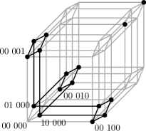
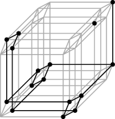
?figurename? 1: An example for the transformation. Left: $\psi=\left(x_{1}\vee\overline{x_{2}}\right)\wedge\left(\overline{x_{1}}\vee x_{2}\right)$, center: $T_{\psi}^{\sim}$, right: $T_{\psi}$. The “axis vertices” are labeled in the first two graphs.

Now $G(T_{\psi})$ is connected iff $G(\psi)$ is connected.

Step 2. Again, we use the algorithm Tr from the previous proof to transform any 1-reproducing 3-CNF-formula $\phi$ into a $B$-formula $\phi^{\prime}$ equivalent to $T_{\phi}$, but with the definition (4) of $T$. Again, we have to show $T_{\wedge}(T_{\psi_{1}},T_{\psi_{2}})\equiv T_{\psi_{1}\wedge\psi_{2}}$. Here,

$$T_{\wedge}(T_{\psi_{1}},T_{\psi_{2}}) = \left(T_{\psi_{1}}\wedge T_{\psi_{2}}\wedge(\boldsymbol{y}=\boldsymbol{1})\right)\vee\left(\overline{\overline{T_{\psi_{1}}}\wedge\overline{T_{\psi_{2}}}}\wedge(\boldsymbol{y}=\boldsymbol{0})\right)$$

$$\vee\left(\boldsymbol{y}\in\left\{100,010,001\right\}\wedge\neg\left(\overline{T_{\psi_{1}}}\wedge\overline{T_{\psi_{2}}}\wedge(\boldsymbol{y}=001)\right)\right)$$

$$\vee\left(T_{\psi_{1}}\wedge T_{\psi_{2}}\wedge(\boldsymbol{y}=110)\right).$$

We consider the parts of the formula in turn: For any formula $\xi$ we have $T_{\xi}(\boldsymbol{x}_{\xi})\wedge(\boldsymbol{y}=\boldsymbol{1})\equiv\xi(\boldsymbol{x}_{\xi})\wedge(\boldsymbol{y}=\boldsymbol{1})$ and $T_{\xi}(\boldsymbol{x}_{\xi})\wedge(\boldsymbol{y}=\boldsymbol{0})\equiv\overline{\psi(\overline{\boldsymbol{x}_{\xi}})}\wedge(\boldsymbol{y}=\boldsymbol{0})$, where $\boldsymbol{x}_{\xi}$ denotes the variables of $\xi$. Using $\overline{\overline{T_{\psi_{1}}(\boldsymbol{x}_{\psi_{1}})}\wedge\overline{T_{\psi_{2}}(\boldsymbol{x}_{\psi_{2}})}}\wedge(\boldsymbol{y}=\boldsymbol{0})=\left(T_{\psi_{1}}(\boldsymbol{x}_{\psi_{1}})\vee T_{\psi_{2}}(\boldsymbol{x}_{\psi_{2}})\right)\wedge(\boldsymbol{y}=\boldsymbol{0})$, the first line becomes

$$\left(\psi_{1}(\boldsymbol{x}_{\psi_{1}})\wedge\psi_{2}(\boldsymbol{x}_{\psi_{2}})\wedge(\boldsymbol{y}=\boldsymbol{1})\right)\vee\left(\left(\overline{\psi_{1}(\overline{\boldsymbol{x}_{\psi_{1}}})\wedge\psi_{2}(\overline{\boldsymbol{x}_{\psi_{2}}})}\right)\wedge(\boldsymbol{y}=\boldsymbol{0})\right).$$

For the second line, we observe

$$\overline{T_{\psi}(\boldsymbol{x}_{\psi})} \equiv \left(\overline{\psi(\boldsymbol{x}_{\psi})}\vee\neg(\boldsymbol{y}=\boldsymbol{1})\right)\wedge\left(\psi(\boldsymbol{\overline{x}_{\psi}})\vee\neg(\boldsymbol{y}=\boldsymbol{0})\right)$$

$$\wedge\left(\boldsymbol{y}\notin\left\{100,010,001\right\}\vee\left((\boldsymbol{x}_{\psi}=\boldsymbol{0})\wedge(\boldsymbol{y}=001)\right)\right)$$

$$\wedge(\neg(\boldsymbol{x}_{\psi}=\boldsymbol{1})\vee\overline{(\boldsymbol{y}=110)}),$$

thus $\overline{T_{\psi}(\boldsymbol{x}_{\psi})}\wedge(\boldsymbol{y}=001)\equiv(\boldsymbol{x}_{\psi}=\boldsymbol{0})\wedge(\boldsymbol{y}=001)$, and the second line becomes

$$\vee\left(\boldsymbol{y}\in\left\{100,010,001\right\}\wedge\neg\left((\boldsymbol{x}_{\psi_{1}}=\boldsymbol{0})\wedge(\boldsymbol{x}_{\psi_{2}}=\boldsymbol{0})\wedge(\boldsymbol{y}=001)\right)\right).$$

Since $T_{\psi}(\boldsymbol{x}_{\psi})\wedge(\boldsymbol{y}=110)\equiv(\boldsymbol{x}_{\psi}=\boldsymbol{1})\wedge(\boldsymbol{y}=110)$ for any $\psi$, the third line becomes

$$\vee\left((\boldsymbol{x}_{\psi_{1}}=\boldsymbol{1})\wedge(\boldsymbol{x}_{\psi_{2}}=\boldsymbol{1})\wedge(\boldsymbol{y}=110)\right).$$

Now $T_{\wedge}(T_{\psi_{1}},T_{\psi_{2}})$ equals

$$T_{\psi_{1}\wedge\psi_{2}} = \left(\psi_{1}(\boldsymbol{x}_{\psi_{1}})\wedge\psi_{2}(\boldsymbol{x}_{\psi_{2}})\wedge(\boldsymbol{y}=\boldsymbol{1})\right)\vee\left(\overline{\psi_{1}(\overline{\boldsymbol{x}_{\psi_{1}}})\wedge\psi_{2}(\overline{\boldsymbol{x}_{\psi_{2}}})}\wedge(\boldsymbol{y}=\boldsymbol{0})\right)$$

$$\vee\left(\boldsymbol{y}\in\left\{100,010,001\right\}\wedge\neg\left((\boldsymbol{x}_{\psi_{1}}=\boldsymbol{0})\wedge(\boldsymbol{x}_{\psi_{2}}=\boldsymbol{0})\wedge(\boldsymbol{y}=001)\right)\right)$$

$$\vee\left((\boldsymbol{x}_{\psi_{1}}=\boldsymbol{1})\wedge(\boldsymbol{x}_{\psi_{2}}=\boldsymbol{1})\wedge(\boldsymbol{y}=110)\right).$$

2. This follows from 1. by Proposition 3.1.

3. By Lemma 3.2 there is an 1-reproducing $(n-3)$-ary function $f$ with diameter of at least $2^{\left\lfloor\frac{n-3}{2}\right\rfloor}$. Let $f$ be represented by a formula $\phi$; then, $T_{\phi}$ represents an $n$-ary function of the same diameter in $\mathsf{D}_{1}$.∎

Lemma 4.6.

If $[B]\supseteq\mathsf{S}_{02}^{k}$ for any $k\geq 2$,

1. st-BF-Conn($B$) and BF-Conn($B$) are $\mathrm{PSPACE}$-complete,

2. st-Circ-Conn($B$) and Circ-Conn($B$) are $\mathrm{PSPACE}$-complete,

3. for $n\geq k+4$, there is an $n$-ary function $f\in[B]$ with diameter of at least $2^{\left\lfloor\frac{n-k-2}{2}\right\rfloor}$.

?proofname?.

1. Step 1. Since $\mathsf{S}_{02}^{k}=\mathsf{S}_{0}^{k}\cap\mathsf{R}_{0}\cap\mathsf{R}_{1}$, $T_{\psi}$ must be 0-separating of degree $k$, 0-reproducing, and 1-reproducing. As in the previous proof, we construct an intermediate formula $T_{\psi}^{\sim}$. For $\psi(\boldsymbol{x})$, let

$$T_{\psi}^{\sim}=\left(\psi\wedge y\wedge(\boldsymbol{z}=\boldsymbol{0})\right)\vee(|\boldsymbol{z}|>1),$$

where $y$ and $\boldsymbol{z}=(z_{1},\ldots,z_{k+1})$ are new variables.

$T_{\psi}^{\sim}(\boldsymbol{x},y,\boldsymbol{z})$ is 0-separating of degree $k$, since all vectors that are no solutions of $T_{\psi}^{\sim}$ have $|\boldsymbol{z}|\leq 1$, i.e. $\boldsymbol{z}\in\left\{0\cdots 0,10\cdots 0,010\cdots 0,\ldots,0\cdots 01\right\}\subset\{0,1\}^{k+1}$, and thus any $k$ of them have at least one common variable assigned 0. Also, $T_{\psi}^{\sim}$ is 0-reproducing and still 1-reproducing.

Further, for any two solutions $\boldsymbol{s}$ and $\boldsymbol{t}$ of $\psi(\boldsymbol{x})$, $\boldsymbol{s}^{\prime}=\boldsymbol{s}\cdot 1\cdot 0\cdots 0$ and $\boldsymbol{t}^{\prime}=\boldsymbol{t}\cdot 1\cdot 0\cdots 0$ are solutions of $T_{\psi}^{\sim}(\boldsymbol{x},y,\boldsymbol{z})$ and are connected in $G(T_{\psi}^{\sim})$ iff $\boldsymbol{s}$ and $\boldsymbol{t}$ are connected in $G(\psi)$.

But again, we have produced an additional connected component (consisting of all solutions with $|\boldsymbol{z}|>1$). To connect it to a component corresponding to one of $\psi$, we add $1\cdots 1\cdot 1\cdot 10\cdots 0$ as a solution,

$$T_{\psi} = \left(\psi\wedge y\wedge(\boldsymbol{z}=\boldsymbol{0})\right)\vee(|\boldsymbol{z}|>1)\vee\left((\boldsymbol{x}=\boldsymbol{1})\wedge y\wedge(\boldsymbol{z}=10\cdots 0)\right).$$

Now $G(T_{\psi})$ is connected iff $G(\psi)$ is connected.

Step 2. Again we show that the algorithm Tr works in this case. Here,

$$T_{\wedge}(T_{\psi_{1}},T_{\psi_{2}}) = \left(T_{\psi_{1}}(\boldsymbol{x}_{\psi_{1}})\wedge T_{\psi_{2}}(\boldsymbol{x}_{\psi_{2}})\wedge y\wedge(\boldsymbol{z}=\boldsymbol{0})\right)\vee(|\boldsymbol{z}|>1)$$

$$\vee\left(T_{\psi_{1}}(\boldsymbol{x}_{\psi_{1}})\wedge T_{\psi_{2}}(\boldsymbol{x}_{\psi_{2}})\wedge y\wedge(\boldsymbol{z}=10\cdots 0)\right).$$

Since $T_{\psi}(\boldsymbol{x}_{\psi})\wedge y\wedge(\boldsymbol{z}=\boldsymbol{0})\equiv\psi(\boldsymbol{x}_{\psi})\wedge y\wedge(\boldsymbol{z}=\boldsymbol{0})$ and $T_{\psi}(\boldsymbol{x}_{\psi})\wedge y\wedge(\boldsymbol{z}=10\cdots 0)\equiv(\boldsymbol{x}_{\psi}=1)\wedge y\wedge(\boldsymbol{z}=10\cdots 0)$ for any $\psi$, this is equivalent to

$$T_{\psi_{1}\wedge\psi_{2}} = \left(\psi_{1}(\boldsymbol{x}_{\psi_{1}})\wedge\psi_{2}(\boldsymbol{x}_{\psi_{2}})\wedge y\wedge(\boldsymbol{z}=\boldsymbol{0})\right)\vee(|\boldsymbol{z}|>1)$$

$$\vee\left(\boldsymbol{x}_{\psi_{1}}\wedge\boldsymbol{x}_{\psi_{2}}\wedge y\wedge(\boldsymbol{z}=10\cdots 0)\right).$$

2. This follows from 1. by Proposition 3.1.

3. By Lemma 3.2 there is an 1-reproducing $(n-k-2)$-ary function $f$ with diameter of at least $2^{\left\lfloor\frac{n-k-2}{2}\right\rfloor}$. Let $f$ be represented by a formula $\phi$; then, $T_{\phi}$ represents an $n$-ary function of the same diameter in $\mathsf{S}_{02}^{k}$. ∎

This completes the proof of Theorem 2.1.

5 Quantified Formulas

Definition 5.1.

A quantified $B$-formula $\phi$ (in prenex normal form) is an expression of the form

$$Q_{1}y_{1}\cdots Q_{m}y_{m}\varphi(y_{1},\ldots,y_{m},x_{1},\ldots,x_{n}),$$

where $\varphi$ is a $B$-formula, and $Q_{1},\ldots,Q_{m}\in\{\exists,\forall\}$ are quantifiers. We denote the corresponding connectivity resp. $st$-connectivity problems by QBF-Conn($B$) resp. st-QBF-Conn($B$).

Theorem 5.2.

Let $B$ be a finite set of Boolean functions.

1. If $B\subseteq\mathsf{M}$ or $B\subseteq\mathsf{L}$, then

   1. st-QBF-Conn($B$) and QBF-Conn($B$) are in P,

   2. the diameter of every quantified $B$-formula is linear in the number of free variables.

2. Otherwise,

   1. st-QBF-Conn($B$) and QBF-Conn($B$) are $\mathrm{PSPACE}$-complete,

   2. there are quantified $B$-formulas with at most one quantifier such that their diameter is exponential in the number of free variables.

?proofname?.

1. For $B\subseteq\mathsf{M}$, any quantified $B$-formula $\phi$ represents a monotone function: Using $\exists y\psi(y,\boldsymbol{x})=\psi(0,\boldsymbol{x})\vee\psi(1,\boldsymbol{x})$ and $\forall y\psi(y,\boldsymbol{x})=\psi(0,\boldsymbol{x})\wedge\psi(1,\boldsymbol{x})$ recursively, we can transform $\phi$ into an equivalent $\mathsf{M}$-formula since $\wedge$ and $\vee$ are monotone. Thus as in Lemma 3.2, st-QBF-Conn($B$) and QBF-Conn($B$) are trivial, and $d_{f}(\boldsymbol{a},\boldsymbol{b})=|\boldsymbol{a}-\boldsymbol{b}|$ for any two solutions $\boldsymbol{a}$ and $\boldsymbol{b}$.

For a quantified $B$-formula $\phi=Q_{1}y_{1}\cdots Q_{m}y_{m}\varphi$ with $B\subseteq\mathsf{L}$, we first remove the quantifications over all fictive variables of $\varphi$ (and eliminate the fictive variables if necessary). If quantifiers remain, $\phi$ is either tautological (if the rightmost quantifier is $\exists$) or unsatisfiable (if the rightmost quantifier is $\forall$), so the problems are trivial, and $d_{f}(\boldsymbol{a},\boldsymbol{b})=|\boldsymbol{a}-\boldsymbol{b}|$ for any two solutions $\boldsymbol{a}$ and $\boldsymbol{b}$. Otherwise, we have a quantifier-free formula and the statements follow from Lemma 3.4.

2. Again as in Lemma 3.1, it follows that st-QBF-Conn($B$) and QBF-Conn($B$) are in $\mathrm{PSPACE}$, since the evaluation problem for quantified $B$-formulas is in $\mathrm{PSPACE}$ [32].

An inspection of Post’s lattice shows that if $B\nsubseteq\mathsf{M}$ and $B\nsubseteq\mathsf{L}$, then $[B]\supseteq\mathsf{S}_{12}$, $[B]\supseteq\mathsf{D}_{1}$, or $[B]\supseteq\mathsf{S}_{02}$, so we have to prove $\mathrm{PSPACE}$-completeness and show the existence of $B$-formulas with an exponential diameter in these cases.

For $[B]\supseteq\mathsf{S}_{12}$ and $[B]\supseteq\mathsf{D}_{1}$, the statements for the $\mathrm{PSPACE}$-hardness and the diameter obviously carry over from Theorem 2.1.

For $B\supseteq\mathsf{S}_{02}$, we give a reduction from the problems for (unquantified) 3-CNF-formulas; we proceeded again similar as in the proof of Lemma 4.4. We give a transformation $T_{\psi}$ s.t. $T_{\psi}\in\mathsf{S}_{02}$ for all formulas $\psi$. Since $\mathsf{S}_{02}=\mathsf{S}_{0}\cap\mathsf{R}_{0}\cap\mathsf{R}_{1}$, $T_{\psi}$ must be self-dual, 0-reproducing, and 1-reproducing. For $\psi(\boldsymbol{x})$ let

$$T_{\psi}=(\psi\wedge y)\vee z,$$

with the two new variables $y$ and $z$.

$T_{\psi}$ is 0-separating since all vectors that are no solutions have $z=0$. Also, $T_{\psi}$ is 0-reproducing and 1-reproducing. Again, we use the algorithm Tr from the proof of Lemma 4.4 to transform any 3-CNF-formula $\phi$ into a $B$-formula $\varphi^{\prime}$ equivalent to $T_{\phi}$. Again, we show

$$T_{\wedge}(T_{\psi_{1}},T_{\psi_{2}}) = \left(\left((\psi_{1}\wedge y)\vee z\right)\wedge\left((\psi_{2}\wedge y)\vee z\right)\wedge y\right)\vee z$$

$$\equiv \left(\left(\psi_{1}\wedge y\right)\wedge\left(\psi_{2}\wedge y\right)\wedge y\right)\vee z$$

$$\equiv \left(\psi_{1}\wedge\psi_{2}\wedge y\right)\vee z=T_{\psi_{1}\wedge\psi_{2}}.$$

Now let

$$\phi^{\prime}=\forall z\varphi^{\prime}.$$

Then, for any two solutions $\boldsymbol{s}$ and $\boldsymbol{t}$ of $\phi(\boldsymbol{x})$, $\boldsymbol{s}^{\prime}=\boldsymbol{s}\cdot 1$ and $\boldsymbol{t}^{\prime}=\boldsymbol{t}\cdot 1$ are solutions of $\phi^{\prime}(\boldsymbol{x},y)$, and they are connected in $G(\phi^{\prime})$ iff $\boldsymbol{s}$ and $\boldsymbol{t}$ are connected in $G(\phi)$, and $G(\phi^{\prime})$ is connected iff $G(\phi)$ is connected.

The proof of Lemma 3.2 shows that there is an $(n-1)$-ary function $f$ with diameter of at least $2^{\left\lfloor\frac{n-1}{2}\right\rfloor}$. Let $f$ be represented by a formula $\phi$; then $\phi^{\prime}$ as defined above is a quantified $B$-formula with $n$ free variables and one quantifier with the same diameter.∎

Remark 5.3.

An analog to Theorem 5.2 also holds for quantified circuits as defined in [31, Section 7].

?chaptername? 4 Future Directions

We have proved classifications in two quite different settings: In Schaefer’s framework for constraint satisfaction problems, specifically CNF_C($\mathcal{S}$)-formulas, CNF($\mathcal{S}$)-formulas and Q-CNF_C($\mathcal{S}$)-formulas, and in Post’s framework for nested formulas and circuits, specifically $B$-formulas, $B$-circuits, and quantified $B$-formulas.

While we now have a quite complete picture for nested formulas and circuits, and also for CNF_C($\mathcal{S}$)-formulas and Q-CNF_C($\mathcal{S}$)-formulas, the complexity of the connectivity problem for CNF($\mathcal{S}$)-formulas without constants is still open for sets $\mathcal{S}$ that are 0-valid, 1-valid, or complementive, but not Schaefer, nor nc-CPSS, nor quasi disconnecting.

Recently, Scharpfenecker refined some of our complexity results for CNF_C($\mathcal{S}$)-formulas up to logarithmic-space isomorphisms and investigated the realizable solution-graphs in more detail [37].

It seems very likely that connectivity is not for all these sets in P, since there are even Schaefer sets that are 0-valid or 1-valid, but have a coNP-complete connectivity problem. On the other hand, it seems promising to search for more nc-CPS sets, for which we have a P or $\mathrm{P^{NP}}$ algorithm.

Also, one might further explore the connection between the connectivity of CNF-formulas and properties of the corresponding hypergraphs (see Remark 7.3); while we used this connection only for Horn formulas and thus dealt with hypergraphs of head-size 1, there might be useful reductions between the connectivity problems for more general CNF-formulas and problems for the corresponding hypergraphs.

There is a multitude of interesting variations of the problems investigated in this thesis, in different directions; we close with a quick survey of some such variations.

• Other representations of Boolean relations  Disjunctive normal forms with special connectivity properties were studied by Ekin et al. already in 1997 for their “important role in problems appearing in various areas including in particular discrete optimization, machine learning, automated reasoning, etc.” [15].
      There are yet more kinds of representations for Boolean relations, such as binary decision diagrams and Boolean neural networks, and investigating the connectivity in these settings might be worthwhile as well.

• Related problems  Other connectivity-related problems already mentioned by Gopalan et al. are counting the number of components and approximating the diameter. For counting the number of components, Gopalan et al. mentioned in [18] that they could show that the problem is in P for affine, monotone and dual-monotone relations, and #P-complete otherwise.
      Further, especially with regard to reconfiguration problems, it is interesting to find the shortest path between two solutions; this was recently investigated by Mouawad et al. [27], who proved a computational trichotomy for this problem. In this direction, one could also consider the optimal path according to some other measure.

• Other definitions of connectivity  Our definition of connectivity is not the only sensible one: One could regard two solutions connected whenever their Hamming distance is at most $d$, for some $d\geq 1$; this was already considered related to random satisfiability, see [3]. This generalization seems meaningful as well as challenging.

• Higher domains  Finally, a most interesting subject are CSPs over larger domains; in 1993, Feder and Vardi conjectured a dichotomy for the satisfiability problem over arbitrary finite domains [17], and while the conjecture was proved for domains of size three in 2002 by Bulatov [9], it remains open to date for the general case. Close investigation of the solution space might lead to valuable insights here.
      For $k$-colorability, which is a special case of the general CSP over a $k$-element set, the connectivity problems and the diameter were already studied by Bonsma and Cereceda [6], and Cereceda, van den Heuvel, and Johnson [14]. They showed that for $k=3$ the diameter is at most quadratic in the number of vertices and the $st$-connectivity problem is in P, while for $k\geq 4$, the diameter can be exponential and $st$-connectivity is PSPACE-complete in general.