Partitioning Data on Features or Samples in Communication-Efficient Distributed Optimization?

Abstract

In this paper we study the effect of the way that the data is partitioned in distributed optimization. The original DiSCO algorithm [Communication-Efficient Distributed Optimization of Self-Concordant Empirical Loss, Yuchen Zhang and Lin Xiao, 2015] partitions the input data based on samples. We describe how the original algorithm has to be modified to allow partitioning on features and show its efficiency both in theory and also in practice.

1 Introduction

As the size of the datasets becomes larger and larger, distributed optimization methods for machine learning have become increasingly important [2, 5, 13]. Existing mehods often require a large amount of communication between computing nodes [17, 7, 9, 18], which is typically several magnitudes slower than reading data from their own memory [10]. Thus, distributed machine learning suffers from the communication bottleneck on real world applications.

In this paper we focus on the regularized empirical risk minimization problem. Suppose we have $n$ data samples $\{x_{i},y_{i}\}_{i=1}^{n}$, where each $x_{i}\in\mathbb{R}^{d}$ (i.e. we have $d$ features), $y_{i}\in\mathbb{R}$. We will denote by $X:=[x_{1},...,x_{n}]\in\mathbb{R}^{d\times n}$. The optimization problem is to minimize the regularized empirical loss (ERM)

$$f(w):=\frac{1}{n}\sum_{i=1}^{n}\phi_{i}(w,x_{i})+\frac{\lambda}{2}\|w\|_{2}^{2},$$ (1)

where the first part is the data fitting term, $\phi:\mathbb{R}^{d}\times\mathbb{R}^{d}\rightarrow\mathbb{R}$ is a loss function which typically depends on $y_{i}$. Some popular loss functions includes hinge loss $\phi_{i}(w,x_{i})=\max\{0,1-y_{i}w^{T}x_{i}\}$, square loss $\phi_{i}(w,x_{i})=(y_{i}-w^{T}x_{i})^{2}$ or logistic loss $\phi_{i}(w,x_{i})=\log(1+\exp(-y_{i}w^{T}x_{i}))$. The second part of objective function (1) is $\ell_{2}$ regularizer ($\lambda>0$) which helps to prevent over-fitting of the data.

We assume that the loss function $\phi_{i}$ is convex and self-concordant [19]:

Assumption 1.

For all $i\in[n]:=\{1,2,\dots,n\}$ the convex function $\phi$ is self-concordant with parameter $M$ i.e. the following inequality holds:

$$|u^{T}(f^{\prime\prime\prime}(w)[u])u|\leq M(u^{T}f^{\prime\prime}(w)u)^{\frac{3}{2}}$$ (2)

for any $u\in\mathbb{R}^{d}$ and $w\in dom(f)$, where $f^{\prime\prime\prime}(w)[u]:=\lim_{t\rightarrow 0}\frac{1}{t}(f^{\prime\prime}(w+tu)-f^{\prime\prime}(w))$.

There has been an enormous interest in large-scale machine learning problems and many parallel [4, 11] or distributed algorithms have been proposed [1, 16, 12, 14, 8].

The main bottleneck in distributed computing –communication– was handled by many researches differently. Some work considered ADMM type methods [3, 6], another used block-coordinate type algorithms [8, 17, 7, 9], where they tried to solve the local sub-problems more accurately (which should decrease the overall communications requirements when compared with more basic approaches [15, 16]).

2 Algorithm

Algorithm 1 High-level DiSCO algorithm

1:  Input: parameters $\rho,\mu\geq 0$, number of iterations $K$

2:  Initializing $w_{0}$.

3:  for k = 0,1,2,…,K do

4:     Option 1: Given $w_{k}$, run DiSCO-S PCG Algorithm 2, get $v_{k}$ and $\delta_{k}$

5:     Option 2: Given $w_{k}$, run DiSCO-F PCG Algorithm 3, get $v_{k}$ and $\delta_{k}$

6:     Update $w_{k+1}=w_{k}-\frac{1}{1+\delta_{k}}v_{k}$

7:  end for

8:  Output: $w_{K+1}$

We assume that we have $m$ machines (computing nodes) available which can communicate between each other over the network. We assume that the space needed to store the data matrix $X$ exceeds the memory of every single node. Thus we have to split the data (matrix $X$) over the $m$ nodes. The natural question is: How to split the data into $m$ parts? There are many possible ways, but two obvious ones:

1. split the data matrix $X$ by rows (i.e. create $m$ blocks by rows); Because rows of $X$ corresponds to features, we will denote the algorithm which is using this type of partitioning as DiSCO-F;

2. split the data matrix $X$ by columns; Let us note that columns of $X$ corresponds to samples we will denote the algorithm which is using this type of partitioning as DiSCO-S;

Notice that the DiSCO-S is exactly the same as DiSCO proposed and analyzed in [19]. In each iteration of Algorithm 1, wee need to compute an inexact Newton step $v_{k}$ such that $\|f^{\prime\prime}(w_{k})v_{k}-f^{\prime}(w_{k})\|_{2}\leq\epsilon_{k}$, which is an approximate solution to the Newton system $f^{\prime\prime}(w_{k})v_{k}=\nabla f(w_{k})$. The discussion about how to choose $\epsilon_{k}$ and $K$ and a convergence guarantees for Algorithm 1 can be found in [19]. The main goal of this work is to analyze the algorithmic modifications to DiSCO-S when the partitioning type is changed. It will turn out that partitioning on features (DiSCO-F) can lead to algorithm which uses less communications (depending on the relations between $d$ and $n$) (see Section 3).

Algorithm 2 Distributed DiSCO-S: PCG algorithm – data partitioned by samples

1:  Input: $w_{k}\in\mathbb{R}^{d}$, and $\mu\geq 0$.communication (Broadcast $w_{k}\in\mathbb{R}^{d}$ and reduceAll $\nabla f_{i}(w_{k})\in\mathbb{R}^{d}$ )

2:  Initialization: Let $P$ be computed as (4). $v_{0}=0$, $s_{0}=P^{-1}r_{0}$, $r_{0}=\nabla f(w_{k})$, $u_{0}=s_{0}$.

3:  for $t=0,1,2,...$ do

4:     Compute $Hu_{t}$ communication (Broadcast $u_{t}\in\mathbb{R}^{d}$ and reduceAll $f{{}^{\prime\prime}}_{i}(w_{k})u_{t}\in\mathbb{R}^{d}$ )

5:     Compute $\alpha_{t}=\frac{\langle r_{t},s_{t}\rangle}{\langle u_{t},Hu_{t}\rangle}$

6:     Update $v_{(t+1)}=v_{t}+\alpha_{t}u_{t},Hv_{(t+1)}=Hv_{t}+\alpha_{t}Hu_{t},r_{t+1}=r_{t}-\alpha_{t}Hu_{t}$.

7:     Update $s_{(t+1)}=P^{-1}r_{(t+1)}$.

8:     Compute $\beta_{t}=\frac{\langle r_{(t+1)},s_{(t+1)}\rangle}{\langle r_{t},s_{t}\rangle}$

9:     Update $u_{(t+1)}=s_{(t+1)}+\beta_{t}u_{t}$.

10:     until: $\|r_{(r+1)}\|_{2}\leq\epsilon_{k}$

11:  end for

12:  Return: $v_{k}=v_{t+1}$, $\delta_{k}=\sqrt{v_{(t+1)}^{T}Hv_{t}+\alpha_{t}v_{(t+1)}^{T}Hu_{t}}$

DiSCO-S Algorithm.

If the dataset is partitioned by samples, such that $j$–th node will only store $X_{j}=[x_{j,1},...,x_{j,n_{j}}]\in\mathbb{R}^{d\times n_{j}}$, which is a part of $X$, then each machine can evaluate a local empirical loss function

$$f_{j}(w):=\frac{1}{n_{j}}\sum_{i=1}^{n_{j}}\phi(w,x_{j,i})+\frac{\lambda}{2}\|w\|_{2}^{2}.$$ (3)

Because $\{X_{j}\}$ is a partition of $X$ we have $\sum_{j=1}^{m}n_{j}=n$, our goal now becomes to minimize the function $f(w)=\frac{1}{m}\sum_{h=1}^{m}f_{j}(w)$. Let $H$ denote the Hessian $f^{\prime\prime}(w_{k})$. For simplicity in this paper we consider only square loss and hence in this case $f^{\prime\prime}(w_{k})$ is constant (independent on $w_{k}$).

In Algorithm 2, each machine will use its local data to compute the local gradient and local Hessian and then aggregate them together. We also have to choose one machine as the master, which computes all the vector operations of PCG loops (Preconditioned Conjugate Gradient), i.e., step 5-9 in Algorithm 2.

The preconditioning matrix for PCG is defined only on master node and consists of the local Hessian approximated by a subset of data available on master node with size $\tau$, i.e.

$$P=\frac{1}{\tau}\sum_{j=1}^{\tau}\phi^{{}^{\prime\prime}}(w,x_{1,j})+\mu I,$$ (4)

where $\mu$ is a small regularization parameter. Algorithm 2 presents the distributed PCG mathod for solving the preconditioning linear system

$$P^{-1}Hv_{k}=P^{-1}\nabla f(w_{k}).$$ (5)

DiSCO-F Algorithm.

If the dataset is partitioned by features, then $j$th machine will store $X_{j}=[a_{1}^{[j]},...,a_{n}^{[j]}]\in\mathbb{R}^{d_{j}\times n}$, which contains all the samples, but only with a subset of features. Also, each machine will only store $w_{k}^{[j]}\in\mathbb{R}^{d_{j}}$ and thus only be responsible for the computation and updates of $\mathbb{R}^{d_{j}}$ vectors. By doing so, we only need one ReduceAll on a vector of length $n$, in addition to two ReduceAll on scalars number.

Algorithm 3 Distributed DiSCO-F: PCG algorithm – data partitioned by features

1:  Input: $w_{k}^{[i]}\in\mathbb{R}^{d_{i}}$ for $i=1,2,...,m$, and $\mu\geq 0$.

2:  Initialization: Let $P$ be computed as (4). $v_{0}^{[i]}=0$, $s_{0}^{[i]}={(P^{-1})}^{[i]}r_{0}^{[i]}$, $r_{0}^{[i]}=f^{\prime}(w_{k}^{[i]})$, $u_{0}^{[i]}=s_{0}^{[i]}$.

3:  while $\|r_{r+1}\|_{2}\leq\epsilon_{k}$ do

4:     Compute $(Hu_{t})^{[i]}$. communication (ReduceAll an $\mathbb{R}^{d_{i}}$ vector)

5:     Compute $\alpha_{t}=\frac{\sum_{i=1}^{m}\langle r_{t}^{[i]},s_{t}^{[i]}\rangle}{\sum_{i=1}^{m}\langle u_{t}^{[i]},(Hu_{t})^{[i]}\rangle}$. communication (ReduceAll a number)

6:     Update $v_{t+1}^{[i]}=v_{t}^{[i]}+\alpha_{t}u_{t}^{[i]},(Hv_{t+1})^{[i]}=(Hv_{t})^{[i]}+\alpha_{t}(Hu_{t})^{[i]},r_{t+1}^{[i]}=r_{t}^{[i]}-\alpha_{t}(Hu_{t})^{[i]}$.

7:     Update $s_{t+1}^{[i]}=(P^{-1})^{[i]}r_{t+1}^{[i]}$.

8:     Compute $\beta_{t}=\frac{\sum_{i=1}^{m}\langle r_{t+1}^{[i]},s_{t+1}^{[i]}\rangle}{\sum_{i=1}^{m}\langle r_{t}^{[i]},s_{t}^{[i]}\rangle}$. communication (ReduceAll a number)

9:     Update $u_{t+1}^{[i]}=s_{t+1}^{[i]}+\beta_{t}u_{t}^{[i]}$.

10:  end while

11:  Compute $\delta_{k}^{[i]}=\sqrt{{v_{t+1}^{[i]}}^{T}(Hv_{t})^{[i]}+\alpha_{t}{v_{t+1}^{[i]}}^{T}(Hu_{t})^{[i]}}$.

12:  Integration: $v_{k}=[v_{t+1}^{[1]},...,v_{t+1}^{[m]}]$, $\delta_{k}=[\delta_{t+1}^{[1]},...,\delta_{t+1}^{[m]}]$ communication (Reduce an $\mathbb{R}^{d_{i}}$ vector)

13:  Return: $v_{k}$, $\delta_{k}$

Comparison of Communication and Computational Cost.

In Table 1 we compare the communication cost for the two approaches DiSCO-S/DiSCO-F. As it is obvious from the table, DiSCO-F requires only one reduceAll of a vector of length $n$, whereas the DiSCO-S needs one reduceAll of a vector of length $d$ and one broadcast of vector of size $d$. So roughly speaking, when $n<d$ then DiSCO-F will need less communication. However, very interestingly, the advantage of DiSCO-F is the fact that it uses CPU on every node more effectively. It also requires less total amount of work to be performed on each node, leading to more balanced and efficient utilization of nodes.

Table 1: Comparison of computation and communication between different ways of partition on data.

			partition by samples	partition by features
computation	master	matrix-vector multiplication	$1(\mathbb{R}^{d\times d}\times\mathbb{R}^{d})$	$1(\mathbb{R}^{d_{1}\times d_{1}}\times\mathbb{R}^{d_{1}})$
		back solving linear system	1 ($\mathbb{R}^{d}$)	1 $(\mathbb{R}^{d_{1}})$
		sum of vectors	4 ($\mathbb{R}^{d}$)	4 ($\mathbb{R}^{d_{1}}$)
		inner product of vectors	4 ($\mathbb{R}^{d}$)	4 ($\mathbb{R}^{d_{1}}$)
	nodes	matrix-vector multiplication	1 $(\mathbb{R}^{d\times d}\times\mathbb{R}^{d})$	$1(\mathbb{R}^{d_{1}\times d_{i}}\times\mathbb{R}^{d_{i}})$
		back solving linear system	0	1 $(\mathbb{R}^{d_{i}})$
		sum of vectors	0	4 $(\mathbb{R}^{d_{i}})$
		inner product of vectors	0	4 $(\mathbb{R}^{d_{i}})$
communication	Broadcast		one $\mathbb{R}^{d}$ vector	0
	ReduceAll		one $\mathbb{R}^{d}$ vector	one $\mathbb{R}^{n}$ vector, 2 $\mathbb{R}^{1}$

3 Numerical Experiments

We present experiments on several standard large real-world datasets: news20.binary $(d=1,355,191;n=19,996;0.13GB)$; kdd2010(test) $(d=29,890,095;n=748,401;0.19GB)$; and epsilon $(d=2,000;n=100,000;3.04GB)$. Each data was split into $m$ machines. We implement DiSCO-S, DiSCO-F and CoCoA+ [9] algorithms for comparison in C++, and run them on the Amazon cloud, using 4 m3.xlarge EC2 instances. Figure 1 compares the evolution of $\|\nabla f(w)\|$ as function of elapsed time, number of communications and iterations. As it can be observed, the DiSCO-F needs almost the same number of iterations as DiSCO-S, however, it needs roughly just half the communication, therefore it is much faster (if we care about elapsed time).

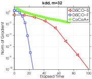
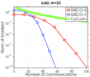
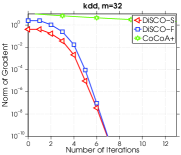
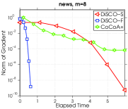
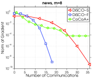
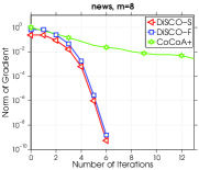
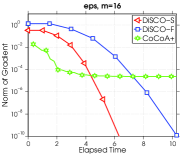
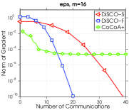
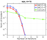
Figure 1: Comparison of DiSCO-S, DiSCO-F and CoCoA+ on various datasets.

References

• [1] Alekh Agarwal and Johnย C Duchi. Distributed delayed stochastic optimization. In Advances in Neural Information Processing Systems, pages 873โ€“881, 2011.
• [2] Dimitriย P Bertsekas and Johnย N Tsitsiklis. Parallel and distributed computation: numerical methods. Prentice-Hall, Inc., 1989.
• [3] Stephen Boyd, Neal Parikh, Eric Chu, Borja Peleato, and Jonathan Eckstein. Distributed optimization and statistical learning via the alternating direction method of multipliers. Foundations and Trendsยฎ in Machine Learning, 3(1):1โ€“122, 2011.
• [4] Josephย K Bradley, Aapo Kyrola, Danny Bickson, and Carlos Guestrin. Parallel coordinate descent for l1-regularized loss minimization. arXiv preprint arXiv:1105.5379, 2011.
• [5] Ofer Dekel, Ran Gilad-Bachrach, Ohad Shamir, and Lin Xiao. Optimal distributed online prediction using mini-batches. The Journal of Machine Learning Research, 13(1):165โ€“202, 2012.
• [6] Wei Deng and Wotao Yin. On the global and linear convergence of the generalized alternating direction method of multipliers. Journal of Scientific Computing, pages 1โ€“28, 2012.
• [7] Martin Jaggi, Virginia Smith, Martin Takรกc, Jonathan Terhorst, Sanjay Krishnan, Thomas Hofmann, and Michaelย I Jordan. Communication-efficient distributed dual coordinate ascent. In Advances in Neural Information Processing Systems, pages 3068โ€“3076, 2014.
• [8] Ching-Pei Lee and Dan Roth. Distributed box-constrained quadratic optimization for dual linear SVM. ICML, 2015.
• [9] Chenxin Ma, Virginia Smith, Martin Jaggi, Michaelย I Jordan, Peter Richtรกrik, and Martin Takรกฤ. Adding vs. averaging in distributed primal-dual optimization. In ICML 2015 - Proceedings of the 32th International Conference on Machine Learning, volumeย 37, pages 1973โ€“1982. JMLR, 2015.
• [10] Jakub Marecek, Peter Richtรกrik, and Martin Takรกc. Distributed block coordinate descent for minimizing partially separable functions. Numerical Analysis and Optimization 2014, Springer Proceedings in Mathematics and Statistics, 2014.
• [11] Benjamin Recht, Christopher Re, Stephen Wright, and Feng Niu. Hogwild: A lock-free approach to parallelizing stochastic gradient descent. In Advances in Neural Information Processing Systems, pages 693โ€“701, 2011.
• [12] Peter Richtรกrik and Martin Takรกฤ. Distributed coordinate descent method for learning with big data. arXiv preprint arXiv:1310.2059, 2013.
• [13] Ohad Shamir and Nathan Srebro. Distributed stochastic optimization and learning. In Communication, Control, and Computing (Allerton), 2014 52nd Annual Allerton Conference on, pages 850โ€“857. IEEE, 2014.
• [14] Ohad Shamir, Nathan Srebro, and Tong Zhang. Communication efficient distributed optimization using an approximate newton-type method. arXiv preprint arXiv:1312.7853, 2013.
• [15] Martin Takรกฤ, Avleen Bijral, Peter Richtรกrik, and Nathan Srebro. Mini-batch primal and dual methods for SVMs. ICML, 2013.
• [16] Martin Takรกฤ, Peter Richtรกrik, and Nathan Srebro. Distributed mini-batch SDCA. arXiv preprint arXiv:1507.08322, 2015.
• [17] Tianbao Yang. Trading computation for communication: Distributed stochastic dual coordinate ascent. In Advances in Neural Information Processing Systems, pages 629โ€“637, 2013.
• [18] Tianbao Yang, Shenghuo Zhu, Rong Jin, and Yuanqing Lin. Analysis of distributed stochastic dual coordinate ascent. arXiv preprint arXiv:1312.1031, 2013.
• [19] Yuchen Zhang and Lin Xiao. Communication-efficient distributed optimization of self-concordant empirical loss. arXiv preprint arXiv:1501.00263, 2015.