Dual Free SDCA for Empirical Risk Minimization with Adaptive Probabilities

Abstract

In this paper we develop dual free SDCA with adaptive probabilities for regularized empirical risk minimization. This extends recent work of Shai Shalev-Shwartz [SDCA without Duality, arXiv:1502.06177] to allow non-uniform selection of ”dual” coordinate in SDCA. Moreover, the probability can change over time, making it more efficient than uniform selection. Our work focuses on generating adaptive probabilities through iterative process, preferring to choose coordinate with highest potential to decrease sub-optimality. We also propose a practical variant Algorithm adfSDCA+ which is more aggressive. The work is concluded with multiple experiments which shows efficiency of proposed algorithms.

1 Introduction

We study the $\ell_{2}$-regularized Empirical Risk Minimization (ERM) problem, which is widely used in the field of machine learning. Given training examples $(x_{1},y_{1}),\dots,(x_{n},y_{n})\in\mathbb{R}^{d}\times\mathbb{R}$, loss functions $\phi_{1},\dots,\phi_{n}:\mathbb{R}\rightarrow\mathbb{R}$ and a regularization parameter $\lambda>0$, $\ell_{2}$-regularized ERM problem is an optimization problem of the form

$$\min_{w\in\mathbb{R}^{d}}P(w):=\tfrac{1}{n}\textstyle{\sum}_{i=1}^{n}\phi_{i}(w^{T}x_{i})+\tfrac{\lambda}{2}\|w\|^{2},$$ (P)

where the first part of the objective function is the data fitting term and the second part it the regularization which prevents over-fitting.

Various methods were proposed for solving this problem over past few years, many of them are trying to handle the problem (P) directly including [16, 5, 14, 3, 12, 9, 6], others are trying to solve its dual formulation [4]:

$$\max_{\alpha\in\mathbb{R}^{n}}D(\alpha):=-\frac{1}{n}\textstyle{\sum}_{i=1}^{n}\phi^{*}_{i}(-\alpha_{i})-\tfrac{\lambda}{2}\|\tfrac{1}{\lambda n}X^{T}\alpha\|^{2},$$ (D)

where $X^{T}=[x_{1},\dots,x_{n}]\in\mathbb{R}^{d\times n}$ is the data matrix and $\phi_{i}^{*}$ is a convex conjugate function of $\phi_{i}$.

One of the most popular method for solving (D) is so-called Stochastic Dual Coordinate Ascent (SDCA). In each iteration $t$ of SDCA, a coordinate $i\in\{1,\dots,n\}$ is chosen uniformly at random and current iteration $\alpha^{(t)}$ is updated to $\alpha^{(t+1)}:=\alpha^{(t)}+\delta^{*}e_{i}$, where $\delta^{*}=\arg\max_{\delta\in\mathbb{R}}D(\alpha^{(t)}+\delta e_{i})$. There has been a lot of work done for analysing the complexity theory of SDCA under various assumptions imposed on $\phi_{i}^{*}$ including a pioneering work of Nesterov [8] and others [10, 20, 19, 18].

One fascinating algorithmic change which turned out to improve the convergence in practice is so-called importance sampling, i.e. a step when we sample coordinate $i$ with arbitrary probability $p_{i}$ [21, 1, 2, 13, 11]. This turns out to outperform the naïve uniform selection and in some cases help to decrease the number of iterations needed to achieve a desired accuracy by few folds.

Assumptions.

In this work we assume that $\forall i\in\{1,\dots,n\}:=[n]$, the loss function $\phi_{i}$ is $\tilde{L}_{i}$-smooth with $\tilde{L}_{i}>0$, i.e. for any given $\beta,\delta\in\mathbb{R}$, we have

$$|\phi_{i}^{\prime}(\beta)-\phi_{i}^{\prime}(\beta+\delta)|\leq\tilde{L}_{i}|\delta|.$$ (1)

It is a simple observation that also function $\phi_{i}(x_{i}^{T}\cdot):\mathbb{R}^{d}\to\mathbb{R}$ is $L_{i}$ smooth, i.e. $\forall i\in[n],\forall w,\tilde{w}\in\mathbb{R}^{d}$ there exists a constant $L_{i}\leq\|x_{i}\|^{2}\tilde{L}_{i}$ such that

$$\|\nabla\phi_{i}(x_{i}^{T}w)-\nabla\phi_{i}(x_{i}^{T}\bar{w})\|\leq L_{i}\|w-\bar{w}\|,~{}\mbox{for all}~{}.$$ (2)

We will denote by $L=\max_{i}L_{i}$.

1.1 Contributions

In this work we modify dual free SDCA proposed by Shalev-Shwartz [15] to allow adaptive adjustment of probabilities in non-uniform selection of coordinate. Note that the method is dual free, and hence in contrast of classical SDCA, when the update is trying to maximize the dual objective (D), we define the update differently (see Section 2 for more details).

Allowing adaptive non-uniform selection of coordinate leads to efficient utilization of computational resource and the algorithm achieves a better complexity bound than [15]. We showed that the error after $T$ iterations is decreased by factor of $\prod_{t=1}^{T}(1-\tilde{\theta}_{t})$. Here, $1-\tilde{\theta}_{t}\in(0,1)$ is a parameter which depends on current iterate $\alpha^{(t)}$ and probability distribution over the choice of coordinate to be used in next iteration. By changing the strategy from uniform selection to adaptive, we are making each $1-\tilde{\theta}_{t}$ smaller, hence improving the convergence rate.

2 The Adaptive Dual Free SDCA Algorithm

In dual free SDCA as proposed by [15] we maintain two sequence of iterates: $\{w^{(t)}\}_{t=0}^{\infty}$ and $\{\alpha^{(t)}\}_{t=0}^{\infty}$. The updates in the algorithm are done in such a way that the well known primal-dual relation mapping holds for every $t$:

$$w^{(t)}=\frac{1}{\lambda n}\sum_{i=1}^{n}\alpha_{i}^{(t)}x_{i}.$$ (3)

In Algorithm 1 (heuristic = False) we start with some initial solution $\alpha^{(0)}$ and we define $w^{(0)}$ using (3). In each iteration of Algorithm 1 we compute the dual residuals $\kappa^{(t)}$ and generate a probability distribution $p^{(t)}$ based on the residuals. Afterwards, we pick a coordinate $i\in[n]$ using the generated probability distribution and we take the step by updating $i$-th coordinate of $\alpha$ and making a corresponding update to $w$ such that (3) will be preserved.

Algorithm 1 Adaptive Dual Free SDCA (adfSDCA)

1:  Input: Data: $\{x_{i},\phi_{i}\}_{i=1}^{n}$

2:  Initialization: Choose $\alpha^{(0)}\in\mathbb{R}^{n}$

3:  Set $w^{(0)}=\frac{1}{\lambda n}\sum_{i=1}^{n}\alpha_{i}^{(0)}x_{i}$

4:  for $t=0,1,2,\dots$ do

5:     if  heuristic  $\&\&\mod(t,n)==0$ then

6:        Calculate dual residue $\kappa^{(t)}_{i}=\phi^{\prime}_{i}(x_{i}^{T}w^{(t)})+\alpha^{(t)}_{i}$, for all $i\in[n]$

7:        Generating adapted probabilities distribution $p^{(t)}\sim\kappa^{(t)}$

8:     else if ! heuristic  then

9:        Calculate dual residue $\kappa^{(t)}_{i}=\phi^{\prime}_{i}(x_{i}^{T}w^{(t)})+\alpha^{(t)}_{i}$, for all $i\in[n]$

10:        Generating adapted probabilities distribution $p^{(t)}\sim\kappa^{(t)}$

11:     end if

12:     Select coordinate $i$ from $[n]$ according to $p^{(t)}$

13:     Update: $\alpha_{i}^{(t+1)}=\alpha_{i}^{(t)}-\theta(p_{i}^{(t)})^{-1}\kappa^{(t)}_{i}$

14:     Update: $w^{(t+1)}=w^{(t)}-\theta(n\lambda p_{i}^{(t)})^{-1}\kappa^{(t)}_{i}x_{i}$

15:     if  heuristic  then Update: $p^{(t+1)}_{i}=p^{(t)}_{i}/s$

16:  end for

Note that if for some $i$ we have $\kappa_{i}=0$, this means that $\alpha_{i}=-\phi^{\prime}_{i}(w^{T}x_{i})$, which indicates that if we would choose coordinate $i$ in given iteration, both $\alpha$ and $w$ would be unchanged. On the other hand, large value of $|\kappa_{i}|$ indicates that the step which is going to be taken will be very large, hoping to improve sub-optimality of current solutions.

Definition 1.

(Coherence [1]) Probability vector $p\in\mathbb{R}^{n}$ is coherent with dual residue $\kappa\in\mathbb{R}^{n}$ if for any index $i$ in the support set of $\kappa$, denoted by $I_{\kappa}:=\{i\in[n]:\kappa_{i}\neq 0\}$, we have $p_{i}>0$ and $p_{i}=0$ otherwise. We use $p\sim\kappa$ to represent this coherent relation.

Adaptive dual free SDCA as reduced variance SGD method.

Reduced variance SGD methods have became very popular over the last few years [7, 5, 12, 3]. It was show in [15] that uniform dual free SDCA is an instance of reduced variance SGD algorithm (the variance of the stochastic gradient can be bounded by some measure of sub-optimality of current iterate). Note that conditioned on $w^{(t-1)}$, we have

$$\mathbf{E}[w^{(t)}] =w^{(t-1)}-\mathbf{E}\left[\frac{\theta}{n\lambda p_{i}}(\phi^{\prime}_{i}(x_{i}^{T}w^{(t)})+\alpha_{i}^{(t)})^{T}x_{i}\right]=w^{(t-1)}-\frac{\theta}{\lambda}\nabla P(w^{(t-1)}).$$ (4)

Therefore, Algorithm 1 is eventually a variant of Stochastic Gradient Descent method. However, we can prove that the variance of the update goes to zero as we converge to an optimum, which is not true for vanilla Stochastic Gradient Descent. Similarly as in [15] we can show that $\operatorname{\mathbf{E}}[(\frac{1}{p_{i}}\kappa_{i}^{(t)})^{2}]$ can be bound by sub-optimality of point $\alpha^{(t)}$.

3 Convergence analysis

In this section, we state the main convergence results. We will limit ourself only to the case when each $\phi_{i}$ is convex, but this assumption can be relaxed and it is enough to assume that the average of $\phi_{i}$ is convex (however, the result will be a bit worse).

Theorem 1.

Assume that for each $i\in[n]$ $\phi_{i}$ is $L$-smooth and convex, then for any iteration $t$ following holds

$$\mathbf{E}[\frac{1}{n}\|\alpha^{(t+1)}-\alpha^{*}\|^{2}+\gamma\|w^{(t+1)}-w^{*}\|^{2}]-(1-\theta^{(t)})(\frac{1}{n}\|\alpha^{(t)}-\alpha^{*}\|^{2}+\gamma\|w^{(t)}-w^{*}\|^{2})$$ (5)

$$\leq\sum_{i=1}^{n}(-\frac{\theta^{(t)}}{n}(1-\frac{\theta^{(t)}}{p_{i}})+\frac{(\theta^{(t)})^{2}v_{i}\gamma}{n^{2}\lambda^{2}p_{i}})(\kappa_{i}^{(t)})^{2},$$

where $\gamma=\lambda L$, $v_{i}=\|x_{i}\|^{2}$ and $\kappa_{i}^{(t)}$ is residue of coordinate $i$ at $t$-th iteration.

Note that if the right hand side of (5) is negative, we can obtain

$$\mathbf{E}[\frac{1}{n}\|\alpha^{(t+1)}-\alpha^{*}\|^{2}+\gamma\|w^{(t+1)}-w^{*}\|^{2}]\leq(1-\theta^{(t)})(\frac{1}{n}\|\alpha^{(t)}-\alpha^{*}\|^{2}+\gamma\|w^{(t)}-w^{*}\|^{2}).$$ (6)

To guarantee their negativity, we can use any $\theta^{(t)}$ that is less than the function $\Theta(\cdot,\cdot):\mathbb{R}_{+}^{n}\times\mathbb{R}_{+}^{n}\rightarrow\mathbb{R}$ defined as $\Theta(\kappa,p):=\frac{n\lambda^{2}\sum_{i\in I_{\kappa}}\kappa_{i}^{2}}{\sum_{i\in I_{\kappa}}(v_{i}\gamma+n\lambda^{2})p_{i}^{-1}\kappa_{i}^{2}}.$ The larger the $\theta$ the better progress our algorithm will make. The optimal probability which will allow the highest $\theta$ can be obtained by solving following optimization problem:

$$\max_{p\in\mathbb{R}^{n}_{+}:\sum_{i\in I_{\kappa}}p_{i}=1}\quad \Theta(\kappa,p).$$ (7)

It turns out that one can derive the optimal solution in a closed form and is given by following Lemma.

Lemma 1.

The optimal solution $p^{*}(\kappa)$ of (7) is

$$p^{*}_{i}(\kappa)=\tfrac{\sqrt{v_{i}\gamma+n\lambda^{2}}|\kappa_{i}|}{\sum_{i\in I_{\kappa}}\sqrt{v_{i}\gamma+n\lambda^{2}}|\kappa_{i}|}.$$ (8)

Comparing with conclusion in [2], their results are weaker since they allow any fixed sampling distribution $p$. Out result enjoys better convergence rate at each iteration by setting sampling probabilities as (8). The shortage is at each iteration, we need extra $O(nnz(\{x_{1},\dots,x_{n}\}))$ operations to derive $\kappa$. Comparing with conclusion in [1], their optimal probabilities can be only applied on quadratic loss function. While in our case, it can apply on any convex loss function and specific non-convex function (average convex).

In order to overcome the shortage we made above, in this paper we show one other heuristic approach to apply adaptive probabilities. The motivation behind it is as follows: once we update one coordinate, it is natural that dual residual at this coordinate will decrease. Instead of calculating the dual residuals at next coordinate to derive adaptive probabilities, we simply shrink the probability $p_{i}$ when $i$ was the last coordinate which was updated (see Algorithm 1 when heuristic = True). Obviously, this is not a exact algorithm, but still, we can get a relative much better practical results (see numerical experiments). We refer to this algorithm as adfSDCA+.

4 Numerical experiments

In this section we will compare the adfSDCA with its uniform variant dfSCDA [15] and also with Prox-SDCA [17]. We used two loss functions, quadratic loss $\phi_{i}(w^{T}x_{i})=\frac{1}{2}(w^{T}x_{i}-y_{i})$ and logistic loss $\phi_{i}(w^{T}x_{i})=\log(1+\exp(-y_{i}w^{T}x_{i}))$. We did our experiments on standard datasets rcv1: ($n=20,242;d=47,237$), and mushrooms: $(n=8,124;d=112)$.

Figure 1 compares the evolution of duality gap for various versions of our algorithm and shows the 2 state-of-the-art algorithms. In this case all of our variants are out-performing the dfSDCA and Prox-SDCA algorithms.
Figure 2 shows the estimated density function of $|\kappa^{(t)}|$ after 1,2,3,4,5 epochs for uniform dfSDCA and our adaptive variant adfSDCA. As one can observe, the adaptive scheme is pushing the high residuals towards zero much faster. E.g. after 2 epochs, almost all residuals are below $0.03$ for adfSDCA case, whereas the uniform dfSDCA has still many residuals above $0.06$.

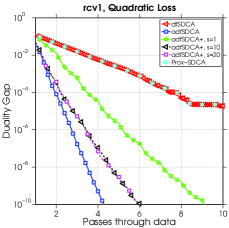
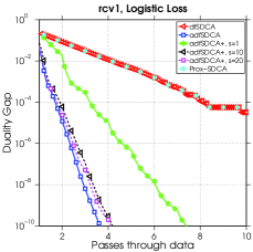
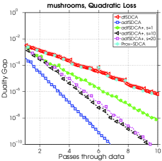
Figure 1: Comparing number of iterations among various algorithms.

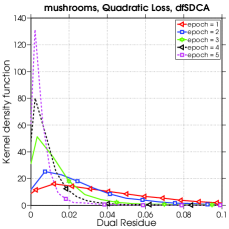
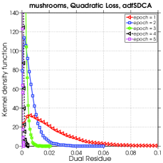
Figure 2: Comparing absolute value of dual residuals at each epoch between dfSDCA and adfSDCA.

References

- [1] Dominik Csiba, Zheng Qu, and Peter Richtárik. Stochastic dual coordinate ascent with adaptive probabilities. arXiv preprint arXiv:1502.08053, 2015.
- [2] Dominik Csiba and Peter Richtárik. Primal method for erm with flexible mini-batching schemes and non-convex losses. arXiv preprint arXiv:1506.02227, 2015.
- [3] Aaron Defazio, Francis Bach, and Simon Lacoste-Julien. Saga: A fast incremental gradient method with support for non-strongly convex composite objectives. In Advances in Neural Information Processing Systems, pages 1646–1654, 2014.
- [4] Cho-Jui Hsieh, Kai-Wei Chang, Chih-Jen Lin, S Sathiya Keerthi, and Sellamanickam Sundararajan. A dual coordinate descent method for large-scale linear svm. In Proceedings of the 25th international conference on Machine learning, pages 408–415. ACM, 2008.
- [5] Rie Johnson and Tong Zhang. Accelerating stochastic gradient descent using predictive variance reduction. In Advances in Neural Information Processing Systems, pages 315–323, 2013.
- [6] Jakub Konečný, Jie Liu, Peter Richtárik, and Martin Takáč. mS2GD: Mini-batch semi-stochastic gradient descent in the proximal setting. arXiv preprint arXiv:1410.4744, 2014.
- [7] Jakub Konečnỳ and Peter Richtárik. Semi-stochastic gradient descent methods. arXiv preprint arXiv:1312.1666, 2013.
- [8] Yu Nesterov. Efficiency of coordinate descent methods on huge-scale optimization problems. SIAM Journal on Optimization, 22(2):341–362, 2012.
- [9] Atsushi Nitanda. Stochastic proximal gradient descent with acceleration techniques. In Advances in Neural Information Processing Systems, pages 1574–1582, 2014.
- [10] Peter Richtárik and Martin Takáč. Iteration complexity of randomized block-coordinate descent methods for minimizing a composite function. Mathematical Programming, 144(1-2):1–38, 2014.
- [11] Peter Richtárik and Martin Takáč. On optimal probabilities in stochastic coordinate descent methods. Optimization Letters, pages 1–11, 2015.
- [12] Nicolas L Roux, Mark Schmidt, and Francis R Bach. A stochastic gradient method with an exponential convergence _rate for finite training sets. In Advances in Neural Information Processing Systems, pages 2663–2671, 2012.
- [13] Mark Schmidt, Reza Babanezhad, Mohamed Osama Ahmed, Aaron Defazio, Ann Clifton, and Anoop Sarkar. Non-uniform stochastic average gradient method for training conditional random fields. In International Conference on Artificial Intelligence and Statistics (AISTATS), 2015.
- [14] Mark Schmidt, Nicolas Le Roux, and Francis Bach. Minimizing finite sums with the stochastic average gradient. arXiv preprint arXiv:1309.2388, 2013.
- [15] Shai Shalev-Shwartz. SDCA without duality. arXiv preprint arXiv:1502.06177, 2015.
- [16] Shai Shalev-Shwartz, Yoram Singer, Nathan Srebro, and Andrew Cotter. Pegasos: Primal estimated sub-gradient solver for svm. Mathematical programming, 127(1):3–30, 2011.
- [17] Shai Shalev-Shwartz and Tong Zhang. Accelerated proximal stochastic dual coordinate ascent for regularized loss minimization. Mathematical Programming, pages 1–41, 2014.
- [18] Martin Takáč, Avleen Bijral, Peter Richtárik, and Nathan Srebro. Mini-batch primal and dual methods for SVMs. ICML 2013, 2013.
- [19] Martin Takáč, Peter Richtárik, and Nathan Srebro. Distributed mini-batch SDCA. arXiv preprint arXiv:1507.08322, 2015.
- [20] Rachael Tappenden, Martin Takáč, and Peter Richtárik. On the complexity of parallel coordinate descent. arXiv preprint arXiv:1503.03033, 2015.
- [21] Peilin Zhao and Tong Zhang. Stochastic optimization with importance sampling. arXiv preprint arXiv:1401.2753, 2014.