High order Nyström methods for transmission problems for Helmholtz equation

Abstract

We present superalgebraic compatible Nyström discretizations for the four Helmholtz boundary operators of Calderón’s calculus on smooth closed curves in 2D. These discretizations are based on appropriate splitting of the kernels combined with very accurate product-quadrature rules for the different singularities that such kernels present. A Fourier based analysis shows that the four discrete operators converge to the continuous ones in appropriate Sobolev norms. This proves that Nyström discretizations of many popular integral equation formulations for Helmholtz equations are stable and convergent. The convergence is actually superalgebraic for smooth solutions.

1 Introduction

The design of robust discretizations of the boundary integral equations in 2D has been an active research topic in the last decades. The analysis of Galerkin discretizations of boundary integral equations is by now well understood in the case of smooth boundaries and boundary data. Indeed, their stability can be established based on the coercivity of the principal parts of the boundary integral operators featured in the integral formulations (a first result along these lines can be traced back to [12]), and compact perturbation analysis arguments. On the other hand, although Nyström/collocation methods are simpler to implement, their analysis is somewhat more complicated. Given that for 2D problems boundary integral operators can be thought of as periodic pseudodifferential operators, the analysis of discretization schemes for boundary integral equations relies on Fourier analysis. Galerkin as well as Nyström/collocation methods for periodic integral equations have been fully analyzed for many periodic integral equations and these techniques have been also used to derive new methods as qualocation schemes, cf. [13] and references therein.

Boundary integral formulations of Helmholtz equations in a certain domain rely on single and double layer acoustic potentials and their Dirichlet and Neumann traces on the boundary of that domain. These traces lead to the natural definition of four boundary integral operators which are referred to as the Helmholtz boundary integral operators of Calderon’s calculus. In this paper we focus on Nyström methods based on suitable quadrature rules for the discretization of the four Helmholtz boundary integral operators that feature in Calderon’s calculus. These provide a means of defining fully discrete versions of these operators which can be used easily to discretize complicate formulations involving rather complex compositions of different boundary operators. Moreover, these discretizations can be easily used in conjunction with iterative solvers based on Krylov subspace methods.

The aim of this paper is not to propose new discretizations of the Helmholtz boundary integral operators. Actually, most of those considered here can be found and have been thoroughly analyzed in the literature, mostly by Kress (cf [6, 7] and references therein). Our objective is therefore different: we want to propose compatible discretizations of the four Helmholtz boundary integral operators that lead to superalgebraic schemes for most of the boundary integral formulations of the Helmholtz equation in 2D.

Helmholtz transmission problems for smooth interfaces provide a sufficiently complex environment for testing our discretizations as they feature all of the four Helmholtz boundary integral operators in Calderon’s calculus. Discretizations of integral formulations of other types of boundary conditions can be readily produced and analyzed with the methods we present in this paper.

Some of the formulations considered in this paper are direct, i.e. the unknowns are physical quantities of the problem (typically the trace and the normal derivative of the solution), others are indirect. Some of the indirect formulations considered in this text could be more economical from a computational point of view. Besides, some more sophisticated integral formulations lead to matrices with clustered eigenvalues, which usually ensures a faster convergence of Krylov methods such as GMRES. Demanding better spectral properties requires working with more complex formulations whose discretization could seem challenging at first sight. We will show that the discrete boundary layer operators can be used as black boxes in such a way that the discretization of any integral formulation, however complicated, is in fact straightforward. Moreover, for smooth data, we prove that the numerical solutions converge superalgebraically, that is, faster than any negative power of $N$, the number of degrees of freedom.

The paper is structured as follows: in Section 2 we discuss briefly the Helmholtz transmission problem and introduce the boundary layer potentials and operators for the Helmholtz equation. In Section 3 we reformulate these mappings as integral operators acting on spaces of $2\pi-$periodic functions via a parameterization of the interface. We present also their numerical discretizations and analyze their convergence. We next introduce compatible discretizations of the operators and derive convergence estimates in Sobolev setting. We conclude by showing in Section 4 how these compatible discretizations can be applied to solve numerically several boundary integral formulations of the original Helmholtz transmission problem. Well-posedness and convergence estimates are derived for the integral equations considered in this paper. Some numerical experiments are presented in the final Section 5.

2 Helmholtz transmission problems and boundary integral operators

We start introducing the domain of the transmission problem (see Figure 1). Let $D^{-}$ be a compact domain with smooth boundary $\Gamma$ which for simplicity we will assume to be simply connected. Denote also $D^{+}:=\mathbb{R}^{2}\setminus\overline{D^{-}}$. We will write $\gamma$ for the trace operator and $\partial_{n}$ for the unit normal derivative on $\Gamma$ pointing toward $D^{+}$. Given two wavenumbers $k_{+},k_{-}$ that are complex numbers with non-negative imaginary part, we consider the following Helmholtz transmission problem:

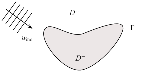
Figure 1: Sketch of the domain of the transmission problem

$$\begin{array}[]{rcl}\displaystyle\Delta u^{\rm+}+k_{+}^{2}u^{\rm+}\!\!\!&=&\!\!\!0\qquad\mathrm{in}\ D^{+}\\ \displaystyle\Delta u^{-}+k_{-}^{2}u^{-}\!\!\!&=&\!\!\!0\qquad\mathrm{in}\ D^{-}\\ \displaystyle{\gamma}u^{\rm+}\!-{\gamma}u^{-}\!\!\!&=&\!\!\!-{u}_{\rm inc},\ \displaystyle{\partial_{n}}u^{\rm+}\!-\!\displaystyle{\nu}{{\partial_{n}}}u^{-}=-\partial_{n}u_{\rm inc}\\ \displaystyle\partial_{r}u^{+}\!-\!{\rm i}k_{+}u^{+}\!\!\!&=&\!\!\!o(|{\bf r}|^{-1/2}).\end{array}$$ (1)

Here $\partial_{r}$ is the partial derivative on the radial direction and $u_{\rm inc}$ is an incident wave that is a solution of the Helmholtz problem for $k_{+}$ on a neighborhood of $\overline{D^{-}}$. We assume that the transmission problem above together with its adjoint, that is the transmission problem defined by taking $k_{\pm}$ in $D^{\mp}$, are uniquely solvable. For instance, if $k_{\pm}$ are real and $\nu>0$ these hypotheses are known to be satisfied. We refer to [4] for more comprehensive sets of values of $k_{\pm}$ and $\nu$ fulfilling these hypotheses.

Let

$$\Phi_{k}({\bf x}):=\frac{\rm i}{4}H_{0}^{(1)}(k|{\bf x}|)$$

($H_{0}^{(1)}$ is the Hankel function of first kind and order 0) be the outgoing fundamental solution of the Helmholtz equation in $\mathbb{R}^{2}$. The single and double layer operators are defined as follows

$${SL}_{k}\varphi:=\int_{\Gamma}\Phi_{k}(\>\cdot\>-\mathbf{y})\varphi(\mathbf{y}){\rm d}\sigma(\mathbf{y}),\qquad{DL}_{k}g:=\int_{\Gamma}\frac{\partial\Phi_{k}(\>\cdot\>-\mathbf{y})}{\partial\mathbf{n}(\mathbf{y})}g(\mathbf{y}){\rm d}\sigma(\mathbf{y}).$$ (2)

We stress that for any density, the layer operators define solutions of the Helmholtz equation in $\mathbb{R}^{2}\setminus\Gamma$ which satisfy, in addition, the radiation condition at infinity (last condition in (1)). Moreover, the third Green formula states

$$u^{\pm}=\mp\>{SL}_{k_{\pm}}\partial_{n}u_{\pm}\>\>\pm\>\>{DL}_{k_{\pm}}\>\gamma u_{\pm}.$$ (3)

Let us denote by $\gamma^{\pm},\partial_{n}^{\pm}$ the trace and respectively the normal derivative taken from $D^{\pm}$. We have then the jump properties

$$\gamma^{\pm}{SL}_{k} =V_{k} \partial_{n}^{\pm}{SL}_{k} =\mp\tfrac{1}{2}I+K^{\top}_{k}$$ (4)

$$\gamma^{\pm}{DL}_{k} =\pm\tfrac{1}{2}I+K^{\top}_{k} \partial_{n}^{\pm}{DL}_{k} =H_{k}$$

where $I$ denotes the identity, $V_{k}$ is the single layer operator, $K_{k}$ and $K_{k}^{\top}$ are the double layer and adjoint double layer operator, and $H_{k}$ is the hypersingular operator.

We can now proceed as follows: (a) we can use (4) and the transmission conditions stated in (1) to compute the Cauchy data of the solution $(u^{\pm},\partial_{n}^{\pm}u)$ and reconstruct these functions using (3); (b) we can try to write the $u^{\pm}$ in terms of some unknown densities associated with the potentials (2) and solve for these densities via equations obtained from (4). Approach (a) leads to the so-called direct methods whereas schemes obtained from (b) are known as indirect methods.

3 Associated periodic integral operators and their approximation

3.1 Periodic integral operators

Let us consider a smooth regular $2\pi-$periodic parameterization of the curve $\Gamma$ given by ${\bf x}:\mathbb{R}\to\Gamma$. First we set the transmission data

$$h(s):=-\big{(}\gamma_{\Gamma}u_{\rm inc}\circ{\bf x}\big{)}(s),\quad\eta(s):=-\big{(}\partial_{n}u_{\rm inc}\circ{\bf x}\big{)}(s)\,|{\bf x}^{\prime}(s)|.$$ (5)

We follow the same rule to reformulate layer potentials and boundary integral operators as $2\pi-$periodic integral operators in the following sense: for ${SL}_{k}$ and the associated boundary integral operators $V_{k}$ and $K_{k}^{\top}$, the norm of the parameterization $|{\bf x}^{\prime}(t)|$ ($t$ is the integration variable) is incorporated in the density function $\varphi$ in (2), whereas for ${DL}_{k}$, and the corresponding boundary integral operators $K_{k}$ and $H_{k}$ this term is incorporated in the kernels of these operators. In addition, the operators $K_{k}^{\top}$ and $H_{k}$ are multiplied by $|{\bf x}(s)|$, where $s$ will be used henceforth as the variable corresponding to the target point in all of the integral operators considered in this text. With these conventions, we write the single, double and adjoint double layer operator as follows

$${[}{\rm V}_{k}\varphi{]}(s) = \int_{0}^{2\pi}A(s,t)\log\sin^{2}\tfrac{s-t}{2}\varphi(t){\rm d}t+\int_{0}^{2\pi}B(s,t)\varphi(t){\rm d}t$$ (6)

$${[}{\rm K}_{k}g{]}(s) = \int_{0}^{2\pi}C(s,t)\sin^{2}\tfrac{s-t}{2}\log\sin^{2}\tfrac{s-t}{2}g(t){\rm d}t+\int_{0}^{2\pi}D(s,t)g(t){\rm d}t$$ (7)

$${[}{\rm K}^{\top}_{k}\varphi{]}(s) = \int_{0}^{2\pi}C(t,s)\sin^{2}\tfrac{t-s}{2}\log\sin^{2}\tfrac{t-s}{2}\varphi(t){\rm d}t+\int_{0}^{2\pi}D(t,s)\varphi(t){\rm d}t.$$ (8)

with

$$A(s,t) = -\frac{1}{4\pi}J_{0}(k|{\bf x}(s)-{\bf x}(t)|)$$

$$C(s,t) = -\frac{k({\bf x}(s)-{\bf x}(t))\cdot({x}_{2}^{\prime}(t),-{x_{1}^{\prime}(t)})}{|{\bf x}(s)-{\bf x}(t)|^{2}}\frac{J_{1}(k|{\bf x}(s)-{\bf x}(t)|)}{|{\bf x}(s)-{\bf x}(t)|}\>\frac{|{\bf x}(s)-{\bf x}(t)|^{2}}{\sin^{2}\tfrac{s-t}{2}}$$

$$B(s,t) = \frac{{\rm i}}{4}H_{0}^{1}(k|{\bf x}(s)-{\bf x}(t)|)-A(s,t)\log\sin^{2}\tfrac{s-t}{2}$$

$$D(s,t) = \frac{{\rm i}k}{4}H_{1}^{1}(k|{\bf x}(s)-{\bf x}(t)|)\frac{({\bf x}(s)-{\bf x}(t))\cdot({x}_{2}^{\prime}(t),-{x_{1}^{\prime}(t)})}{|{\bf x}(s)-{\bf x}(t)|}$$

$$-C(s,t)\sin^{2}\tfrac{s-t}{2}\log\sin^{2}\tfrac{s-t}{2}.$$

(Observe that ${\rm K}_{k}$ and ${\rm K}_{k}^{\top}$ are transpose to each other). Very well known properties of the Bessel functions imply that the functions $A,B,C,D$ are smooth functions if so is the map ${\bf x}$, as we have already assumed above.

Regarding the parameterized version of the hypersingular operator, the integration-by-parts like formula due to Maue [9] (see also [11]) allows to write ${\rm H}_{k}$ as the integro-differential operator

$$\left[{\rm H}_{k}g\right](s)=\left[{\rm D}{\sf V}_{k}{\rm D}\,g\right](s)-{\rm i}k^{2}\left[{\sf V}_{k}(({\bf x}^{\prime}(s)\cdot{\bf x}^{\prime}(\cdot))g\right](s).$$ (9)

Here, ${\rm D}\varphi:=\varphi^{\prime}$ is simply the differentiation operator.

3.2 Nyström Discretization

The structure of the kernels introduced in the previous section leads to tackle, apart from the derivative operator, the evaluation of integrals as

$$\left[\Psi\varphi\right](s):=\int_{0}^{2\pi}\psi(s-t)a(s,t)\varphi(t)\,{\rm d}t,$$ (10)

where $a$, $\psi$ are $2\pi-$periodic, with $a$ being smooth and $\psi$, in principle, singular at $0$. The operators defined in equation (10) are $2\pi-$periodic pseudodifferential operators (cf. [13, Ch.7]).

3.2.1 Trigonometric interpolation

Let us denote

$$\mathbb{T}_{N}:={\rm span}\>\langle e_{n}\>:\>-N<n\leq N\rangle,\quad\text{with}\quad e_{n}(t):=\exp({\rm i}nt),\quad(n\in\mathbb{Z})$$

the space of trigonometric polynomials of degree $N$. On $\mathbb{T}_{N}$ we consider the trigonometric interpolation problem on the uniform grid $\{j\pi/N\}$:

$$\mathbb{T}_{N}\ni P_{N}g\quad\text{s.t.}\quad(P_{N}g)(\tfrac{j\pi}{N})=g(\tfrac{j\pi}{N}),\ j=0,\ldots,2N-1,$$

The solution of the interpolating problem is given by

$$\sum_{n=-N+1}^{N}\left[\frac{1}{2N}\sum_{m=-N+1}^{N}g(\tfrac{j\pi}{N})e_{n}(-\tfrac{{\rm i}m\pi}{N})\right]e_{n}({\rm i}nt)$$ (11)

which can be computed in ${\cal O}(n\log n)$ operations using FFT.

3.2.2 Discrete operators

We now introduce

$$\left[\Psi_{N}\varphi\right](s):=\int_{0}^{2\pi}\psi(s-t)P_{N}\left[a(s,\cdot)\varphi\right](t)\,{\rm d}t\approx\left[\Psi\varphi\right](s)$$ (12)

as discrete approximations of (10). Clearly $\Psi_{N}\varphi$ depends only on the pointwise values of the density at the grid points, which justifies the use of the term “discrete” when referring to these operators.

Obviously, we are just working with a product-integration rule and the applicability of such procedure relies on being able to compute

$$\widehat{\psi}(n):=\frac{1}{2\pi}\int_{0}^{2\pi}\psi(t)e_{-n}(t)\,{\rm d}t,\quad n\in\mathbb{Z}$$

i.e. the Fourier coefficients of the weight function $\psi$. Fortunately, for the weight functions featured above, these Fourier coefficients can be computed explicitly. Indeed, for $\psi_{1}:=\log\sin^{2}\tfrac{t}{2}$ we have

$$\widehat{\psi}_{1}(n) = \tfrac{1}{2\pi}\int_{0}^{2\pi}\!\log(\sin^{2}\tfrac{t}{2})\>e_{-n}(t){\rm d}t=\tfrac{1}{2\pi}\int_{0}^{2\pi}\!\log(\sin^{2}\tfrac{t}{2})\>\cos(nt){\rm d}t$$

$$= \begin{cases}-2\log 4,&n=0,\\ -2|n|^{-1},&\text{otherwise},\end{cases}$$

whereas for $\psi_{2}:=\sin^{2}\tfrac{t}{2}\log\sin^{2}\tfrac{t}{2}$ straightforward calculations yield

$$\widehat{\psi}_{2}(n) = \tfrac{1}{2\pi}\int_{0}^{2\pi}\!\sin^{2}\tfrac{t}{2}\log(\sin^{2}\tfrac{t}{2})\>e_{-n}(t){\rm d}t$$

$$= \tfrac{1}{8\pi}\int_{0}^{2\pi}\log(\sin^{2}\tfrac{t}{2})\>\left(2\cos(nt)-\cos(n-1)t-\cos(n+1)t\right){\rm d}t$$

$$= \begin{cases}\tfrac{1}{2},&n=0,\\ -\tfrac{3}{8},&|n|=1,\\ \tfrac{1}{4}\big{[}\tfrac{1}{|n+1|}+\tfrac{1}{|n-1|}-\tfrac{2}{|n|}\big{]},&\text{otherwise}.\end{cases}$$

We stress that the calculation in the case of the weight $\psi_{1}$ can be traced back to [8, 10] (see also [7]). For the remaining case, $\psi_{0}\equiv 1$, the same approach gives us (see (11))

$$\int_{0}^{2\pi}(P_{N}g)(t)\,{\rm d}t = \sum_{n=-N+1}^{N}\left[\frac{1}{2N}\sum_{m=-N+1}^{N}g(\tfrac{j\pi}{N})\exp(-\tfrac{{\rm i}mn\pi}{N})\right]\int_{0}^{2\pi}\exp(int)\,{\rm d}t$$

$$= \frac{\pi}{N}\sum_{j=0}^{2N-1}g\big{(}\tfrac{j\pi}{N}\big{)},$$

i.e., the trapezoidal rule. Therefore, for $\psi\equiv 1$, we simply have

$$\left[\Psi_{N}\varphi\right](s)=\frac{\pi}{N}\sum_{j=0}^{2N-1}a\big{(}s,\tfrac{j\pi}{N}\big{)}\varphi(\tfrac{j\pi}{N}\big{)}.$$

3.2.3 Discrete Helmholtz Boundary Integral Operators

For the single layer operator we work with two types of discretizations. The first one, proposed originally by Kress (cf. [7] and references therein) is simply

$${[}{\rm V}_{k,N}\varphi{]}(s) := \int_{0}^{2\pi}\psi_{1}(s-t)\left[P_{N}A(s,\cdot)\varphi\right](t)\,{\rm d}t+\int_{0}^{2\pi}[P_{N}B(s,\cdot)\varphi](t){\rm d}t.$$ (13)

One can use the same approach for the double layer operator and obtain

$${[}{\rm K}_{k,N}\varphi{]}(s):=\!\int_{0}^{2\pi}\!\!\psi_{1}(s-t)[P_{N}C(s,\cdot)\sin^{2}\tfrac{s-\cdot}{2}\>\varphi](t){\rm d}t+\!\int_{0}^{2\pi}\left[P_{N}D(s,\cdot)\varphi\right](t){\rm d}t.$$ (14)

The operator ${\rm K}_{k,N}^{\top}$ can be defined accordingly.

Alternatively, we can proceed in a different way and define the more accurate approximation

$${[}\widetilde{\rm K}_{k,N}g{]}(s) := \int_{0}^{2\pi}\!\!\psi_{2}(s-t)P_{N}[C(s,\cdot)g](t)\,{\rm d}t+\int_{0}^{2\pi}[P_{N}D(s,\cdot)g](t){\rm d}t.$$ (15)

The operator $\widetilde{{\rm K}}^{\top}_{k,N}$ can be obviously defined in the same manner.

We can actually use the same approach for the single layer operator ${\rm V}_{k}$. Indeed, let us write first

$$A(s,t) = -\frac{1}{4\pi}+\frac{1-J_{0}(k|{\bf x}(s)-{\bf x}(t)|)}{4\pi\sin^{2}\tfrac{s-t}{2}}\sin^{2}\tfrac{s-t}{2}=:-\frac{1}{4\pi}+\widetilde{A}(s,t)\sin^{2}\tfrac{s-t}{2}.$$ (16)

We point out that function $A(s,t)$ is smooth with

$$\widetilde{A}(s,s)\equiv\frac{k^{2}}{4\pi}|{\bf x}^{\prime}(s)|.$$

Hence, using the Bessel operator defined as

$$\left[\Lambda\varphi\right](s):=-\frac{1}{4\pi}\int_{0}^{2\pi}\log\sin^{2}\tfrac{s-t}{2}\>\varphi(t)\,{\rm d}t,$$

we have derived the following alternative expression for the single layer operator

$${\rm V}_{k}\varphi = \Lambda\varphi+\int_{0}^{2\pi}\widetilde{A}(\>\cdot\>,t)\psi_{2}(\>\cdot\>-t)\varphi(t)\,{\rm d}t+\int_{0}^{2\pi}B(\>\cdot\>,t)\varphi(t)\,{\rm d}t=:\Lambda\varphi+{\rm R}_{k}\varphi,$$

which can be exploited to lead to the following approximation

$$\big{[}\widetilde{\rm V}_{k,N}\varphi\big{]}(s) := \big{[}\Lambda\varphi\big{]}(s)+\int_{0}^{2\pi}\psi_{2}(s-t)\>P_{N}[\widetilde{A}(s,\cdot)\varphi](t)\,{\rm d}t+\int_{0}^{2\pi}P_{N}[\widetilde{B}(s,\cdot)\varphi](t)\,{\rm d}t$$ (17)

$$=: \big{[}\Lambda\varphi\big{]}(s)+\big{[}\widetilde{\rm R}_{k,N}\varphi\big{]}(s).$$

Obviously, $\widetilde{\rm V}_{k,N}$ can be applied, in principle, only to trigonometric polynomials, since otherwise the first term gives rise to an infinite series. As we will see later, this is not a severe constraint for the numerical approximations we propose.

Finally, applying integration by parts and making use of the same quadrature rules, we have

$${\rm H}_{k} = {\rm D}\Lambda{\rm D}+{\rm T}_{k}$$ (18)

with

$$\big{[}{\rm T}_{k}\varphi\big{]}(s)=\int_{0}^{2\pi}E(s,t)\log\sin^{2}\tfrac{s-t}{2}\varphi(t)\>{\rm d}t+\int_{0}^{2\pi}F(s,t)\varphi(t)\>{\rm d}t$$

where

$$E(s,t) := -\partial_{s}\partial_{t}\widetilde{A}(s,t)\sin^{2}\tfrac{s-t}{2}+\tfrac{1}{2}\big{(}\partial_{s}\widetilde{A}(s,t)-\partial_{t}\widetilde{A}(s,t)\big{)}\sin(s-t)$$

$$+\tfrac{1}{2}\widetilde{A}(s,t)\cos(s-t)-{\rm i}k^{2}\big{(}{\bf x}^{\prime}(s)\cdot{\bf x}^{\prime}(t)\big{)}A(s,t)$$

$$F(s,t) := -\partial_{s}\partial_{t}{B}(s,t)+\tfrac{1}{2}\big{(}\partial_{s}\widetilde{A}(s,t)-\partial_{t}\widetilde{A}(s,t)\big{)}\sin(s-t)$$

$$+\widetilde{A}(s,t)(\tfrac{1}{2}+\cos(s-t))-{\rm i}k^{2}({\bf x}^{\prime}(s)\cdot{\bf x}^{\prime}(t))B(s,t).$$

Then, following the same convention, we can define

$${\rm H}_{k,N}\varphi:={\rm D}\Lambda{\rm D}\varphi+{\rm T}_{k,N}\varphi$$ (19)

with

$$\big{[}{\rm T}_{k,N}\varphi\big{]}(s)=\int_{0}^{2\pi}\psi_{1}(s-t)\left[P_{N}E(s,\cdot)\varphi\right](t){\rm d}t+\int_{0}^{2\pi}[P_{N}F(s,\cdot)\varphi](t){\rm d}t\\$$

Again ${\rm H}_{k,N}$ is not a full discrete operators, but when applied to trigonometric polynomials it can be computed exactly which turns out to be enough for our purposes.

3.3 Convergence analysis

We develop our analysis in periodic Sobolev norms. For any $p\in\mathbb{R}$ we first define the Sobolev norm

$$\|\varphi\|^{2}_{p}:=|\widehat{\varphi}(0)|^{2}+\sum_{n\neq 0}|n|^{2p}|\widehat{\varphi}(n)|^{2}.$$

The periodic Sobolev spaces of order $p$, denoted in what follows by $H^{p}$, can be defined, for instance, as the completion of trigonometric polynomials in this norm.

We are ready to state the main theorem. The proof follows from application of similar ideas to those introduced in [7, Ch. 12 and 13] (see also [1]). Let us point out that henceforth, for given $A:X\to Y$, we denote by $\|A\|_{X\to Y}$ its operator norm.

Theorem 3.1.

Let $p>1/2$ and $q\geq-1$ with $p+q>1/2$. Then, if ${\rm A}\in\{{\rm K}_{k},{\rm K}_{k}^{\top},{\rm V}_{k},{\rm H}_{k}\}$ and ${\rm A}_{N}$ is the corresponding approximation, i.e., ${\rm A}_{N}\in\{{\rm K}_{k,N},{\rm K}_{k,N}^{\top},{\rm V}_{k,N},{\rm H}_{k,N}\}$,

$$\|{\rm A}-{\rm A}_{N}\|_{H^{p+q}\to H^{p}} \leq C_{p,q}N^{-q-\min\{p,1\}}.$$ (20)

On the other hand, for ${\rm A}\in\{{\rm K}_{k},{\rm K}_{k}^{\top},{\rm V}_{k}\}$ and $\widetilde{\rm A}_{N}\in\{\widetilde{\rm K}_{k,N},\widetilde{\rm K}_{k,N}^{\top},\widetilde{\rm V}_{k,N}\}$ the corresponding discretization, we have for $q\geq-3$ with $p+q>1/2$.

$$\|{\rm A}-\widetilde{\rm A}_{N}\|_{H^{p+q}\to H^{p}}\!\! \leq \!\!C_{p,q}N^{-q-\min\{p,3\}}.$$ (21)

Proof For any function $\psi$ we denote the convolution operator in the usual manner:

$$[\psi*\varphi](s):=\int_{0}^{2\pi}\psi(s-t)\varphi(t)\,{\rm d}t={\sum_{n=-\infty}^{\infty}\widehat{\psi}(n)\widehat{\varphi}(n)e_{n}(s)}.$$

Then it is straightforward to check that for $\varphi$ smooth enough, see (10),

$$[\Psi\varphi](s) = \int_{0}^{2\pi}a(s,t)\psi(s-t)\varphi(t)\,{\rm d}t=\sum_{n=-\infty}^{\infty}a_{n}(s)[\psi*(e_{n}\varphi)](s)$$

where $e_{n}(s)=\exp({\rm i}ns)$ and

$$a_{n}(s):=\frac{1}{2\pi}\int_{0}^{2\pi}a(s,t)e_{-n}(t){\rm d}t$$

is the $n$th Fourier coefficient of $a(s,\cdot)$. Since function $a$ is assumed to be smooth, then for any $P$ it holds that

$$\sup_{n\in\mathbb{N}}(1+|n|)^{P}\|a_{n}\|_{L^{\infty}(0,2\pi)}<C_{P}.$$

Let us restrict ourselves to the cases $\psi=\psi_{m}$, for $m=0,1,2$ (see the beginning of subsection 3.2.2). Denote then by $\Psi_{m}$ the corresponding operator and by $\Psi_{m,N}$, its numerical approximation cf. (12). Clearly, the proof of this Theorem can be reduced to studying

$$(\Psi_{m}-\Psi_{m,N})\varphi=\sum_{n=-\infty}^{\infty}a_{n}\psi_{m}*(e_{n}\varphi-P_{N}(e_{n}\varphi)).$$

We will make use of the following results:

• for $m=1,2$ it holds

  $$\|\psi_{m}*\varphi\|_{p}\leq C_{q}\|\varphi\|_{p-q},\quad q\leq 2m-1$$

  whereas for $m=0$

  $$\|\psi_{0}*\varphi\|_{p}=2\pi|\widehat{\varphi}(0)|\leq 2\pi\|\varphi\|_{p+q},\quad\forall q\in\mathbb{R};$$

  Indeed, for $m=1,2$

  $$|\widehat{\psi}_{m}(n)|\leq C_{m}(1+|n|)^{1-2m}$$

  with $C_{m}$ independent of $m$ which implies

  $$\|\psi_{m}*\varphi\|_{p}^{2} = |\widehat{\psi}_{m}(0)\widehat{\varphi}(0)|^{2}+\sum_{n=-\infty}^{\infty}|n|^{2p}|\widehat{\psi}(n)\widehat{\varphi}(n)|^{2}$$

  $$\leq C^{2}_{m}\left[|\widehat{\psi}_{m}(0)\widehat{\varphi}(0)|^{2}+\sum_{n=-\infty}^{\infty}|n|^{2(p+1-2m)}|\widehat{\varphi}(n)|^{2}\right]=C^{2}_{m}\|\varphi\|^{2}_{p-2m+1};$$

• the convergence estimate for the trigonometric interpolant [13, Theorem 8.2.1]

  $$\|P_{N}\varphi-\varphi\|_{p}\leq C_{p,q}N^{-q}\|\varphi\|_{p+q},\quad\forall p,q\geq 0,\quad p+q>1/2;$$ (22)

• the fact that $H^{p}$ for $p>1/2$ is an algebra, cf [13, Lemma 5.13.1] and therefore

  $$\|a\varphi\|_{p}\leq C_{p}\|a\|_{p}\|\varphi\|_{p};$$

• the obvious bound $\|e_{n}\|_{p}\leq\max\{1,|n|^{p}$}.

We are ready to analyze the approximation error of the discrete operators. First, for $m=0$, that is, for integral operators with smooth kernel, we have

$$\|(\Psi_{0}-\Psi_{0,N})\varphi\|_{p} \leq C\!\sum_{n=-\infty}^{\infty}\!\|a_{n}\|_{p}\|\psi_{0}*(e_{n}\varphi-P_{N}(e_{n}\varphi))\|_{p}$$

$$= 2\pi C_{p}\sum_{n=-\infty}^{\infty}\|a_{n}\|_{p}\|e_{n}\varphi-P_{N}(e_{n}\varphi)\|_{0}$$

$$\leq C_{p,q}N^{-p-q}\sum_{n=-\infty}^{\infty}\|a_{n}\|_{p}\|e_{n}\|_{p+q}\|\varphi\|_{p+q}$$

$$\leq C_{p,q}N^{-p-q}\bigg{[}\sum_{n=-\infty}^{\infty}\|a_{n}\|_{p}(1+|n|)^{p+q}\bigg{]}\|\varphi\|_{p+q}$$

$$\leq C_{p,q}^{\prime}N^{-p-q}\|\varphi\|_{p+q}$$

for all $p+q\geq 1$.

Let us examine the case $m=2$. If $p\geq 3$, we can proceed similarly to conclude

$$\|(\Psi_{2}-\Psi_{2,N})\varphi\|_{p} \leq \sum_{n=-\infty}^{\infty}\|a_{n}\|_{p}\|e_{n}\varphi-P_{N}(e_{n}\varphi)\|_{p-3}$$

$$\leq C_{p,q}N^{-q-3}\sum_{n=-\infty}^{\infty}\|a_{n}\|_{p}\|e_{n}\|_{{p+q}}\|\varphi\|_{p+q}\leq C_{p,q}N^{-q-3}\|\varphi\|_{p+q},$$

provided that $p+q>1/2$ and $q\geq-3$. If $p\in[0,3]$, we can only get convergence estimates for the interpolator in $H^{0}$ (we can not expect faster convergence in weaker norms). Therefore we have instead

$$\|(\Psi_{2}-\Psi_{2,N})\varphi\|_{p} \leq \sum_{n=-\infty}^{\infty}\|a_{n}\|_{p}\|e_{n}\varphi-P_{N}(e_{n}\varphi)\|_{0}\leq C_{p,q}N^{-p-q}\|\varphi\|_{p+q}.$$

Collecting these bounds, the result for $m=3$ follows readily.

Case $m=1$ is left as exercise for the reader. $\Box$

We recall the functional properties of the boundary operators in the Sobolev setting. Define

$${\cal D}_{k}:=\begin{bmatrix}-{\rm K}_{k}&{\rm V}_{k}\\ -{\rm H}_{k}&{\rm K}^{\top}_{k}\end{bmatrix}.$$

Then, ${\cal D}_{k}:H^{p+1}\times H^{p}\to H^{p+1}\times H^{p}$ is continuous for any $p\in\mathbb{R}$. Actually it holds

$${\rm K}_{k},{\rm K}_{k}^{\top},{\rm R}_{k}:H^{p}\to H^{p+3}.$$ (23)

This extra regularizing property has been repeatedly used in the design and analysis of boundary integral methods for Helmholtz equation.

If we define

$${\cal D}_{k,N}:=\begin{bmatrix}-{\rm K}_{k,N}&{\rm V}_{k,N}\\[4.73611pt] -{\rm H}_{k,N}&{\rm K}^{\top}_{k,N}\end{bmatrix},\quad\widetilde{\cal D}_{k,N}:=\begin{bmatrix}-\widetilde{\rm K}_{k,N}&{\rm\widetilde{V}}_{k,N}\\[4.73611pt] -{\rm H}_{k,N}&\widetilde{\rm K}^{\top}_{k,N}\end{bmatrix},\quad$$

the following result can be easily derived from Theorem 3.1

Proposition 3.1.1.

For any $p>1/2$,

$${\cal D}_{k,N},\widetilde{\cal D}_{k,N}:H^{p+1}\times H^{p}\to H^{p+1}\times H^{p}$$ (24)

are uniformly continuous. Moreover, if $p>1/2$ and $q\geq-1$ with $p+q>1/2$,

$$\|{\cal D}_{k,N}-{\cal D}_{k}\|_{H^{p+q}\times H^{p+q}\to H^{p}\times H^{p}}+\|\widetilde{\cal D}_{k,N}-{\cal D}_{k}\|_{H^{p+q}\times H^{p+q}\to H^{p}\times H^{p}}\leq CN^{-q-\min\{1,p\}},$$ (25)

and, for $q\geq-2$, $p>1/2$ and $p+q>1/2$,

$$\|\widetilde{\cal D}_{k,N}-{\cal D}_{k}\|_{H^{p+q+1}\times H^{p+q}\to H^{p+1}\times H^{p}}\leq C{N^{-q-\min\{2,p\}}}.$$ (26)

Proof.

Define

$${\cal E}_{k}:=\begin{bmatrix}-{\rm K}_{k}&{\rm V}_{k}\\ -{\rm T}_{k}&{\rm K}^{\top}_{k}\end{bmatrix},\quad{\cal E}_{k,N}:=\begin{bmatrix}-{\rm K}_{k,N}&{\rm V}_{k,N}\\ -{\rm T}_{k,N}&{\rm K}^{\top}_{k,N}\end{bmatrix}.$$ (27)

Then

$${\cal D}_{k,N}-{\cal D}_{k}={\cal E}_{k,N}-{\cal E}_{k}.$$ (28)

Equation (20) in Theorem 3.1 proves (25) since

$$\|{\rm K}_{k,N}-{\rm K}_{k}\|_{H^{p+q}\to\times H^{p}} \leq CN^{-q-\min\{1,p\}}$$ (29a)

$$\|{\rm K}^{\top}_{k,N}-{\rm K}^{\top}_{k}\|_{H^{p+q}\to H^{p}} \leq CN^{-q-\min\{1,p\}}$$ (29b)

$$\|{\rm V}_{k,N}-{\rm V}_{k}\|_{H^{p+q}\to H^{p}} \leq CN^{-q-1-\min\{1,p\}}$$ (29c)

$$\|{\rm T}_{k,N}-{\rm T}_{k}\|_{H^{p+q}\to H^{p}} \leq CN^{-q-\min\{1,p\}}$$ (29d)

which hold for $p+q>1/2$ and $q\geq-1$. Moreover, from the mapping properties of the continuous operators, these estimates with $q=0$ imply the first result for ${\cal D}_{k,N}$.

For the second estimate, we start now from

$$\widetilde{\cal D}_{k,N}-{\cal D}_{k}=\widetilde{\cal F}_{k,N}-{\cal F}_{k}$$ (30)

where

$${\cal F}_{k}:=\begin{bmatrix}-{\rm K}_{k}&{\rm R}_{k}\\ -{\rm T}_{k}&{\rm K}^{\top}_{k}\end{bmatrix},\quad\widetilde{\cal F}_{k,N}:=\begin{bmatrix}-\widetilde{\rm K}_{k,N}&\widetilde{\rm R}_{k,N}\\ -{\rm T}_{k,N}&\widetilde{\rm K}^{\top}_{k,N}\end{bmatrix},$$ (31)

for which we have the error convergence estimates

$$\|\widetilde{\rm K}_{k,N}-{\rm K}_{k}\|_{H^{p^{\prime}+q^{\prime}}\to H^{p^{\prime}}} \leq CN^{-q^{\prime}-\min\{3,p^{\prime}\}},\quad q^{\prime}\geq-3$$ (32a)

$$\|\widetilde{\rm K}^{\top}_{k,N}-{\rm K}^{\top}_{k}\|_{H^{p^{\prime}+q^{\prime}}\to H^{p^{\prime}}} \leq CN^{-q^{\prime}-\min\{3,p^{\prime}\}},\quad q^{\prime}\geq-3$$ (32b)

$$\|\widetilde{\rm R}_{k,N}-{\rm R}_{k}\|_{H^{p^{\prime}+q^{\prime}}\to H^{p^{\prime}}} \leq CN^{-q^{\prime}-\min\{3,p^{\prime}\}},\quad q^{\prime}\geq-3$$ (32c)

$$\|{\rm T}_{k,N}-{\rm T}_{k}\|_{H^{p^{\prime}+q^{\prime}}\times H^{p^{\prime}}} \leq CN^{-q^{\prime}-\min\{1,p^{\prime}\}},\quad q^{\prime}\geq-1.$$ (32d)

(With the restriction $p^{\prime}+q^{\prime}>1/2$ in all these cases). Choosing $q^{\prime}=q$ and $p^{\prime}=p$ in all the estimates in (32) we get (25) which, in particular, implies (24) as a simple consequence. To prove (26), we take $(p^{\prime},q^{\prime})=(p+1,q)$ in (32a), $(p^{\prime},q^{\prime})=(p,q)$ in (32b), $(p^{\prime},q^{\prime})=(p+1,q-1)$ in (32c) and $(p^{\prime},q^{\prime})=(p,q+1)$ in (32d). ∎

In short, we have shown in this section two different types of discrete versions of the Helmholtz boundary layer operators. The first type of discretization is simpler and works well for equations stated in $H^{p}\times H^{p}$ such as the equations of the second kind where the hypersingular operator is not the leading term, either because it does not appear or because the strong singular part is canceled out. The second type of discretization involving the operators $\widetilde{\cal D}_{k,N}$ turns out to be more appropriate for formulations in the natural space $H^{p+1}\times H^{p}$ or for complex formulations where the operators are more involved and/or the operator ${\rm H}_{k}$ plays a dominant role. Actually, we could keep ${\rm K}_{k,N}$ and ${\rm K}^{\top}_{k,N}$ in $\widetilde{\cal D}_{k,N}$ and the desired convergence property, namely $\|\widetilde{\cal D}_{k,N}-{\cal D}_{k}\|_{H^{p}\times H^{p+1}\to H^{p}\times H^{p+1}}\to 0$ for any $p>1/2$, still holds. We have prefered, however, to collect in $\widetilde{\cal D}_{k,N}$ the more accurate discretization. We will consider several examples of these cases in next section.

4 Boundary integral equations for transmission problems and their Nyström discretizations

We consider numerical approximations of several well-posed formulations of the transmission problem (1) presented in Section 2. Equipped with the discrete operators introduced and analyzed in the previous section, the stability and convergence of the resulting schemes can be now easily proven.

For the sake of a simpler notation, we will denote in this section only by ${\rm V}_{\pm},$ ${\rm H}_{\pm},$ etc the corresponding layer operators for $k_{\pm}$. Their discrete versions will be denoted, as before, by simply adding the subscript $N$.

First we consider the Kress-Roach formulation cf [5]. Defining

$${\cal L}_{1}\!\begin{bmatrix}a\\ \varphi\end{bmatrix}:=\left(\!\tfrac{1+\nu}{2}{\cal I}\!+\!\begin{bmatrix}\nu{\rm K}_{-}-{\rm K}_{+}&{\rm V}_{+}-{\rm V}_{-}\\ \nu({\rm H}_{-}-{\rm H}_{+})&\nu{\rm K}^{\top}_{+}-{\rm K}^{\top}_{-}\\ \end{bmatrix}\!\right)\begin{bmatrix}a\\ \varphi\end{bmatrix},$$

where ${\cal I}$ is the identity operator matrix, this formulation amounts to solving the system of boundary equations

$${\cal L}_{1}\begin{bmatrix}a\\ \varphi\end{bmatrix}=\begin{bmatrix}f\\ \lambda\end{bmatrix}.$$ (33)

It is well known that if $(f,\lambda)=(h,\nu\,\eta)$ cf. (5), then the unique solution is $a=u_{\rm t}\circ{\bf x}$, $\varphi=|{\bf x}^{\prime}|(\partial_{n}u_{\rm t})\circ{\bf x}$ where $u_{t}$ is exterior part of the total wave: $u_{\rm t}=u_{+}+u_{\rm inc}$. Clearly, once this equation is solved, taking into account the transmission conditions (1), we can evaluate $u^{\pm}$ by means of (2).

The discrete versions of the operators $\mathcal{L}_{1}$ are given by

$${\cal L}_{1,N}\!\! := \!\tfrac{1+\nu}{2}{\cal I}+{\cal P}_{N}\begin{bmatrix}\nu{\rm K}_{-,N}-{\rm K}_{+,N}&{\rm V}_{+,N}-{\rm V}_{-,N}\\ \nu({\rm H}_{-,N}-{\rm H}_{+,N})&\nu{\rm K}^{\top}_{+,N}-{\rm K}^{\top}_{-,N}\end{bmatrix}\!$$

$$= \!\tfrac{1+\nu}{2}{\cal I}+{\cal P}_{N}\begin{bmatrix}\nu{\rm K}_{-,N}-{\rm K}_{+,N}&{\rm V}_{+,N}-{\rm V}_{-,N}\\ \nu({\rm T}_{-,N}-{\rm T}_{+,N})&\nu{\rm K}^{\top}_{+,N}-{\rm K}^{\top}_{-,N}\end{bmatrix}\!$$

(recall (18)-(19)) where

$${\cal P}_{N}=\begin{bmatrix}P_{N}\\ &P_{N}\end{bmatrix}.$$

Thus, the discrete problem is given by

$${\cal L}_{1,N}\begin{bmatrix}a_{N}\\ \varphi_{N}\end{bmatrix}=\begin{bmatrix}P_{N}f\\ P_{N}\lambda\end{bmatrix}$$ (34)

Observe that the last equation implies that $(a_{N},\varphi_{N})\in\mathbb{T}_{N}\times\mathbb{T}_{N}$ which allows us to reformulate the method as a true Nyström scheme, where the unknowns are the pointwise values of the densities at the grid points $\{\tfrac{j\pi}{N}\}$.

We will consider next the Costabel-Stephan formulation [2]: Let

$${\cal L}_{2} := \begin{bmatrix}-({\rm K}_{-}+{\rm K}_{+})&\nu^{-1}{\rm V}_{+}+{\rm V}_{-}\\ -({\rm H}_{-}+\nu{\rm H}_{+})&{\rm K}^{\top}_{+}+{\rm K}^{\top}_{-}\end{bmatrix}$$

$$= \!(1+\nu^{-1})\begin{bmatrix}&\Lambda\\ -\nu\mathrm{D\Lambda D}\end{bmatrix}+\begin{bmatrix}-{\rm K}_{-}-{\rm K}_{+}&{\nu}^{-1}\widetilde{\rm R}_{+}+\widetilde{\rm R}_{-}\\ -({\rm T}_{-}+\nu{\rm T}_{+})&{\rm K}^{\top}_{+}+{\rm K}^{\top}_{-}\end{bmatrix}$$

and the associated system of integral equations

$${\cal L}_{2}\begin{bmatrix}a\\ \varphi\end{bmatrix}=\begin{bmatrix}f\\ \lambda\end{bmatrix}.$$ (35)

In this case, if we take $(f,\lambda)=(h,\eta)$, then $(a,\varphi)=\left(u_{\rm t}\circ{\bf x},|{\bf x}^{\prime}|(\partial_{n}u_{\rm t})\circ{\bf x}\right)$ is again the exact solution.

Letting

$$\widetilde{\cal L}_{2,N}\!\! := \!(1+\nu^{-1})\begin{bmatrix}&\Lambda\\ -\nu\mathrm{D\Lambda D}\end{bmatrix}+{\cal P}_{N}\begin{bmatrix}-\widetilde{\rm K}_{-,N}-\widetilde{\rm K}_{+,N}&{\nu}^{-1}\widetilde{\rm R}_{+,N}+\widetilde{\rm R}_{-,N}\\ -({\rm T}_{-,N}+\nu{\rm T}_{+,N})&\widetilde{\rm K}^{\top}_{+,N}+\widetilde{\rm K}^{\top}_{-,N}\end{bmatrix},$$

the method we propose for solving (35) can be written in operational form as follows

$$\widetilde{\cal L}_{2,N}\begin{bmatrix}a_{N}\\ \varphi_{N}\end{bmatrix}=\begin{bmatrix}P_{N}f\\ P_{N}\lambda\end{bmatrix}.$$ (36)

As before, $(a_{N},\varphi_{N})\in\mathbb{T}_{N}\times\mathbb{T}_{N}$ for any pair $(f,\lambda)$ on the right hand side. (This can be easily seen by noticing that the leading part in $\widetilde{{\cal L}}_{2,N}$ is diagonal in the complex exponential bases).

The so-called regularized combined field integral equation, proposed in [3] will be also analyzed here. Let

$${\cal L}_{3}=\frac{1}{\nu+1}{\cal L}_{1}+\frac{2}{\nu+1}\begin{bmatrix}&{\rm V}_{\kappa}\\ -\nu{\rm H}_{\kappa}\end{bmatrix}{\cal L}_{2}=\begin{bmatrix}\frac{1}{2}I+{\rm K}_{-}&-\nu^{-1}{\rm V}_{-}\\ \nu{\rm H}_{-}&\frac{1}{2}I-{\rm K}_{-}^{\top}&\end{bmatrix}+{\mathcal{R}}_{\kappa}{\cal L}_{2}$$

with

$${\cal R}_{\kappa}:=\frac{1}{\nu+1}\begin{bmatrix}I&2{\rm V}_{\kappa}\\ -2\nu{\rm H}_{\kappa}&\nu I\end{bmatrix}.$$

The boundary integral equation is then given by

$${\cal L}_{3}\begin{bmatrix}a\\ \varphi\end{bmatrix}=\mathcal{R}_{\kappa}\begin{bmatrix}f\\ \lambda\end{bmatrix},\quad$$ (37)

It can be shown (see [3]) that this system of integral equations admits a unique solution provided that ${\kappa}$ is chosen to be a complex number with positive imaginary part. Moreover, this parameter can be adjusted to make eigenvalues cluster around $1$. Besides, by construction if we plug $(h,\eta)$ in the right hand side, the unique solution is $(u_{\rm t}\circ{\bf x},|{\bf x}^{\prime}|(\partial_{n}u_{\rm t})\circ{\bf x})$. In other words, this is a new direct method where ${\cal R}_{k}$ works as some sort of preconditioner for ${\cal L}_{2}$.

The discretization of the regularized equations is done as follows. First, we set

$${\mathcal{R}}_{\kappa,N}:=\frac{1}{\nu+1}\begin{bmatrix}I&2\Lambda+P_{N}\widetilde{\mathrm{R}}_{\kappa,N}\\ -2\nu\mathrm{D\Lambda D}-2\nu P_{N}\mathrm{T}_{\kappa,N}&\nu I\end{bmatrix}$$

and next we define

$$\widetilde{\cal L}_{3,N}\!\! := \!\!\!\!\begin{bmatrix}\frac{1}{2}I+P_{N}\widetilde{\rm K}_{-,N}&-\nu^{-1}\Lambda-\nu^{-1}P_{N}\widetilde{\rm R}_{-,N}\\ \nu\mathrm{D}\Lambda\mathrm{D}+\nu P_{N}{\rm T}_{-,N}&\frac{1}{2}I-P_{N}\widetilde{\rm K}_{-,N}^{\top}\end{bmatrix}+{\mathcal{R}}_{\kappa,N}\widetilde{\cal L}_{2,N}$$

$$= \begin{bmatrix}\frac{1}{2}I&-\nu^{-1}\Lambda\\ \nu\mathrm{D}\Lambda\mathrm{D}&\frac{1}{2}I\end{bmatrix}+{\cal P}_{N}\begin{bmatrix}\widetilde{\rm K}_{-,N}&\nu^{-1}\widetilde{\rm R}_{-,N}\\ \nu{\rm T}_{-,N}&-\widetilde{\rm K}_{-,N}^{\top}\end{bmatrix}+{\mathcal{R}}_{\kappa,N}\widetilde{\cal L}_{2,N}$$

(Observe that the first matrix operator maps $\mathbb{T}_{N}\times\mathbb{T}_{N}$ into itself.) The numerical algorithm, in operator form, is given by

$$\widetilde{\cal L}_{3,N}\begin{bmatrix}a_{N}\\ \varphi_{N}\end{bmatrix}={\cal R}_{\kappa,N}\begin{bmatrix}P_{N}f\\ P_{N}\lambda\end{bmatrix}.$$ (38)

Observe again that the right-hand-sides are trigonometric polynomials, and thus so are the solutions of these discrete problems .

We also investigate an integral formulation based on an indirect method. That is, unlike the formulations considered so far, the unknown is not immediately related to traces on the boundary of the solution of the transmission problem. This integral formulation, has an interesting feature: the solution of the transmission Helmholtz problem can be reconstructed from knowledge of one boundary density only. In other words, this integral equation needs half as many unknowns as the other integral formulations considered in this paper thus far. Let us describe this equation, which was first introduced in [4]. We seek a function $\mu$ so that

$$u^{-}=-2[{\rm SL_{-}}\mu],\quad u^{+}=\nu{\rm SL}_{+}(I+2{\rm K}_{-}^{\top})\mu-2{\rm DL_{+}}{\rm V_{-}}\mu$$

(${\rm SL_{\pm}}$ and ${\rm DL_{\pm}}$ are the corresponding parameterized layer potentials). The density $\mu$ can be computed by solving the boundary integral equation

$$L_{4}\>\mu := -\frac{\nu+1}{2}\mu+\mathbf{K}\mu-{\rm i}\rho\mathbf{V}\mu=f,$$ (39)

where $f=\lambda-{\rm i\rho}g$. Here $\rho$ is a coupling parameter which must be real and different from zero to ensure the well-posedness of the equation. In the definition of the operator $L_{4}$ we used the operators

$$\mathbf{K}:=-{\rm K}_{-}^{\top}(\nu I-2{\rm K}_{-}^{\top})-\nu{\rm K}_{+}^{\top}(I+2{\rm K}_{-}^{\top})+2({\rm H}_{+}-{\rm H}_{-}){\rm V}_{-}$$

and

$$\mathbf{V}:=-\nu{\rm V}_{+}(I+2{\rm K}_{-}^{\top})-(I-2{\rm K}_{+}){\rm V}_{-}.$$

The discretizations of these operators are given by

$$\mathbf{K}_{N} := -{\rm K}_{-,N}^{\top}(\nu I-2{\rm K}_{-,N}^{\top})-\nu{\rm K}_{+,N}^{\top}(I+2{\rm K}_{-,N}^{\top})+2({\rm T}_{+,N}-{\rm T}_{-,N}){\rm V}_{-,N}\big{]}$$

$$\mathbf{V}_{N} := -\nu{\rm V}_{+,N}(I+2{\rm K}_{-,N}^{\top})-(I-2{\rm K}_{+,N}){\rm V}_{-,N}.$$

Thus, we define

$$L_{4,N}:=-\tfrac{\nu+1}{2}I+P_{N}\mathbf{K}_{N}-{\rm i}\rho P_{N}\mathbf{V}_{N}.$$

and the discretization of the equation $L_{4}\mu=f$ is given by

$$L_{4,N}\mu_{N}=P_{N}f.$$ (40)

Again, $\mu_{N}\in\mathbb{T}_{N}$ regardless of the right hand side $f$.

Theorem 4.1.

The mappings (33), (35), (37) and (39)

$${\cal L}_{1}: H^{p}\times H^{p}\to H^{p}\times H^{p},\quad j=1,3$$ (41)

$${\cal L}_{j}: H^{p+1}\times H^{p}\to H^{p+1}\times H^{p},\quad j=1,2,3$$

$$L_{4}: H^{p}\to H^{p}$$

are continuous and invertible for all $p\in\mathbb{R}$.

Moreover, for $p>1/2$,

$$\|{\cal L}_{1}-{\cal L}_{1,N}\|_{H^{p}\times H^{p}\to H^{p}\times H^{p}} \leq C_{p}N^{-\min\{p,1\}},$$ (42a)

$$\|{\cal L}_{2}-\widetilde{\cal L}_{2,N}\|_{H^{p+1}\times H^{p}\to H^{p}\times H^{p+1}} \leq C_{p}N^{-\min\{p,2\}},$$ (42b)

$$\|{\cal L}_{3}-\widetilde{\cal L}_{3,N}\|_{H^{p+1}\times H^{p}\to H^{p}\times H^{p+1}} \leq C_{p}N^{-\min\{p,1\}},$$ (42c)

$$\|{\cal L}_{3}-\widetilde{\cal L}_{3,N}\|_{H^{p+1}\times H^{p+1}\to H^{p+1}\times H^{p+1}} \leq C_{p}N^{-\min\{p,1\}},$$ (42d)

$$\|{L}_{4}-{L}_{4,N}\|_{H^{p}\to H^{p}} \leq C_{p}N^{-\min\{p,1\}}.$$ (42e)

Furthermore, we have the following convergence results: For all $p>1/2$ and $q\geq 0$, if $(a^{1},\varphi^{1})$ denotes the exact solution for (33) and $(a^{1}_{N},\varphi_{1}^{N})$ is the corresponding numerical solution of (34), it holds

$$\|a-a^{1}_{N}\|_{p}+\|\varphi-\varphi_{N}^{1}\|_{p} \leq CN^{-q}\left[\|a\|_{p+q}+\|\varphi\|_{p+q}\right]$$ (43a)

Let for $j=2,3$ $(\widetilde{a}^{j}_{N},\widetilde{\varphi}^{j}_{N})$ the continuous solution of (35) and (37) and $(\widetilde{a}^{j}_{N},\widetilde{\varphi}^{j}_{N})$ the discrete solution of (36) and (38). Then we have

$$\|a-\widetilde{a}_{N}^{2}\|_{p+1}+\|\varphi-\widetilde{\varphi}^{2}_{N}\|_{p} \leq CN^{-q}\left[\|a\|_{p+q+1}+\|\varphi\|_{p+q}\right].$$ (44a)

$$\|a-\widetilde{a}_{N}^{3}\|_{p+1}+\|\varphi-\widetilde{\varphi}^{3}_{N}\|_{p} \leq CN^{-q}\left[\|f\|_{p+q+1}+\|\lambda\|_{p+q}\right].$$ (44b)

$$\|a-\widetilde{a}_{N}^{3}\|_{p+1}+\|\varphi-\widetilde{\varphi}^{3}_{N}\|_{p+1} \leq CN^{-q}\left[\|f\|_{p+q+1}+\|\lambda\|_{p+q+1}\right].$$ (44c)

Finally if $\mu$ is the solution of ${L}_{4}$ and $\mu_{N}$ that given by the numerical scheme (40),

$$\|\mu-\mu_{N}\|_{p}\leq CN^{-q}\|\mu\|_{p+q},\quad p>1/2,\ q\geq 0.$$

In the estimates above, $C>0$ is independent of $a,\varphi$, $f$, $\lambda$ or $\mu$, and $N$.

Proof.

The functional properties stated in (41) are well known and can be easily derived from the functional properties of the operators involved (see Proposition 3.1.1).

The proofs for all the convergence estimates share the same ideas. Thus, for the sake of brevity we restrict ourselves to consider a few representative cases to illustrate the kind of techniques used here.

Proof of (42a) and (43a). Denote as in (27)

$${\cal E}_{\pm}:=\begin{bmatrix}-{\rm K}_{\pm}&{\rm V}_{\pm}\\ -{\rm T}_{\pm}&{\rm K}^{\top}_{\pm}\end{bmatrix}$$

Notice that ${\cal E}_{\pm}:H^{p}\times H^{p}\to H^{p+1}\times H^{p+1}$ and therefore, from from (22),

$$\left\|({\cal P}_{N}-{\cal I}){\cal E}_{\pm}\right\|_{H^{p+q}\times H^{p+q}\to H^{p}\times H^{p}}\leq CN^{-q-1}$$ (45)

for any $p\geq 0$, $q\geq-1$ with $p+q>1/2$. Setting accordingly

$${\cal E}_{\pm,N}:=\begin{bmatrix}-{\rm K}_{\pm,N}&{\rm V}_{\pm,N}\\ -{\rm T}_{\pm,N}&{\rm K}_{\pm,N}\end{bmatrix}$$

we notice that cf (25) (see also (28))

$$\|{\cal E}_{k}-{\cal E}_{k,N}\|_{H^{p+q}\times H^{p+q}\to H^{p}\times H^{p}}\leq CN^{-q-\min\{1,p\}}.$$ (46)

On the other hand,

$${\cal L}_{1} = \tfrac{1+\nu}{2}{\cal I}+\begin{bmatrix}1&\\ &\nu\end{bmatrix}{\cal E}_{+}-{\cal E}_{-}\begin{bmatrix}\nu&\\ &1\end{bmatrix},\quad$$

$${\cal L}_{1,N} = \tfrac{1+\nu}{2}{\cal I}-{\cal P}_{N}\begin{bmatrix}1&\\ &\nu\end{bmatrix}{\cal E}_{+,N}+{\cal P}_{N}{\cal E}_{-,N}\begin{bmatrix}\nu&\\ &1\end{bmatrix}.$$

Therefore, (45) and (46) yield

$$\|{\cal L}_{1}-{\cal L}_{1,N}\|_{H^{p+q}\times H^{p+q}\to H^{p}\times H^{p}}$$ (47)

$$\leq\max\{\nu,1\}\bigg{[}\|({\cal P}_{N}-{\cal I}){\cal E}_{\pm}\|_{H^{p+q}\times H^{p+q}\to H^{p}\times H^{p}}$$

$$+\|{\cal P}_{N}\|_{H^{p}\times H^{p}\to H^{p}\times H^{p}}\big{[}\|{\cal E}_{\pm}-{\cal E}_{\pm,N}\|_{H^{p+q}\times H^{p+q}\to H^{p}\times H^{p}}\big{]}$$

$$\leq CN^{-q-\min\{1,p\}}.$$

In particular, setting $q=0$ implies (42a). The error estimate for the numerical method is obtained using standard techniques:

$$\left\|\begin{bmatrix}a-a^{1}_{N}\\ \varphi-\varphi^{1}_{N}\end{bmatrix}\right\|_{p} \leq C\left\|{\cal L}_{1,N}\begin{bmatrix}a-a^{1}_{N}\\ \varphi-\varphi^{1}_{N}\end{bmatrix}\right\|_{p}$$

$$\leq \left\|({\cal L}_{1,N}-{\cal L}_{1})\begin{bmatrix}a\\ \varphi\end{bmatrix}\right\|_{p}+\left\|{\cal L}_{1}\begin{bmatrix}a\\ \varphi\end{bmatrix}-{\cal L}_{1,N}\begin{bmatrix}a_{N}\\ \varphi_{N}\end{bmatrix}\right\|_{p}$$

$$\leq \left\|({\cal L}_{1,N}-{\cal L}_{1})\begin{bmatrix}a\\ \varphi\end{bmatrix}\right\|_{p}+\left\|({\cal I}-{\cal P}_{N}){\cal L}_{1}\begin{bmatrix}a\\ \varphi\end{bmatrix}\right\|_{p}$$

$$\leq CN^{-q}\big{(}\|a\|_{p+q}+\|\varphi\|_{p+q}\big{)}.$$

Proof of (42b) and (44a) For ${\cal L}_{2}$, we proceed in the same fashion with

$${\cal F}_{\pm}:=\begin{bmatrix}-{\rm K}_{\pm}&{\rm R}_{\pm}\\ -{\rm T}_{\pm}&{\rm K}^{\top}_{\pm}\end{bmatrix},\quad\widetilde{\cal F}_{\pm,N}:=\begin{bmatrix}-\widetilde{\rm K}_{\pm,N}&\widetilde{\rm R}_{\pm,N}\\ -{\rm T}_{\pm,N}&\widetilde{\rm K}^{\top}_{\pm,N}.\end{bmatrix}$$

which allows us to write

$${\cal L}_{2} = (1+\nu^{-1})\begin{bmatrix}&\Lambda\\ -\nu\,\mathrm{D\Lambda D}\end{bmatrix}+\begin{bmatrix}\nu^{-1/2}&\\ &\nu^{1/2}\end{bmatrix}{\cal F}_{+}\begin{bmatrix}\nu^{1/2}&\\ &\nu^{-1/2}\end{bmatrix}+{\cal F}_{-},$$

$$\widetilde{\cal L}_{2,N} = (1+\nu^{-1})\begin{bmatrix}&\Lambda\\ -\nu\,\mathrm{D\Lambda D}\end{bmatrix}+\begin{bmatrix}\nu^{-1/2}&\\ &\nu^{1/2}\end{bmatrix}{\cal F}_{+,N}\begin{bmatrix}\nu^{1/2}&\\ &\nu^{-1/2}\end{bmatrix}+{\cal F}_{-,N}.$$

Since ${\cal F}_{\pm}:H^{p+1}\times H^{p}\to H^{p+3}\times H^{p+2}$ holds as well, estimate (22) yields

$$\left\|({\cal P}_{N}-{\cal I}){\cal F}_{\pm}\right\|_{H^{p+q+1}\times H^{p+q}\to H^{p+1}\times H^{p}}\leq CN^{-q-2}$$

for any $p\geq 0$ and $q\geq-1$. On the other hand, from (26) (see also (30)),

$$\|{\cal F}_{k}-\widetilde{\cal F}_{k,N}\|_{H^{p+q+1}\times H^{p+q}\to H^{p+1}\times H^{p}}\leq CN^{-q-\min\{2,p\}}$$

for any $p>1/2$ and $q\geq-2$ with $p+q>1/2$.

Thus

$$\|{\cal L}_{2}-\widetilde{\cal L}_{2,N}\|_{H^{p+q+1}\times H^{p+q}\to H^{p+1}\times H^{p}}$$ (48)

$$\leq\max\{\nu,1\}\bigg{[}\|({\cal P}_{N}-{\cal I}){\cal F}_{\pm}\|_{H^{p+q+1}\times H^{p+q}\to H^{p+1}\times H^{p}}$$

$$+\|{\cal P}_{N}\|_{H^{p+1}\times H^{p}\to H^{p+1}\times H^{p}}\big{[}\|{\cal F}_{\pm}-\widetilde{\cal F}_{\pm,N}\|_{H^{p+q+1}\times H^{p+q}\to H^{p+1}\times H^{p}}\big{]}$$

$$\leq CN^{-q-\min\{2,p\}}$$

which, with $q=0$, implies in particular (42b). Estimate (44a) is proved from (48) as in (43a).

Proof of (42d) and (44c). Notice first that ${\cal F}_{\pm}:H^{p}\times H^{p}\to H^{p+3}\times H^{p+1}$ is continuous and

$$\|{\cal F}_{\pm}-\widetilde{\cal F}_{\pm,N}\|_{H^{p+q}\times H^{p+q}\to H^{p+2}\times H^{p}}\leq CN^{-q-\min\{p,1\}},\quad p,p+q>1/2,\ q\geq-1$$

which can be deduced from equations (32a) and (32c) with $p^{\prime}=p+2$ and $q^{\prime}=q-2$ and from equations (32b) and (32d) with $p^{\prime}=p$ and $q^{\prime}=q$. Thus, similar arguments as those used above for ${\cal L}_{2}$ can be applied to show a different estimate:

$$\|{\cal L}_{2}-\widetilde{\cal L}_{2,N}\|_{H^{p+q+1}\times H^{p+q+1}\to H^{p+2}\times H^{p}}$$ (49)

$$\leq C\Big{[}\|({\cal P}_{N}-{\cal I}){\cal F}_{\pm}\|_{H^{p+q+1}\times H^{p+q+1}\to H^{p+2}\times H^{p}}$$

$$+\|{\cal P}_{N}\|_{H^{p+2}\times H^{p}\to H^{p+2}\times H^{p}}\big{[}\|{\cal F}_{\pm}-\widetilde{\cal F}_{\pm,N}\|_{H^{p+q}\times H^{p+q}\to H^{p+2}\times H^{p}}\Big{]}$$

$$\leq C^{\prime}N^{-q-2}\|{\cal F}_{\pm}\|_{H^{p+q+1}\times H^{p+q+1}\to H^{p+q+4}\times H^{p+q+2}}+C^{\prime}N^{-q-\min\{p,1\}}$$

$$\leq C^{\prime\prime}N^{-q-\min\{p,1\}}$$

which holds for $p>1/2$, $q\geq-1$ and $p+q>1/2$.

We are now ready to start analyzing the more complex formulation of this paper, namely ${\cal L}_{3}$ and the corresponding discretization given by $\widetilde{\cal L}_{3,N}$. Clearly,

$${\cal L}_{3}-\widetilde{\cal L}_{3,N} = \frac{1}{\nu+1}({\cal L}_{1}-\widetilde{\cal L}_{1,N})+\frac{2}{\nu+1}\begin{bmatrix}&{\rm R}_{\kappa}-\widetilde{\rm R}_{\kappa,N}\\ -\nu({\rm T}_{\kappa}-{\rm T}_{\kappa,N})\end{bmatrix}{\cal L}_{2}$$ (50)

$$+\frac{2}{\nu+1}\begin{bmatrix}&{\rm V}_{\kappa,N}\\ -\nu{\rm H}_{\kappa,N}\end{bmatrix}({\cal L}_{2}-\widetilde{\cal L}_{2,N})$$

$$=: {\cal T}_{1}+{\cal T}_{2}+{\cal T}_{3}.$$

First term with $\widetilde{\cal L}_{1,N}$ defined as ${\cal L}_{1,N}$ with $\widetilde{\rm V}_{\pm,N}$,$\widetilde{\rm K}_{\pm,N}$ and $\widetilde{\rm K}^{\top}_{\pm,N}$ instead, can be analyzed as in (47) to get

$$\|{\cal T}_{1}\|_{H^{p+q+1}\times H^{p+q+1}\to H^{p+1}\times H^{p+1}}\leq CN^{-1}.$$ (51)

For the second term we emphasize that

$$\|{\cal T}_{2}\|_{H^{p+q+1}\times H^{p+q+1}\to H^{p+1}\times H^{p+1}}$$ (52)

$$\leq\>CN^{-q-\min\{p,1\}}\|{\cal L}_{2}\|_{H^{p+q+1}\times H^{p+q+1}\to H^{p+q+1}\times H^{p+q}}.\qquad$$

(We have applied (32c) with $p^{\prime}=p+1$ and $q^{\prime}=q-1$ and (32d) with $p^{\prime}=p+1$ and $q^{\prime}=q$ and the mapping properties of ${\cal L}_{2}$).

Regarding the third term, using (49) we get

$$\|{\cal T}_{3}\|_{H^{p+q+1}\times H^{p+q+1}\to H^{p+1}\times H^{p+1}} \leq C\|{\cal L}_{2}-\widetilde{\cal L}_{2,N}\|_{H^{p+q+1}\times H^{p+q+1}\to H^{p+2}\times H^{p}}$$ (53)

$$\leq CN^{-q-\min\{p,1\}}.$$

Gathering (51), (52) and (53) in (50) we obtain

$$\|{\cal L}_{3}-\widetilde{\cal L}_{3,N}\|_{H^{p+q+1}\times H^{p+q+1}\to H^{p+1}\times H^{p+1}}\leq CN^{-q-\min\{p,1\}}$$ (54)

which implies (42d) by taking $q=0$.

To prove (44c), we can easily see that, as in (4), we simply have to bound

$$\left\|({\cal L}_{3}-\widetilde{\cal L}_{3,N})\begin{bmatrix}a\\ \varphi\end{bmatrix}\right\|_{p+1},\quad\left\|\big{(}{\cal P}_{N}{\cal R}_{\kappa,N}-{\cal R}_{\kappa}\big{)}\begin{bmatrix}f\\ \lambda\end{bmatrix}\right\|_{p+1}$$

The first term has been already studied in (54). Regarding the second term, we have

$$\left\|\big{(}{\cal P}_{N}{\cal R}_{\kappa,N}-{\cal R}_{\kappa}\big{)}\begin{bmatrix}f\\ \lambda\end{bmatrix}\right\|_{p+1}$$

$$\leq C\big{[}\|{\cal R}_{\kappa,N}-{\cal R}_{\kappa}\|_{H^{p+q+1}\times H^{p+q+1}\to H^{p+1}\times H^{p+1}}$$

$$+\|({\cal P}_{N}-{\cal I}){\cal R}_{\kappa}\|_{H^{p+q+1}\times H^{p+q+1}\to H^{p+1}\times H^{p+1}}\big{]}\big{[}\|f\|_{p+q+1}+\|\lambda\|_{p+q+1}\big{]}$$

$$\leq CN^{-q}\big{[}\|f\|_{p+q+1}+\|\lambda\|_{p+q+1}\big{]}.$$

Notice that, unlike (43a), $\|f\|_{p+q+1}$, $\|\lambda\|_{p+q+1}$ cannot be bounded in terms of $\|a\|_{p+q+1}$ and $\|b\|_{p+q+1}$ because we cannot guarantee that ${\cal R}_{\kappa}$ is invertible. However, it follows that

$$\|a\|_{p+q+1}+\|b\|_{p+q+1}$$

$$\leq\|{\cal L}^{-1}_{3}{\cal R}_{\kappa}\|_{H^{p+q+1}\times H^{p+q+1}\to H^{p+q+1}\times H^{p+q+1}}\big{[}\|f\|_{p+q+1}+\lambda\|_{p+q+1}\big{]}$$

which allows us to write the convergence in terms of the regularity of the right-hand-side instead.

∎

The main point of this theorem is that convergence in higher Sobolev space norms of the Helmholtz boundary operators allows to prove easily the stability and convergence of the Nyström discretizations. The higher order discretizations $\{\widetilde{\rm V}_{k,N},$ $\widetilde{\rm R}_{K,N},\widetilde{\rm R}^{\top}_{K,N}\}$ guarantee convergence of Nyström discretizations for rather complex formulations whereas the simpler, but less accurate discretizations of second kind integral formulations such as those based on the operators ${\cal L}_{1}$ still converge. The analysis based on the results of Theorem 3.1, whose details are a bit more subtle, allows us to employ optimal discretizations and norms in which the stability and convergence results hold. Observe that on account of Sobolev embedding theorems, all of the convergence results established above imply convergence in the $L^{\infty}$ norm.

5 Numerical experiments

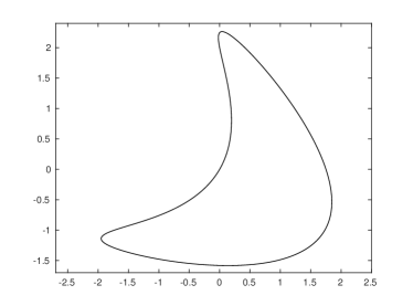
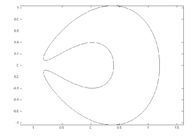
Figure 2: Kite and cavity geometries considered in the numerical experiments

For brevity, we only present numerical results for the Costabel-Stephan formulation ${\cal L}_{2}$. We refer the reader to [1, 3] for extensive numerical results for the other formulations.

$$\begin{array}[]{c|c|c|c|c}&\lx@intercol\hfil\rm Kite\hfil\lx@intercol\vrule\lx@intercol&\lx@intercol\hfil\rm Cavity\hfil\lx@intercol\\ \hline\cr&&&\\[-8.61108pt] N&{{\cal L}}_{2,N}&\widetilde{{\cal L}}_{2,N}&{{\cal L}}_{2,N}&\widetilde{{\cal L}}_{2,N}\\[4.30554pt] \hline\cr&&&\\[-8.61108pt] 96&3.2{\rm E}-02&9.1{\rm E}-03&7.1{\rm E}-02&1.7{\rm E}-02\\[4.30554pt] 128&4.1{\rm E}-04&2.5{\rm E}-05&8.3{\rm E}-04&6.3{\rm E}-05\\[4.30554pt] 160&5.9{\rm E}-11&5.8{\rm E}-12&2.0{\rm E}-10&3.3{\rm E}-11\end{array}$$

Table 1: $L^{\infty}$ error estimate in the far field for the discretizations ${{\cal L}}_{2,N}$ and $\widetilde{{\cal L}}_{2,N}$ for the Helmholtz transmission problem in the kite (left) and cavity (right) domains.

The domains we have considered are the geometries depicted in Figure 2. We have taken $k_{+}=8,k_{-}=32$ in the Helmholtz transmission problems (1), with $\nu=1$ in the transmission conditions across the interface. We have applied the numerical schemes $\widetilde{\cal L}_{2,N}$ and ${\cal L}_{2,N}$. The latter scheme is that defined using ${\rm V}_{\pm,N}$, the less accurate approximation for ${\rm V}_{\pm}$. We point out that only the first discretization has been analyzed in this paper.

The $L^{\infty}$ error estimate in the far field for the numerical solutions is shown in Table 1. The exact solution has been computed using ${\cal L}_{1,N}$ for sufficiently large $N$, which, in turns, provides an indirect demonstration of the performance of this discretization too.

Both methods converge superalgebraically to the exact solution, although $\widetilde{\cal L}_{2,N}$ performs better with even a slightly faster convergence. Convergence, and specially stability of ${\cal L}_{2,N}$ remains as an open problem and certainly will deserve more research in the future.

Acknowledgments

Catalin Turc gratefully acknowledge support from NSF through contract DMS-1312169. Víctor Domínguez is partially supported by Ministerio de Economía y Competitividad, through the grant MTM2014-52859.

References

- [1] Y. Boubendir, V. Domínguez, and C. Turc. High-order Nyström discretizations for the solution of integral equation formulations of two-dimensional Helmholtz transmission problems. To appear in IMA J. Numer. Anal.
- [2] M. Costabel and E. Stephan. A direct boundary integral equation method for transmission problems. J. Math. Anal. Appl. 106 (1985), no 2, 367–413.
- [3] V. Domínguez, M. Lyon, and C. Turc. High-order Nyström discretizations for the solution of integral equation formulations of two-dimensional Helmholtz transmission on interfaces with corners. Submitted. Preprint available in arXiv:1509.04415
- [4] R. E. Kleinman and P. A. Martin. On single integral equations for the transmission problem of acoustics. SIAM J. Appl. Math., 48 (1988), no 2, 307–325.
- [5] R. Kress and G. F. Roach. Transmission problems for the Helmholtz equation. J. Mathematical Phys., 19(6):1433–1437, 1978.
- [6] R. Kress. On the numerical solution of a hypersingular integral equation in scattering theory. J. Comput. Appl. Math. 61 (1995), no 3, 345–360.
- [7] R. Kress. Linear integral equations. Springer-Verlag, New York, third edition, 2014.
- [8] R. Kussmaul. Ein numerisches Verfahren zur Losung des Neumannschen Aussenraumproblems fur die Helmholtzsche Schwingungsgleichung. Computing 4 (1969), 246–273.
- [9] A.W. Maue.Zur Formulierung eines allgemeinen Beugungsproblems durch eine Integralgleichung. Z. Phys. 126 (1949), 601–618
- [10] E. Martensen. Uber eine Methode zum raumlichen Neumannschen Problem mit einer ANwendung fur torusartige Berandungen, Acta Math. 109 (1963), 75–135.
- [11] J.-C Nédélec. Integral equations with nonintegrable kernels. Integral Equations Operator Theory 5 (1982), no 4, 562–572.
- [12] J.-C Nédélec and J. Planchard. Une méthode variationnelle d’éléments finis pour la résolution numérique d’un problème extérieur dans . Rev. Française Automat. Informat. Recherche Opérationnelle Sér. Rouge 7 (1973), 105-129.
- [13] J. Saranen and G. Vainikko. Periodic integral and pseudodifferential equations with numerical approximation. Springer-Verlag, Berlin, 2002.