Random Projections through multiple optical scattering: Approximating kernels at the speed of light

Abstract

Random projections have proven extremely useful in many signal processing and machine learning applications. However, they often require either to store a very large random matrix, or to use a different, structured matrix to reduce the computational and memory costs. Here, we overcome this difficulty by proposing an analog, optical device, that performs the random projections literally at the speed of light without having to store any matrix in memory. This is achieved using the physical properties of multiple coherent scattering of coherent light in random media. We use this device on a simple task of classification with a kernel machine, and we show that, on the MNIST database, the experimental results closely match the theoretical performance of the corresponding kernel. This framework can help make kernel methods practical for applications that have large training sets and/or require real-time prediction. We discuss possible extensions of the method in terms of a class of kernels, speed, memory consumption and different problems.

I Introduction

Random projections have proven useful in signal processing and machine learning in several ways. A first line of applications is concerned with dimensionality reduction bingham2001random ; fradkin2003experiments ; achlioptas2003database ; hegde2008random . Given a dataset with a very large number of features, we look for a simple transformation of the data that reduces the number of features while approximately preserving the pairwise distances between data points. It turns out that linear random projection are suitable to this purpose (Johnson-Lindenstrauss lemma johnson1984extensions ). Similarly, a small number of random projections of sparse signals can carry sufficient information for their reconstruction, as shown in compressed sensing candes2006stable ; donoho2006compressed .

Conversely, non-linear random projections allow the embedding of a dataset in a larger dimensional feature space. Notably, the data may become linearly separable in this larger space, while it was not in the native feature space. A linear model can then be used to fit or classify the data. An interesting class of methods relying on this embedding is that of so-called kernel machines shawe2004kernel , among which is the celebrated SVM. These offer the advantage, sometimes called kernel trick, of not requiring the explicit mapping, but only the inner products of all pairs of embedded data points, i.e. a function $k(x,y)$ where $k$ is called the kernel, and $x,y$ are data points in the native feature space. While removing the dependency on the dimension of the embedding (which is possibly infinite), this trick relies on a matrix storing all the values of $k$ for all pairs of data points. This typically does not scale to large datasets.

Recently rahimi2007random , a cure has been proposed to this problem that actually makes explicit a non-linear mapping of the data points such that the inner product of two transformed data points approximately equals their kernel evaluation. In this new feature space, the regression or classification task can be solved by a linear machine, which can be trained very quickly compared to non-linear ones joachims2006training . Random projections have thus made some large-scale machine learning problems tractable, to the point that actually computing them - i.e. generating and storing a large random matrix, and computing matrix-vector products - has become one of the major bottlenecks in the above mentioned approaches ailon2009fast ; le2013fastfood ; meng2013low .

In this study, we demonstrate experimentally that an optical-based hardware can be built which instantaneously provides a large number of “ideal” random projections of any input data. We show that this physical process mimics, for the goal of classification, the computation of a well-defined elliptic kernel. In other words, we believe that this optical setup can be seen as a generic digital data pre-processor, for many subsequent uses of the data. It has to be emphasized that, contrary to previous studies on imaging techniques based on multiple scattering (with a similar experimental setup liutkus2014imaging ; dremeau2015reference ), this random transformation does not have to be precisely determined through a lengthy calibration stage : the knowledge of its statistical properties is enough to guarantee its effectiveness. Although this process is fundamentally analog, we show here that the associated experimental noise does not substantially change the results, which are in very good agreement with computer simulations.

II Random projections and kernel machine learning

Let us start by introducing the standard ridge regression problem, arguably the simplest kernel method for supervised classification. Throughout the section, we are given a training set composed of labeled data, represented by a matrix ${\bf U}\in\mathbb{R}^{n\times p}$ where $n$ is the number of samples and $p$ is the dimension of the data (number of features). Each data point ${\bf U}_{i}\in\mathbb{R}^{p}$ has a unique label $l_{i}\in\llbracket 1,q\rrbracket$ which we encode in a matrix ${\bf Y}\in\mathbb{R}^{n\times q}$ with elements ${\bf Y}_{i,j}=\delta_{j,l_{i}}$. We are also given a test set of unlabeled data, represented by a matrix ${\bf\tilde{U}}\in\mathbb{R}^{\tilde{n}\times p}$ where $\tilde{n}$ is the number of unlabeled samples. Our goal is to estimate their label $\tilde{{\bf Y}}\in\mathbb{R}^{\tilde{n}\times q}$ using a classifier trained on the training set. Recall that the ridge regression problem reads

$$\underset{\beta\in\mathbb{R}^{p\times q}}{\rm argmin}\ ||{\bf U}\beta-{\bf Y}||_{2}^{2}+\gamma||\beta||_{2}^{2}$$ (1)

where $\gamma$ controls the trade-off between the estimation error and the regularization. Its closed-form solution is given by

$$\beta=({\bf U}^{T}{\bf U}+\gamma{\bf I}_{p})^{-1}{\bf U}^{T}{\bf Y}={\bf U}^{T}({\bf U}{\bf U}^{T}+\gamma{\bf I}_{n})^{-1}{\bf Y}$$ (2)

where we have used a classical algebraic identity. Our prediction for the labels of the test data points is then

$${\bf\tilde{Y}}={\bf\tilde{U}}\beta ={\bf\tilde{U}}({\bf U}^{T}{\bf U}+\gamma{\bf I}_{p})^{-1}{\bf U}^{T}{\bf Y}$$ (3)

$$={\bf\tilde{U}}{\bf U}^{T}({\bf U}{\bf U}^{T}+\gamma{\bf I}_{n})^{-1}{\bf Y}$$ (4)

More precisely, since we are interested in classification, we will set the label of ${\bf\tilde{U}}_{i}$ to $\tilde{l}_{i}=\max_{j\in\llbracket 1,q\rrbracket}{\bf\tilde{Y}}_{ij}$. Note that Eq. (4) only depends on inner products of the data points.

II.1 Kernel classification

Given a kernel $k$, we define the $n\times n$ (resp. $\tilde{n}\times n$) kernel matrix ${\bf K}$ (resp. ${\bf\tilde{K}})$ with elements

$${\bf K}_{i,j}=k({\bf U}_{i},{\bf U}_{j})~{}~{}\text{and}~{}~{}{\bf\tilde{K}}_{i,j}=k({\bf\tilde{U}}_{i},{\bf U}_{j})$$ (5)

In the kernel ridge regression problem, we simply replace the Euclidean inner product in feature space by this kernel. Because Eq. (4) only depends on these inner products, we do not have to explicit the mapping, and the solution of the kernel ridge regression is directly given by

$$\tilde{\bf Y}=\tilde{\bf K}({\bf K}+\gamma{\bf I}_{n})^{-1}{\bf Y}$$ (6)

We consider here the following elliptic kernel:

$$k({\bf U}_{i},{\bf U}_{j}) =\frac{\sqrt{{\bf U}_{i}^{T}{\bf U}_{i}\,{\bf U}_{j}^{T}{\bf U}_{j}}}{2}\Bigg{\{}-(\sin^{2}\theta){\cal E}_{K}\left[\cos^{2}\theta\right]+2{\cal E}_{E}\left[\cos^{2}\theta\right]\negmedspace+\negmedspace|\sin{\theta}|\left(2{\cal E}_{E}\negmedspace\left[-\frac{\cos^{2}\theta}{\sin^{2}\theta}\right]\negmedspace-\negmedspace{\cal E}_{K}\negmedspace\left[-\frac{\cos^{2}\theta}{\sin^{2}\theta}\right]\right)\!\!\!\Bigg{\}}$$ (7)

where ${\cal E}_{K}[.]$ and ${\cal E}_{E}[.]$ are the complete elliptic integrals of the first and second kind respectively, and $\theta$ the angle between ${\bf U}_{i}$ and ${\bf U}_{j}$. Despite its apparent complexity, this function essentially looks like a bell curve as a function of $\theta$, and therefore quantifies the similarity between ${\bf U}_{i}$ and ${\bf U}_{j}$. This particular choice will be motivated experimentally in section II.3.

To illustrate this method, we consider the MNIST dataset of handwritten digits lecun1998gradient . This dataset is split into a training set of $60000$ digits of size $28\times 28$, and a test set of $10000$ digits. Using the elliptic kernel, we achieve a classification error of $1.31\%$, to be compared with a $12\%$ error for the purely linear ridge regression (4). While better results can be achieved using much more complex deep neural networks, kernel ridge regression achieves a reasonable error and is remarkable in its simplicity. The major drawback of this approach is the computational cost of inverting an $n\times n$ matrix. In “big data” problems, where $n$ can be in the billions, it would not even be possible to store such a matrix.

II.2 Random projections

Following rahimi2007random , we now compute a non-linear mapping and solve the linear ridge regression problem (1) in this new feature space of dimension $N$. Specifically, we consider mappings of the form

$${\bf X}_{i,j}=\phi(({\bf WU}_{i})_{j}+{\bf b}_{j})\qquad i\in\llbracket 1,n\rrbracket,j\in\llbracket 1,N\rrbracket$$ (8)

where ${\bf b}$ is a bias, $\phi$ is a non-linear function and ${\bf W}\in\mathbb{R}^{N\times p}$ is a linear projection which we take to be random. The solution of the ridge regression problem is

$$\tilde{\bf Y}\negmedspace=\negmedspace{\bf\tilde{X}}{\bf X}^{T}\negmedspace({\bf X}{\bf X}^{T}\negmedspace+\negmedspace\gamma{\bf I}_{n})^{-1}{\bf Y}\negmedspace=\negmedspace{\bf\tilde{X}}({\bf X}^{T}{\bf X}\negmedspace+\negmedspace\gamma{\bf I}_{N})^{-1}{\bf X}^{T}{\bf Y}\negmedspace$$ (9)

In this last formulation, we see that if the inner products of the data points in the new feature space approximate a kernel, and if this new feature space has a reasonable dimension $N$, then we can approximate a kernel ridge regression by inverting a smaller matrix (${\bf X}^{T}{\bf X}\in\mathbb{R}^{N\times N}$) instead of the kernel matrix (${\bf X}{\bf X}^{T}\in\mathbb{R}^{n\times n}$). Concretely, the experimental device described in the next section can perform (8) with ${\bf W}$ a random i.i.d complex matrix with Gaussian real and imaginary parts, $\phi$ the modulus function, and a vanishing bias ${\bf b}$. This setting has been popularized recently under the name Extreme Learning Machine huang2006extreme ; huang2004extreme . In synthetic experiments, if we use $N=10000$ random projections and the linear ridge regression (9), we get an error of approximately $2\%$ (see Fig. 1), having only to invert a $10000^{2}$ matrix instead of a $60000^{2}$ one. Even better: now we have lost the dependency on $n^{2}$.

II.3 Random complex projections and the elliptic kernel

In the limit where the number of projections $N$ grows to infinity, due to the concentration of the measure, it is possible to show that the inner product between the projected data points ${\bf X}_{i}\in\mathbb{R}^{N}$ tends to a kernel function that depends only on the ${\bf U}_{i}$ williams1998computation . With the choice of ${\bf W}$ and $\phi$ corresponding to our experiment, a tedious but simple computation shows that the limiting kernel is precisely the elliptic kernel of equation (7). To approximate this kernel, we can therefore use our experimental device to perform the non-linear projections, and solve the ridge regression problem (9). This concentration phenomenon is shown on Fig. 1 where we plot the classification error on the MNIST database when the number of random projections is increased (red points). As the number of random projections grows, the classification error using synthetic random projections approaches the asymptotic value using the true elliptic kernel ($1.31\%$). Empirically, we find that these corrections are very well fitted by a power law in $N^{-2/3}$.

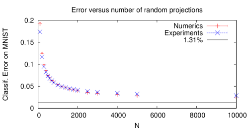
Figure 1: Comparison between synthetic random projections and the experimental ones. The classification error is shown as a function of the dimension $N$ of the feature space. As $N$ increases, the error using synthetic random projections (red) approaches the asymptotic value using the true elliptic kernel (here $1.31\%$). Experimental results, made with our optical device, closely follow the synthetic ones though they tend to deviate from the synthetic data for larger $N$ (see discussion).

III Experimental Apparatus

The approach exposed in the previous section still requires to store, and multiply by, a potentially huge random matrix, and to apply the modulus function. We now move to the discussion of our experimental apparatus which will make this procedure a trivial, instantaneous one.

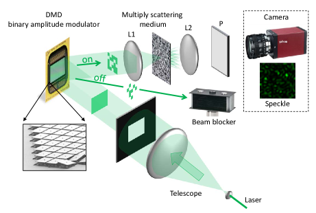
Figure 2: Experimental setup (from dremeau2015reference ). A monochromatic laser at 532nm is expanded by a telescope, then illuminates a digital micromirror device (DMD), able to spatially encode digital information on the light beam by amplitude modulation, as described in section III.2. The light beam carrying the signal is then focused on a random medium by means of a lens. Here, the medium is a thick (several tens of microns) layer of $TiO_{2}$ (Titanium Dioxide) nanoparticles (white paint pigments deposited on a microscope glass slide). The transmitted light is collected on the far side by a second lens, passes through a polarizer, and is measured by a standard monochrome CCD camera.

III.1 Principle of optical analog random projections

At the basis of the analog random projections, we exploit the ability of a heterogeneous material, such as paper, paint, or any white translucid material, to scatter light impinging on them in a very complex way. Due to their extremely high complexity, their behavior for light scattering is considered “random”, and this kind of medium are often called “random medium”. This term is abusive since scattering is a linear, deterministic, and reproducible phenomenon. However, the unpredictable nature of the process makes it effectively a random process. This is why these materials are called “opaque”, since all information on the incoming light is seemingly lost (but only irremediably mixed) during the propagation. As an example, consider a cube of edge size 100 $\mu$m. It comprises $\approx 10^{7}$ paint nanoparticles, whose positions and shape would have to be exactly known in order to predict its effect on light. Propagation through such a layer can be seen as a random walk because of frequent scattering with the nanoparticles. The characteristic step is the transport mean free path, typically of a few $\mu$m, so light would explore the whole volume and endure on average tens of thousands of such steps before exiting on the other side, in a few picoseconds.

When light is coherent, it gives rise to interferences. The complex interference pattern arising from the multiple scattering process is called “speckle”. It is characteristic not only of the heterogeneous material, but also of the “shape” of the input light. In essence, the propagation of light through a random medium can be modeled as $y={\bf H}x$ where $y$ (resp. $x$) are vector amplitudes between a set of spatial modes at the output (resp. input) of the medium, and where ${\bf H}$ is the so-called transmission matrix of the medium, which has been shown to be very close to Gaussian i.i.d matrices popoff2010measuring . By “interrogating” the medium with an appropriate set of input illuminations, which can be conveniently done using a spatial light modulator and a laser, and measuring the resulting “answer” by means of a CCD or CMOS camera for instance, one would therefore record the resulting intensity $\lvert y\rvert^{2}$ (see Fig. 2). For a stable medium, such as a paint layer for instance, the transmission matrix ${\bf H}$ is stable and the medium can therefore provide a convenient platform for random projections, without the need to determine ${\bf H}$.

III.2 Encoding the data on the DMD

The DMD we use is a $1920\times 1080$ array of micro-mirrors. Each micro-mirror encodes a binary value (lit or not). Levels of grey can be conventionally coded in time by lighting up a micro-mirror for a fraction of the exposure time of the camera. This approach however reduces the frequency at which data can be processed through the apparatus. We therefore resorted to spatial encoding. We encoded each pixel of an image on a $4\times 4$ array of micro-mirrors in which the number of lit micro-mirrors reflects the level of grey of the pixel. This allowed us to encode $17$ grey levels.

Each digit in the MNIST dataset can be seen as a $28^{2}$ array of integers between $0$ and $255$. We first quantized the grey levels between $0$ and $16$. We then encoded each of these quantized pixels as a $4\times 4$ array of micro-mirrors. This results in a $112^{2}$ array of binary variables. To rescale the resulting image to $1920\times 1080$, which is the size of the DMD, we need to first add a border of zeros, so that the image becomes of size $120^{2}$. Finally, we can rescale the image by a factor of $16\times 9$. The result is a $1920\times 1080$ binary image, encoding each digit over $17$ levels of grey. This image can then be projected on the DMD. It is in principle possible to encode more levels of grey by encoding each pixel on a larger array of micro-mirrors. The procedure described to encode the data on the DMD is not specific to images and generalizes to any kind of data which can be written as a numerical vector.

After sending the data through the disordered medium, we acquire a snapshot of the resulting random projection using a standard camera. To reduce the correlations between neighboring pixels of the output, we start by acquiring a $400^{2}$ pixel area, which we then reduce to $100^{2}$ pixels where each of these pixels is the average of a $4^{2}$ patch in the original snapshot.

IV Results

Our results are summarized in Fig. 1 where we compare the efficiency in classification using synthetic random projection (in red) and the random projection obtained within the experimental set-up (in blue). We find that the two curves agree remarkably well, thus validating our procedure to generate analog random projections for classification tasks.

We note, however, that when the number of projections is increased to large values, i.e. $N\gtrsim 2000$, the optical experiment starts to deviate from the synthetic one. We checked numerically that adding even large noise to the synthetic projection did not change the results of the classification, which is therefore robust to experimental noise. We thus believe that this deviation is due to residual correlations between pixels of the output image. The number of independent pixels can be tuned in several ways, for instance by ensuring that the CCD pixel on the output camera matches the size of a speckle grain, or by tuning the thickness of the random medium itself to increase the number of independent modes popoff2010measuring . We are therefore confident that this deviation can be decreased with further development of the experimental apparatus.

V Conclusion and perspectives

This study shows that large dimensional (here $10^{4}$ - $10^{6}$) random projections of digital data can be obtained almost instantaneously with an optical device, that can then be used for practical machine learning applications such as (but not limited to) kernel classification. The speed of “computation” is only limited by how fast one can modulate light at the input (off-the-shelf DMDs can handle images with millions of pixels, at rates of $20$ kHz or above), and measure the corresponding scattered light. Note also that although optical sensors natively measure only the intensity (squared modulus) of the field, and not the complex-valued field itself, this is precisely what is needed for the kernel computations presented here, akin to the non-linear transform of each layer of a neural network. In the cases where the linear projections are needed, e.g. for randomized linear algebra, the experimental setup can be modified to include an interferometric arm. We can then apply any non-linear function using e.g. FPGAs, widening the range of kernels we can approximate. It is also possible to combine several DMDs together to process larger signals.

More generally, we believe that this experiment is a first proof-of-concept toward a new generation of analog optical-based co-processors, able to complement existing silicon-based chips for the processing of very large datasets, with potential benefits in terms of data throughput and energy consumption.

References

- [1] Dimitris Achlioptas. Database-friendly random projections: Johnson-lindenstrauss with binary coins. Journal of computer and System Sciences, 66(4):671–687, 2003.
- [2] Nir Ailon and Edo Liberty. Fast dimension reduction using rademacher series on dual bch codes. Discrete & Computational Geometry, 42(4):615–630, 2009.
- [3] Ella Bingham and Heikki Mannila. Random projection in dimensionality reduction: applications to image and text data. In Proceedings of the seventh ACM SIGKDD international conference on Knowledge discovery and data mining, pages 245–250. ACM, 2001.
- [4] Emmanuel J Candes, Justin K Romberg, and Terence Tao. Stable signal recovery from incomplete and inaccurate measurements. Communications on pure and applied mathematics, 59(8):1207–1223, 2006.
- [5] David L Donoho. Compressed sensing. Information Theory, IEEE Transactions on, 52(4):1289–1306, 2006.
- [6] Angélique Drémeau, Antoine Liutkus, David Martina, Ori Katz, Christophe Schülke, Florent Krzakala, Sylvain Gigan, and Laurent Daudet. Reference-less measurement of the transmission matrix of a highly scattering material using a dmd and phase retrieval techniques. Optics express, 23(9):11898–11911, 2015.
- [7] Dmitriy Fradkin and David Madigan. Experiments with random projections for machine learning. In Proceedings of the ninth ACM SIGKDD international conference on Knowledge discovery and data mining, pages 517–522. ACM, 2003.
- [8] Chinmay Hegde, Michael Wakin, and Richard Baraniuk. Random projections for manifold learning. In Advances in neural information processing systems, pages 641–648, 2008.
- [9] Guang-Bin Huang, Qin-Yu Zhu, and Chee-Kheong Siew. Extreme learning machine: a new learning scheme of feedforward neural networks. In Neural Networks, 2004. Proceedings. 2004 IEEE International Joint Conference on, volume 2, pages 985–990. IEEE, 2004.
- [10] Guang-Bin Huang, Qin-Yu Zhu, and Chee-Kheong Siew. Extreme learning machine: theory and applications. Neurocomputing, 70(1):489–501, 2006.
- [11] Thorsten Joachims. Training linear svms in linear time. In Proceedings of the 12th ACM SIGKDD international conference on Knowledge discovery and data mining, pages 217–226. ACM, 2006.
- [12] William B Johnson and Joram Lindenstrauss. Extensions of lipschitz mappings into a hilbert space. Contemporary mathematics, 26(189-206):1, 1984.
- [13] Quoc Le, Tamás Sarlós, and Alex Smola. Fastfood-approximating kernel expansions in loglinear time. In Proceedings of the international conference on machine learning, 2013.
- [14] Yann LeCun, Léon Bottou, Yoshua Bengio, and Patrick Haffner. Gradient-based learning applied to document recognition. Proceedings of the IEEE, 86(11):2278–2324, 1998.
- [15] Antoine Liutkus, David Martina, Sébastien Popoff, Gilles Chardon, Ori Katz, Geoffroy Lerosey, Sylvain Gigan, Laurent Daudet, and Igor Carron. Imaging with nature: Compressive imaging using a multiply scattering medium. Scientific reports, 4, 2014.
- [16] Xiangrui Meng and Michael W Mahoney. Low-distortion subspace embeddings in input-sparsity time and applications to robust linear regression. In Proceedings of the forty-fifth annual ACM symposium on Theory of computing, pages 91–100. ACM, 2013.
- [17] SM Popoff, G Lerosey, R Carminati, M Fink, AC Boccara, and S Gigan. Measuring the transmission matrix in optics: an approach to the study and control of light propagation in disordered media. Physical review letters, 104(10):100601, 2010.
- [18] Ali Rahimi and Benjamin Recht. Random features for large-scale kernel machines. In Advances in neural information processing systems, pages 1177–1184, 2007.
- [19] John Shawe-Taylor and Nello Cristianini. Kernel methods for pattern analysis. Cambridge university press, 2004.
- [20] Christopher KI Williams. Computation with infinite neural networks. Neural Computation, 10(5):1203–1216, 1998.