Replica-symmetric approach to the typical eigenvalue fluctuations of Gaussian random matrices

Abstract

We discuss an approach to compute the first and second moments of the number of eigenvalues $I_{N}$ that lie in an arbitrary interval of the real line for $N\times N$ Gaussian random matrices. The method combines the standard replica-symmetric theory with a perturbative expansion of the saddle-point action up to $O(1/N)$ ($N\gg 1$), leading to the correct logarithmic scaling of the variance $\langle I_{N}^{2}\rangle-\langle I_{N}\rangle^{2}=O(\ln N)$ as well as to an analytical expression for the $O(1/N)$ correction to the average $\langle I_{N}\rangle/N$. Standard results for the number variance at the local scaling regime are recovered in the limit of a vanishing interval. The limitations of the replica-symmetric method are unveiled by comparing our results with those derived through exact methods. The present work represents an important step to study the fluctuations of $I_{N}$ in non-invariant random matrix ensembles, where the joint distribution of eigenvalues is not known.

1 Introduction

In the last decades, random matrices have established itself as a fundamental tool to model complex disordered systems, with many applications in different branches of science [1, 2]. The primary aim in random matrix theory is the study of the eigenvalue statistics, which is accessed by computing suitably chosen observables. Important observables are the moments of the number of eigenvalues $I(a,b)$ that lie between $a\in\mathbb{R}$ and $b\in\mathbb{R}$. For $a\rightarrow-\infty$, the random variable $I$ is the so-called index, i.e., the number of eigenvalues contained in the unbounded interval $(-\infty,b]$. A great deal of attention has been devoted to the index of random matrices, especially due to its ability to probe the stability properties of the energy landscape characterising disordered systems [3, 4]. Another prominent observable, derived from $I(a,b)$ and studied originally by Dyson [5], is the variance of the number of eigenvalues within the bounded interval $[-L,L]$ ($L>0$), also known as the number variance. Recently, this observable has been applied to study the statistics of non-interacting fermions confined in a harmonic trap [6, 7], and the ergodicity of the eigenfunctions in a mean-field model for the Anderson localisation transition [8, 9].

A powerful tool to study the fluctuations of $I(a,b)$ is the Coulomb gas approach [10], whose starting point is an exact correspondence between the joint distribution of eigenvalues and the partition function of a two-dimensional Coulomb gas confined to a line. The Coulomb gas technique has been employed to derive analytical results for typical and atypical fluctuations of $I(a,b)$ in the case of rotationally invariant random matrices (RIRM), including Gaussian [6, 7, 11, 12, 13, 14], Wishart [15, 16] and Cauchy [17] random matrices. Restricting ourselves to typical fluctuations of $I$, one of the central outcomes for RIRM is the logarithmic increase of the variance $\langle I^{2}\rangle-\langle I\rangle^{2}\propto\ln N$ as a function of the matrix dimension $N\gg 1$, due to the strong correlations among the eigenvalues. In spite of the success of the Coulomb gas method, its application is strictly limited to RIRM, where the joint distribution of eigenvalues is analytically known and, consequently, the analogy with the Coulomb gas partition function can be readily established.

Recently, a novel technique to study the fluctuations of $I(a,b)$ has been developed [8, 18]. This method is based on the replica-symmetric theory of disordered systems and its main advantage lies in its broad range of possible applications, which goes beyond the realm of RIRM. In fact, the replica approach allows to derive analytical results for typical and atypical fluctuations of $I(a,b)$ in the case of random matrices where the joint distribution of eigenvalues is not even known. The most typical example in this sense is the adjacency matrix of sparse random graphs [8, 18], where the eigenvalues behave as uncorrelated random variables and the leading term of the variance scales as $\langle I^{2}\rangle-\langle I\rangle^{2}\propto N$ for large $N$. However, it is unclear whether the formalism of [8, 18] is able to grasp the variance behaviour $\langle I^{2}\rangle-\langle I\rangle^{2}\propto\ln N$ of random matrices with strong correlated eigenvalues. In the case of a positive answer, this would pave the way to inspect the fluctuations of $I$ in random matrices that are not rotationally invariant, but in which the eigenvalues are strongly correlated. The ensembles of Gaussian random matrices are the ideal testing ground for this matter, since one can make detailed comparisons with exact results and identify eventual limitations of the replica method.

In this work we show how the replica approach, as developed in [18, 8], has to be further adapted in order to derive the correct logarithmic scaling $\langle I^{2}\rangle-\langle I\rangle^{2}\propto\ln N$ for the GOE and the GUE ensembles of random matrices [10, 1]. Following the approach of [19], the central idea here consists in writing the characteristic function of $I$ as a saddle-point integral, in which the action is computed perturbatively around its $N\rightarrow\infty$ limit. We show that the leading term $\langle I^{2}\rangle-\langle I\rangle^{2}\propto\ln N$ ($N\gg 1$) is correctly recovered only when the fluctuations due to finite $N$ are taken into account. However, the present approach does not yield the exact expression for the $O(N^{0})$ contribution to the variance of $I$, due to our assumption of replica-symmetry for the order-parameter. In the case of the number variance, our analytical expression converges, in the limit $L\rightarrow 0^{+}$, to standard results of random matrix theory [1], valid in the regime where the spectral window is measured in units of the mean level spacing. This result supports the central claim of reference [9], where the limit $L\rightarrow 0^{+}$ of the number variance is employed to study the ergodic nature of the eigenfunctions in the Anderson model on a regular random graph. As a by-product, our method yields the $O(1/N)$ correction to the intensive average $\langle I\rangle/N$, whose exactness is tested against numerical diagonalisation and previous analytical results. While the $O(1/N)$ contribution to $\langle I\rangle/N$ is exact for the GOE ensemble, it fails in the case of the GUE ensemble due to our assumption of replica symmetry. The present approach can be also employed to compute the moments of characteristic polynomials of non-invariant random matrices, where the key quantity under study is similar to eq. (7). The moments of characteristic polynomials of invariant random matrices have been largely studied [20, 21, 22], in view of their connection with the distribution of zeros of the Riemann zeta function [23].

The paper is organised as follows. In the next section we show how the computation of the characteristic function of $I$ can be pursued using the replica approach. Section 3 explains the basic steps of the replica method, including the perturbative calculation of the action up to $O(1/N)$. We make the replica-symmetric assumption for the order-parameter and derive an analytical expression for the characteristic function in section 4. Section 5 derives the analytical results for the index, the number variance and the fluctuations of $I$ in an arbitrary interval. The last section summarises our work and discusses the impact of replica symmetry in our results.

2 The number of eigenvalues inside an interval

We study here two different ensembles of $N\times N$ Gaussian random matrices $M$ with real eigenvalues $\lambda_{1},\dots,\lambda_{N}$, defined through the probability distribution $\mathcal{P}(\mbox{\boldmath$M$})$. If the elements of the ensemble are real symmetric matrices, we have the Gaussian orthogonal ensemble (GOE) [1]

$$\mathcal{P}(\mbox{\boldmath$M$})=\mathcal{N}_{GOE}\exp{\left(-\frac{N}{4}\Tr\mbox{\boldmath$M$}^{2}\right)}\,.$$ (1)

If the ensemble is composed of complex-Hermitian random matrices, we have the Gaussian unitary ensemble (GUE) [1]

$$\mathcal{P}(\mbox{\boldmath$M$})=\mathcal{N}_{GUE}\exp{\left[-\frac{N}{2}\Tr\left(\mbox{\boldmath$M$}^{\dagger}\mbox{\boldmath$M$}\right)\right]}\,,$$ (2)

where $(\dots)^{\dagger}$ represents the conjugate transpose of a matrix. The explicit form of the normalization factors in eqs. (1) and (2) are not important in our computation.

The number of eigenvalues $I_{N}(a,b)$ lying between $a\in\mathbb{R}$ and $b\in\mathbb{R}$ is given by

$$I_{N}(a,b)=\sum_{\alpha=1}^{N}\left[\Theta(b-\lambda_{\alpha})-\Theta(a-\lambda_{\alpha})\right]\quad a<b,$$ (3)

with $\Theta(\dots)$ the Heaviside step function. The statistics of $I_{N}(a,b)$ is encoded in the characteristic function

$$\mathcal{G}_{N}(\mu)=\langle\exp{\left[i\mu I_{N}(a,b)\right]}\rangle,$$ (4)

where $\langle\dots\rangle$ is the ensemble average over the random matrix elements. In particular, the first two moments of $I_{N}(a,b)$ read

$$\langle I_{N}(a,b)\rangle=-i\frac{\partial\mathcal{G}_{N}(\mu)}{\partial\mu}\Big{|}_{\mu=0},\qquad\langle I_{N}^{2}(a,b)\rangle=-\frac{\partial^{2}\mathcal{G}_{N}(\mu)}{\partial\mu^{2}}\Big{|}_{\mu=0}.$$ (5)

In order to calculate the ensemble average in eq. (4), one has to write $I_{N}(a,b)$ in terms of the random matrix $M$. By following [3, 18] and representing $\Theta$ as the discontinuity of the principal value of the complex logarithm along the negative real axis, $I_{N}(a,b)$ may be written as the limit

$$I_{N}(a,b)=\frac{1}{2\pi i}\lim_{\eta\rightarrow 0^{+}}\ln{\left[\frac{Z(z_{b})Z(z^{*}_{a})}{Z(z^{*}_{b})Z(z_{a})}\right]},\qquad z_{a}=a+i\eta\,,\qquad z_{b}=b+i\eta\,,$$ (6)

with $Z(z)=\left[\det{\left(\mbox{\boldmath$M$}-z\mbox{\boldmath$I$}_{N}\right)}\right]^{-1}$. Here $z$ is an arbitrary complex number, $z^{*}$ denotes its complex-conjugate, and $\mbox{\boldmath$I$}_{N}$ is the $N\times N$ identity matrix. Since the imaginary part of the principal logarithm is bounded in $(-\pi,\pi]$, the right hand side of eq. (6) is not extensive and, consequently, unfit to count the number of eigenvalues within $[a,b]$ for single realizations of $M$. This issue comes from our naive derivation of eq. (6), where we assume that the principal complex logarithm fulfills the same standard properties as those valid for the logarithm of real numbers. In spite of that, this is a necessary step to apply the replica method. We will see that, after calculating the ensemble average and introducing an appropriate order-parameter, the problem factorises over sites and the extensivity of the moments of $I_{N}(a,b)$ is restored. This procedure is heuristic, but it yields correct results for the moments of $I_{N}(a,b)$ for large $N$. Thus, eq. (6) completely encodes the statistics of $I_{N}(a,b)$, even though it is unsuitable to obtain $I_{N}(a,b)$ for single instances of $M$.

Inserting eq. (6) in eq. (4), we find

$$\mathcal{G}_{N}(\mu)=\lim_{\eta\rightarrow 0^{+}}\left\langle\left[Z(z_{b})Z(z_{a}^{*})\right]^{\frac{\mu}{2\pi}}\left[Z(z_{b}^{*})Z(z_{a})\right]^{-\frac{\mu}{2\pi}}\right\rangle.$$ (7)

At this point we invoke the replica method in the form

$$\mathcal{G}_{N}(\mu)=\lim_{\eta\rightarrow 0^{+}}\lim_{n_{\pm}\rightarrow\pm\frac{\mu}{2\pi}}\mathcal{G}_{N}(n_{\pm},\eta)\,,$$ (8)

in which we have introduced the function

$$\mathcal{G}_{N}(n_{\pm},\eta)=\left\langle\left[Z(z_{b})Z(z_{a}^{*})\right]^{n_{+}}\left[Z(z_{b}^{*})Z(z_{a})\right]^{n_{-}}\right\rangle$$ (9)

for finite $\eta$. The idea consists in assuming that $n_{\pm}$ are positive integers, which allows to calculate $\mathcal{G}_{N}(n_{\pm},\eta)$ for $N\gg 1$ through a saddle-point integration. After we have derived the behaviour of $\mathcal{G}_{N}(n_{\pm},\eta)$ for $N\gg 1$, we take the replica limit $n_{\pm}\rightarrow\pm\frac{\mu}{2\pi}$ and reconstruct the original function $\mathcal{G}_{N}(\mu)$ in the limit $\eta\rightarrow 0^{+}$. This is nothing more than the general strategy of the replica approach [24]. The only difference lies in the fact that we continue the arbitrary positive integers $n_{\pm}$ to purely imaginary numbers.

3 Replica method and finite size corrections

Our aim in this section is to calculate $\mathcal{G}_{N}(n_{\pm},\eta)$ for large but finite $N$. Firstly, we have to recast eq. (9) into an exponential form, which is suitable to perform the ensemble average. This is achieved by representing the functions $Z(z_{a,b})$ and $Z(z_{a,b}^{*})$ as Gaussian integrals. For instance, the function $Z(z_{a})$ is written as the multidimensional Gaussian integral [25]

$$Z(z_{a})=\frac{1}{\det{\left(\mbox{\boldmath$M$}-\mbox{\boldmath$I$}_{N}z_{a}\right)}}=\frac{1}{(2\pi)^{N}}\int\left(\prod_{i=1}^{N}d\phi_{i}d\phi_{i}^{*}\right)\exp{\left[-i\sum_{ij=1}^{N}\phi_{i}^{*}\left(\mbox{\boldmath$M$}-\mbox{\boldmath$I$}_{N}z_{a}\right)_{ij}\phi_{j}\right]},$$ (10)

where $\phi_{1},\dots,\phi_{N}$ are complex integration variables. This representation of $Z(z_{a})$ is appropriate to deal with both the GOE ensemble and the GUE ensemble in the same framework. Introducing analogous identities for $Z(z_{b})$, $Z(z_{b}^{*})$ and $Z(z_{a}^{*})$, eq. (9) can be compactly written as

$$\mathcal{G}_{N}(n_{\pm},\eta)=\int\left(\prod_{i=1}^{N}d\mbox{\boldmath$\varphi$}_{i}d\mbox{\boldmath$\varphi$}_{i}^{\dagger}\right)\exp{\left(i\sum_{i=1}^{N}\mbox{\boldmath$\varphi$}_{i}^{\dagger}.\mbox{\boldmath$Z$}\mbox{\boldmath$\varphi$}_{i}\right)}\left\langle\exp{\left[-i\sum_{ij=1}^{N}M_{ij}\left(\mbox{\boldmath$\varphi$}_{i}^{\dagger}.\mbox{\boldmath$A$}\mbox{\boldmath$\varphi$}_{j}\right)\right]}\right\rangle,$$ (11)

where the following $2(n_{+}+n_{-})\times 2(n_{+}+n_{-})$ block matrices have been introduced

$$\mbox{\boldmath$A$}=\left(\begin{array}[]{cccc}\mbox{\boldmath$I$}_{+}&0&0&0\\ 0&\mbox{\boldmath$I$}_{-}&0&0\\ 0&0&-\mbox{\boldmath$I$}_{+}&0\\ 0&0&0&-\mbox{\boldmath$I$}_{-}\end{array}\right),\qquad\mbox{\boldmath$Z$}=\left(\begin{array}[]{cccc}z_{b}\mbox{\boldmath$I$}_{+}&0&0&0\\ 0&z_{a}\mbox{\boldmath$I$}_{-}&0&0\\ 0&0&-z_{a}^{*}\mbox{\boldmath$I$}_{+}&0\\ 0&0&0&-z_{b}^{*}\mbox{\boldmath$I$}_{-}\end{array}\right),$$

with $\mbox{\boldmath$I$}_{+}$ ($\mbox{\boldmath$I$}_{-}$) denoting the $n_{+}\times n_{+}$ ($n_{-}\times n_{-}$) identity matrix. The integration variables in eq. (11) are $2(n_{+}+n_{-})$-dimensional complex vectors in the replica space, defined according to

$$\mbox{\boldmath$\varphi$}_{i}=\left(\begin{array}[]{c}\bm{\phi}_{1,i}\\ \bm{\psi}_{1,i}\\ \bm{\phi}_{2,i}\\ \bm{\psi}_{2,i}\end{array}\right)\qquad i=1,\dots,N,$$

where $\bm{\phi}_{1,i}$ and $\bm{\phi}_{2,i}$ have dimension $n_{+}$, while $\bm{\psi}_{1,i}$ and $\bm{\psi}_{2,i}$ have dimension $n_{-}$. Each one of the vectors $(\bm{\phi}_{1,i},\bm{\phi}_{2,i},\bm{\psi}_{1,i},\bm{\psi}_{2,i})$ comes from the Gaussian integral representation of a single function $Z(\dots)$ in eq. (9). The off-diagonal blocks of $Z$ and $A$, filled with zeros, have suitable dimensions, such that their product with $\mbox{\boldmath$\varphi$}_{i}$ is well-defined.

The ensemble average in eq. (11) is easily performed for the GOE and the GUE ensembles by using eqs. (1) and (2), leading to

$$\mathcal{G}_{N}(n_{\pm},\eta)=\int\left(\prod_{i=1}^{N}d\mbox{\boldmath$\varphi$}_{i}d\mbox{\boldmath$\varphi$}_{i}^{\dagger}\right)\exp{\left[i\sum_{i=1}^{N}\mbox{\boldmath$\varphi$}_{i}^{\dagger}.\mbox{\boldmath$Z$}\mbox{\boldmath$\varphi$}_{i}-\frac{1}{2N}\sum_{ij=1}^{N}K_{\beta}(\mbox{\boldmath$\varphi$}_{i},\mbox{\boldmath$\varphi$}_{i}^{\dagger},\mbox{\boldmath$\varphi$}_{j},\mbox{\boldmath$\varphi$}_{j}^{\dagger})\right]}\,,$$ (12)

with the kernel $K_{\beta}$

$$K_{\beta}(\mbox{\boldmath$\varphi$}_{i},\mbox{\boldmath$\varphi$}_{i}^{\dagger},\mbox{\boldmath$\varphi$}_{j},\mbox{\boldmath$\varphi$}_{j}^{\dagger})=|\mbox{\boldmath$\varphi$}_{i}^{\dagger}.\mbox{\boldmath$A$}\mbox{\boldmath$\varphi$}_{j}|^{2}+(2-\beta)\,{\rm Re}\,(\mbox{\boldmath$\varphi$}_{i}^{\dagger}.\mbox{\boldmath$A$}\mbox{\boldmath$\varphi$}_{j})^{2}\,,$$ (13)

which depends on the random matrix ensemble through the Dyson index $\beta$: $\beta=1$ for the GOE ensemble and $\beta=2$ for the GUE ensemble. Following the standard approach to decouple the sites in eq. (12), we introduce the order-parameter

$$\rho(\mbox{\boldmath$\varphi$},\mbox{\boldmath$\varphi$}^{\dagger})=\frac{1}{N}\sum_{i=1}^{N}\delta(\mbox{\boldmath$\varphi$}-\mbox{\boldmath$\varphi$}_{i})\delta(\mbox{\boldmath$\varphi$}^{\dagger}-\mbox{\boldmath$\varphi$}_{i}^{\dagger})$$ (14)

through a functional Dirac delta, yielding

$$\mathcal{G}_{N}(n_{\pm},\eta) = \int\mathcal{D}\rho\mathcal{D}\hat{\rho}\exp{\left[i\int d\mbox{\boldmath$\varphi$}d\mbox{\boldmath$\varphi$}^{\dagger}\rho(\mbox{\boldmath$\varphi$},\mbox{\boldmath$\varphi$}^{\dagger})\hat{\rho}(\mbox{\boldmath$\varphi$},\mbox{\boldmath$\varphi$}^{\dagger})\right]}$$ (15)

$$\times \exp{\left[-\frac{N}{2}\int d\mbox{\boldmath$\varphi$}_{1}d\mbox{\boldmath$\varphi$}_{1}^{\dagger}d\mbox{\boldmath$\varphi$}_{2}d\mbox{\boldmath$\varphi$}_{2}^{\dagger}\,\rho(\mbox{\boldmath$\varphi$}_{1},\mbox{\boldmath$\varphi$}_{1}^{\dagger})K_{\beta}(\mbox{\boldmath$\varphi$}_{1},\mbox{\boldmath$\varphi$}_{1}^{\dagger},\mbox{\boldmath$\varphi$}_{2},\mbox{\boldmath$\varphi$}_{2}^{\dagger})\rho(\mbox{\boldmath$\varphi$}_{2},\mbox{\boldmath$\varphi$}_{2}^{\dagger})\right]}$$

$$\times \exp{\left[N\ln{\left[\int d\mbox{\boldmath$\varphi$}d\mbox{\boldmath$\varphi$}^{\dagger}\exp{\left(i\mbox{\boldmath$\varphi$}^{\dagger}.\mbox{\boldmath$Z$}\mbox{\boldmath$\varphi$}-\frac{i}{N}\hat{\rho}(\mbox{\boldmath$\varphi$},\mbox{\boldmath$\varphi$}^{\dagger})\right)}\right]}\right]},$$

where $\mathcal{D}\rho\mathcal{D}\hat{\rho}$ is the functional integration measure over $\rho$ and its conjugate order-parameter $\hat{\rho}$. After performing the Gaussian integral over $\rho$ and introducing a new integration variable $\Phi$

$$\hat{\rho}(\mbox{\boldmath$\varphi$},\mbox{\boldmath$\varphi$}^{\dagger})=-iN\int d\mbox{\boldmath$\varphi$}_{1}d\mbox{\boldmath$\varphi$}_{1}^{\dagger}K_{\beta}(\mbox{\boldmath$\varphi$},\mbox{\boldmath$\varphi$}^{\dagger},\mbox{\boldmath$\varphi$}_{1},\mbox{\boldmath$\varphi$}_{1}^{\dagger})\Phi(\mbox{\boldmath$\varphi$}_{1},\mbox{\boldmath$\varphi$}_{1}^{\dagger})\,,$$ (16)

we obtain the compact expression

$$\mathcal{G}_{N}(n_{\pm},\eta)=\sqrt{\det{K_{\beta}}}\int\mathcal{D}\Phi\exp{\left(NS_{N}[\Phi]\right)}\,,$$ (17)

with the action:

$$S_{N}[\Phi] = \frac{1}{2}\int d\mbox{\boldmath$\varphi$}_{1}d\mbox{\boldmath$\varphi$}_{1}^{\dagger}d\mbox{\boldmath$\varphi$}_{2}d\mbox{\boldmath$\varphi$}_{2}^{\dagger}\,\Phi(\mbox{\boldmath$\varphi$}_{1},\mbox{\boldmath$\varphi$}_{1}^{\dagger})K_{\beta}(\mbox{\boldmath$\varphi$}_{1},\mbox{\boldmath$\varphi$}_{1}^{\dagger},\mbox{\boldmath$\varphi$}_{2},\mbox{\boldmath$\varphi$}_{2}^{\dagger})\Phi(\mbox{\boldmath$\varphi$}_{2},\mbox{\boldmath$\varphi$}_{2}^{\dagger})$$ (18)

$$+ \ln{\left[\int d\mbox{\boldmath$\varphi$}d\mbox{\boldmath$\varphi$}^{\dagger}\exp{\left(i\mbox{\boldmath$\varphi$}^{\dagger}.\mbox{\boldmath$Z$}\mbox{\boldmath$\varphi$}-\int d\mbox{\boldmath$\varphi$}_{1}d\mbox{\boldmath$\varphi$}_{1}^{\dagger}K_{\beta}(\mbox{\boldmath$\varphi$},\mbox{\boldmath$\varphi$}^{\dagger},\mbox{\boldmath$\varphi$}_{1},\mbox{\boldmath$\varphi$}_{1}^{\dagger})\Phi(\mbox{\boldmath$\varphi$}_{1},\mbox{\boldmath$\varphi$}_{1}^{\dagger})\right)}\right]}\,.$$

The functional integration measure in eq. (17) can be intuitively written as

$$\mathcal{D}\Phi=\prod_{\mbox{\boldmath$\varphi$}\mbox{\boldmath$\varphi$}^{\dagger}}(-i)\sqrt{\frac{N}{2\pi}}d\Phi(\mbox{\boldmath$\varphi$},\mbox{\boldmath$\varphi$}^{\dagger})\,,$$ (19)

in which the product runs over all possible arguments of the function $\Phi(\mbox{\boldmath$\varphi$},\mbox{\boldmath$\varphi$}^{\dagger})$.

The next step consists in solving the integral in eq. (17) using the saddle-point method. In the limit $N\rightarrow\infty$, this integral is dominated by the value $\Phi_{0}$ that extremizes the action $S_{N}[\Phi]$, i.e.

$$\frac{\delta S_{N}[\Phi]}{\delta\Phi(\mbox{\boldmath$\varphi$},\mbox{\boldmath$\varphi$}^{\dagger})}\Bigg{|}_{\Phi=\Phi_{0}}=0,$$

$$\Phi_{0}(\mbox{\boldmath$\varphi$},\mbox{\boldmath$\varphi$}^{\dagger})=\frac{\exp{\left[i\mbox{\boldmath$\varphi$}^{\dagger}.\mbox{\boldmath$Z$}\mbox{\boldmath$\varphi$}-\int d\mbox{\boldmath$\varphi$}_{1}d\mbox{\boldmath$\varphi$}_{1}^{\dagger}K_{\beta}(\mbox{\boldmath$\varphi$},\mbox{\boldmath$\varphi$}^{\dagger},\mbox{\boldmath$\varphi$}_{1},\mbox{\boldmath$\varphi$}_{1}^{\dagger})\Phi_{0}(\mbox{\boldmath$\varphi$}_{1},\mbox{\boldmath$\varphi$}_{1}^{\dagger})\right]}}{\int d\mbox{\boldmath$\varphi$}_{2}d\mbox{\boldmath$\varphi$}_{2}^{\dagger}\exp{\left[i\mbox{\boldmath$\varphi$}_{2}^{\dagger}.\mbox{\boldmath$Z$}\mbox{\boldmath$\varphi$}_{2}-\int d\mbox{\boldmath$\varphi$}_{1}d\mbox{\boldmath$\varphi$}_{1}^{\dagger}K_{\beta}(\mbox{\boldmath$\varphi$}_{2},\mbox{\boldmath$\varphi$}_{2}^{\dagger},\mbox{\boldmath$\varphi$}_{1},\mbox{\boldmath$\varphi$}_{1}^{\dagger})\Phi_{0}(\mbox{\boldmath$\varphi$}_{1},\mbox{\boldmath$\varphi$}_{1}^{\dagger})\right]}}\,.$$ (20)

We are not interested only on the behaviour of $\mathcal{G}_{N}$ strictly in the limit $N\rightarrow\infty$, but also on the first perturbative correction due to large but finite $N$. We will see that such correction yields precisely the correct logarithmic scaling of the variance of $I_{N}(a,b)$ with respect to $N$. It is important to note that, up to now, we have not done any approximation regarding the system size dependence. In other words, eqs. (17) and (18) are exact for finite $N$. As we can see from eq. (18), the only source of finite size fluctuations in the action comes from fluctuations of the order-parameter around its $N\rightarrow\infty$ limit $\Phi_{0}$. Let us assume that such fluctuations are of the form [19]

$$\Phi(\mbox{\boldmath$\varphi$},\mbox{\boldmath$\varphi$}^{\dagger})=\Phi_{0}(\mbox{\boldmath$\varphi$},\mbox{\boldmath$\varphi$}^{\dagger})-\frac{1}{\sqrt{N}}\chi(\mbox{\boldmath$\varphi$},\mbox{\boldmath$\varphi$}^{\dagger}).$$ (21)

After expanding $S_{N}[\Phi]$ around $\Phi_{0}$ up to $O(1/N)$, we substitute eq. (21) and rewrite eq. (17) as follows

$$\mathcal{G}_{N}(n_{\pm},\eta)=\sqrt{\det{K_{\beta}}}\exp{\left(NS_{0}[\Phi_{0}]\right)}$$

$$\times\int\mathcal{D}\chi\exp{\left[\frac{1}{2}\int d\mbox{\boldmath$\varphi$}_{1}d\mbox{\boldmath$\varphi$}_{1}^{\dagger}d\mbox{\boldmath$\varphi$}_{2}d\mbox{\boldmath$\varphi$}_{2}^{\dagger}\chi(\mbox{\boldmath$\varphi$}_{1},\mbox{\boldmath$\varphi$}_{1}^{\dagger})H(\mbox{\boldmath$\varphi$}_{1},\mbox{\boldmath$\varphi$}_{1}^{\dagger},\mbox{\boldmath$\varphi$}_{2},\mbox{\boldmath$\varphi$}_{2}^{\dagger})\chi(\mbox{\boldmath$\varphi$}_{2},\mbox{\boldmath$\varphi$}_{2}^{\dagger})\right]}\,,$$ (22)

in which

$$H(\mbox{\boldmath$\varphi$}_{1},\mbox{\boldmath$\varphi$}_{1}^{\dagger},\mbox{\boldmath$\varphi$}_{2},\mbox{\boldmath$\varphi$}_{2}^{\dagger})=\frac{\delta^{2}S_{N}}{\delta\Phi(\mbox{\boldmath$\varphi$}_{1},\mbox{\boldmath$\varphi$}_{1}^{\dagger})\delta\Phi(\mbox{\boldmath$\varphi$}_{2},\mbox{\boldmath$\varphi$}_{2}^{\dagger})}\Bigg{|}_{\Phi=\Phi_{0}}\,.$$ (23)

The leading contribution to the action, defined as $S_{0}[\Phi_{0}]$, is formally given by eq. (18) with $\Phi$ replaced by $\Phi_{0}$, while the functional integration measure in eq. (22) reads

$$\mathcal{D}\chi=\prod_{\mbox{\boldmath$\varphi$},\mbox{\boldmath$\varphi$}^{\dagger}}i\sqrt{\frac{1}{2\pi}}d\chi(\mbox{\boldmath$\varphi$},\mbox{\boldmath$\varphi$}^{\dagger})\,.$$ (24)

By computing explicitly the derivatives in eq. (23) and using eq. (20), the matrix $H$ of second derivatives can be expressed as

$$\mbox{\boldmath$H$}=\mbox{\boldmath$K$}_{\beta}+\mbox{\boldmath$K$}_{\beta}\mbox{\boldmath$T$}\,,$$ (25)

with the elements of $T$ defined according to

$$T(\mbox{\boldmath$\varphi$}_{1},\mbox{\boldmath$\varphi$}_{1}^{\dagger},\mbox{\boldmath$\varphi$}_{2},\mbox{\boldmath$\varphi$}_{2}^{\dagger}) = K_{\beta}(\mbox{\boldmath$\varphi$}_{1},\mbox{\boldmath$\varphi$}_{1}^{\dagger},\mbox{\boldmath$\varphi$}_{2},\mbox{\boldmath$\varphi$}_{2}^{\dagger})\Phi_{0}(\mbox{\boldmath$\varphi$}_{1},\mbox{\boldmath$\varphi$}_{1}^{\dagger})$$ (26)

$$- \Phi_{0}(\mbox{\boldmath$\varphi$}_{1},\mbox{\boldmath$\varphi$}_{1}^{\dagger})\int d\mbox{\boldmath$\varphi$}d\mbox{\boldmath$\varphi$}^{\dagger}K_{\beta}(\mbox{\boldmath$\varphi$}_{2},\mbox{\boldmath$\varphi$}_{2}^{\dagger},\mbox{\boldmath$\varphi$},\mbox{\boldmath$\varphi$}^{\dagger})\Phi_{0}(\mbox{\boldmath$\varphi$},\mbox{\boldmath$\varphi$}^{\dagger})\,.$$

Now we are ready to obtain an expression for $\mathcal{G}_{N}$ when $N$ is large but finite. After integrating over the Gaussian fluctuations in eq. (22), we substitute eq. (25) and derive

$$\mathcal{G}_{N}(n_{\pm},\eta)=\exp{\left(NS_{0}[\Phi_{0}]+\frac{1}{2}\sum_{\ell=1}^{\infty}\frac{(-1)^{\ell}}{\ell}{\rm Tr}\,\mbox{\boldmath$T$}^{\ell}\right)}\,.$$ (27)

The above equation is determined essentially by the behaviour of $\Phi_{0}$, which is obtained from the solution of eq. (20). In the next section we show the outcome for $\mathcal{G}_{N}$ when $\Phi_{0}$ is symmetric with respect to the interchange of the replica indexes.

4 The replica symmetric characteristic function

The next step in our calculation of the characteristic function consists in performing the replica limit $n_{\pm}\rightarrow\pm\mu/2\pi$ of eq. (27). Thus, we need to understand how $\mathcal{G}_{N}(n_{\pm},\eta)$ depends on $n_{\pm}$, which is ultimately determined by the solutions of eq. (20). In order to proceed further, we follow previous works [26, 19, 18, 8] and we make the following Gaussian ansatz for the order-parameter

$$\Phi_{0}(\mbox{\boldmath$\varphi$},\mbox{\boldmath$\varphi$}^{\dagger})=\frac{\det{\mbox{\boldmath$C$}}}{(2\pi i)^{2(n_{+}+n_{-})}}\exp{\left(-\mbox{\boldmath$\varphi$}^{\dagger}.\mbox{\boldmath$C$}\mbox{\boldmath$\varphi$}\right)}\,,$$ (28)

which is parametrised by the $2(n_{+}+n_{-})\times 2(n_{+}+n_{-})$ diagonal block matrix

$$\mbox{\boldmath$C$}=\left(\begin{array}[]{cccc}\mbox{\boldmath$I$}_{+}\Delta_{b}^{*}&0&0&0\\ 0&\mbox{\boldmath$I$}_{-}\Delta_{a}^{*}&0&0\\ 0&0&\mbox{\boldmath$I$}_{+}\Delta_{a}&0\\ 0&0&0&\mbox{\boldmath$I$}_{-}\Delta_{b}\end{array}\right),\qquad{\rm Re}\Delta_{a}>0\qquad{\rm Re}\Delta_{b}>0\,,$$

given in terms of the complex parameters $\Delta_{a}$ and $\Delta_{b}$. The conditions ${\rm Re}\Delta_{a}>0$ and ${\rm Re}\Delta_{b}>0$ ensure the convergence of any Gaussian integrals over $\Phi_{0}$. The off-diagonal blocks in $C$ have suitable dimensions such that the standard matrix operations involving $C$ and $\varphi$ are well-defined. The above assumption for $\Phi_{0}$ is symmetric with respect to the permutation of replicas inside each group $1,\dots,n_{+}$ and $1,\dots,n_{-}$. We do not consider here solutions of eq. (20) that break replica symmetry.

Let us explore the consequences of the replica symmetric (RS) assumption. Substituting eq. (28) in eq. (20), considering the explicit form of the kernel $K_{\beta}$ (see eq. (13)), and noting that

$$\int d\mbox{\boldmath$\varphi$}_{1}d\mbox{\boldmath$\varphi$}_{1}^{\dagger}\,|\mbox{\boldmath$\varphi$}^{\dagger}.\mbox{\boldmath$A$}\mbox{\boldmath$\varphi$}_{1}|^{2}\,\Phi_{0}(\mbox{\boldmath$\varphi$}_{1},\mbox{\boldmath$\varphi$}_{1}^{\dagger})=\mbox{\boldmath$\varphi$}^{\dagger}.\mbox{\boldmath$C$}^{-1}\mbox{\boldmath$\varphi$}\,,$$

$$\int d\mbox{\boldmath$\varphi$}_{1}d\mbox{\boldmath$\varphi$}_{1}^{\dagger}\,{\rm Re}(\mbox{\boldmath$\varphi$}^{\dagger}.\mbox{\boldmath$A$}\mbox{\boldmath$\varphi$}_{1})^{2}\,\Phi_{0}(\mbox{\boldmath$\varphi$}_{1},\mbox{\boldmath$\varphi$}_{1}^{\dagger})=0\,,$$ (29)

we conclude that the RS form of $\Phi_{0}$ solves the self-consistent eq. (20) provided the parameters $\Delta_{a}$ and $\Delta_{b}$ fulfill the quadratic equations

$$\Delta_{a}^{2}-iz_{a}^{*}\Delta_{a}-1=0\,,\qquad\Delta_{b}^{2}-iz_{b}^{*}\Delta_{b}-1=0\,.$$ (30)

Now we are in a position to derive the explicit dependency of $\mathcal{G}_{N}(n_{\pm},\eta)$ with respect to $n_{\pm}$. Inserting the RS assumption for $\Phi_{0}$ in eq. (18), the leading contribution to the action is derived

$$S_{0}(n_{\pm})=\frac{1}{2}\left[\frac{n_{+}}{\left(\Delta_{b}^{*}\right)^{2}}+\frac{n_{-}}{\left(\Delta_{a}^{*}\right)^{2}}+\frac{n_{+}}{\Delta_{a}^{2}}+\frac{n_{-}}{\Delta_{b}^{2}}\right]-n_{+}\ln{\left(\Delta_{a}\Delta_{b}^{*}\right)}-n_{-}\ln{\left(\Delta_{a}^{*}\Delta_{b}\right)}\,.$$ (31)

The second contribution appearing in eq. (27) involves an infinite series, so that we have to evaluate the RS form of the coefficients ${\rm Tr}\mbox{\boldmath$T$}^{\ell}$. Plugging eq. (28) in eq. (26) and performing the Gaussian integrals, we have derived the following expression

$${\rm Tr}\mbox{\boldmath$T$}^{\ell} = (2-\beta)\left[\frac{n_{+}}{\left(\Delta_{b}^{*}\right)^{2\ell}}+\frac{n_{-}}{\left(\Delta_{a}^{*}\right)^{2\ell}}+\frac{n_{+}}{\Delta_{a}^{2\ell}}+\frac{n_{-}}{\Delta_{b}^{2\ell}}\right]$$ (32)

$$+ \frac{2}{\beta}\left[\frac{n_{+}}{\left(\Delta_{b}^{*}\right)^{\ell}}+\frac{n_{-}}{\left(\Delta_{a}^{*}\right)^{\ell}}+\frac{(-1)^{\ell}n_{+}}{\Delta_{a}^{\ell}}+\frac{(-1)^{\ell}n_{-}}{\Delta_{b}^{\ell}}\right]^{2}\,,$$

in which we have used the fact that the Dyson index is limited to the values $\beta=1$ or $\beta=2$. Finally, eqs. (31) and (32) are substituted in eq. (27), the limit $n_{\pm}\rightarrow\pm\mu/2\pi$ is taken, and the following expression for the characteristic function is obtained

$$\mathcal{G}_{N}(\mu)=\lim_{\eta\rightarrow 0^{+}}\exp{\left[i\mu\left\langle I_{N}\right\rangle_{\eta}-\frac{\mu^{2}}{2}\left(\left\langle I_{N}^{2}\right\rangle_{\eta}-\left\langle I_{N}\right\rangle_{\eta}^{2}\right)\right]}\,,$$ (33)

where $\left\langle I_{N}\right\rangle_{\eta}$ and $\left\langle I_{N}^{2}\right\rangle_{\eta}-\left\langle I_{N}\right\rangle_{\eta}^{2}$ are, respectively, the mean and the variance of $I_{N}(a,b)$ for finite $\eta>0$

$$\frac{\left\langle I_{N}\right\rangle_{\eta}}{N} = \frac{i}{4\pi}\left[\frac{1}{\Delta_{b}^{2}}-\frac{1}{(\Delta_{b}^{*})^{2}}-\frac{1}{\Delta_{a}^{2}}+\frac{1}{(\Delta_{a}^{*})^{2}}\right]-\frac{i}{2\pi}\ln{\left(\frac{\Delta_{b}\Delta_{a}^{*}}{\Delta_{b}^{*}\Delta_{a}}\right)}$$

$$- \frac{i(2-\beta)}{4\pi N}\sum_{\ell=1}^{\infty}\frac{(-1)^{\ell}}{\ell}\left[\frac{1}{\Delta_{a}^{2\ell}}-\frac{1}{(\Delta_{a}^{*})^{2\ell}}-\frac{1}{\Delta_{b}^{2\ell}}+\frac{1}{(\Delta_{b}^{*})^{2\ell}}\right]\,,$$

$$\left\langle I_{N}^{2}\right\rangle_{\eta} - \left\langle I_{N}\right\rangle_{\eta}^{2}=-\frac{1}{2\beta\pi^{2}}\sum_{\ell=1}^{\infty}\frac{(-1)^{\ell}}{\ell}\left[\frac{(-1)^{\ell}}{\Delta_{a}^{\ell}}-\frac{1}{(\Delta_{a}^{*})^{\ell}}-\frac{(-1)^{\ell}}{\Delta_{b}^{\ell}}+\frac{1}{(\Delta_{b}^{*})^{\ell}}\right]^{2}.$$ (35)

Note that the contribution of $O(N)$ in the exponent of eq. (27) depends linearly on $\mu$, only providing the mean value $\left\langle I_{N}\right\rangle$. If one wants to extract any information about the typical fluctuations around $\left\langle I_{N}\right\rangle$, one has to take into account the finite size fluctuations of the order-parameter $\Phi$. This is in contrast with some models of sparse random matrices, where the calculation of the leading term of the action is enough to obtain the linear scaling of the variance of $I_{N}$ with $N$ [18]. As we will see below, here the system size dependence of $\lim_{\eta\rightarrow 0^{+}}\left\langle I_{N}^{2}\right\rangle_{\eta}-\left\langle I_{N}\right\rangle_{\eta}^{2}$ manifests itself as the divergence of the infinite series present in eq. (35). The finite-size fluctuations of $\Phi$ also yield the $O(1/N)$ correction to $\left\langle I_{N}\right\rangle/N$ appearing in eq. (4).

5 The mean and the variance of $I_{N}$

In this section we derive explicit analytical results from eqs. (4) and (35). The solutions of eqs. (30) read

$$\Delta_{a}=\frac{1}{2}\left(iz_{a}^{*}\pm\sqrt{4-(z_{a}^{*})^{2}}\right),\qquad\Delta_{b}=\frac{1}{2}\left(iz_{b}^{*}\pm\sqrt{4-(z_{b}^{*})^{2}}\right).$$ (36)

We consider below the behaviour of $\Delta_{a}$ and $\Delta_{b}$ in the limit $\eta\rightarrow 0^{+}$ for specific observables depending on the values of $a$ and $b$. For this purpose, it is instrumental to recognise that the eigenvalues of the GOE and the GUE random matrix ensembles are distributed, for $N\rightarrow\infty$, according to the Wigner semicircle law with support in $[-2,2]$ [1].

5.1 The index

The first observable considered here is the index, i.e., the number of eigenvalues smaller than a certain threshold $-2<b<2$. In this case we set $a<-2$ and $0\leq|b|<2$, which leads to the following solutions for $\eta\rightarrow 0^{+}$

$$\Delta_{a} = |\Delta_{a}|e^{-i\frac{\pi}{2}},$$ (37)

$$\Delta_{b} = e^{i\theta_{b}},$$ (38)

with the argument:

$$\theta_{b}={\rm arctan}\left(\frac{b}{\sqrt{4-b^{2}}}\right).$$ (39)

After plugging eqs. (37) and (38) in eq. (4), we can sum the convergent series and obtain

$$\frac{\left\langle I_{N}\right\rangle}{N}=\frac{1}{2}+\frac{1}{2\pi}\sin{(2\theta_{b})}+\frac{1}{\pi}\theta_{b}+\frac{(2-\beta)}{2N}C(\theta_{b}),$$ (40)

where

$$C(\theta)=\frac{i}{2\pi}\ln{\left(\frac{1+e^{2i\theta}}{1+e^{-2i\theta}}\right)}.$$ (41)

The leading term of eq. (40) agrees with an exact result [13]. The coefficient $C(\theta_{b})$ can be derived from the integral $\int_{-\infty}^{b}d\lambda\,\rho_{1}(\lambda)$, where $\rho_{1}(\lambda)$ is the $O(1/N)$ correction to the average spectral density. In the case of $\beta=1$ (GOE), eq. (40) is in full agreement with references [27, 28, 29, 30], where $\rho_{1}(\lambda)$ is computed exactly using replicas [27, 28, 29] and supersymmetry [30]. In figure 1 we also compare the analytical result for $C(\theta_{b})$ with numerical diagonalisation results for real symmetric matrices drawn from the GOE ensemble. The agreement between our analytical expression and numerical diagonalisation is very good until the band edge $b=2$ is approached, where finite size fluctuations become stronger and a discrepancy between theory and numerics is evident. The results shown on the inset exhibit the convergence of the numerical results to the analytical formula as $N$ increases.

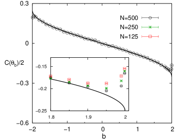
Figure 1: Comparison between the analytical result (solid line) for the $O(1/N)$ coefficient of eq. (40) with numerical diagonalisation of $N\times N$ random matrices drawn from the GOE ensemble. The inset shows the behaviour for different $N$ when the upper band edge is approached.

For $\beta=2$ (GUE), the $O(1/N)$ correction in eq. (40) is zero. This is in contrast to the exact expression for $\rho_{1}(\lambda)$ obtained through supersymmetry [30], replicas [31] and the large $N$ expansion of orthogonal polynomials [31]. These methods show that $\rho_{1}(\lambda)$ is an oscillatory function of $\lambda$ with $N$ maxima. For large but finite $N$, the integration of $\rho_{1}(\lambda)$ over an interval within the support of the spectral density yields a negligible contribution to the $O(1/N)$ correction of $\frac{\left\langle I_{N}\right\rangle}{N}$. This has been confirmed by computing $\left\langle I_{N}\right\rangle/N$ through numerical diagonalisation and then subtracting the leading term of eq. (40), which yields an outcome orders of magnitude smaller than $1/N$. The present approach is not able to recover the correct $O(1/N)$ contribution to $\left\langle I_{N}\right\rangle/N$ due to our replica symmetric assumption for the order parameter. This is evident from the calculation of the spectral density using the fermionic replica method [31], in which the oscillatory correction $\rho_{1}(\lambda)$ is derived by including saddle-points that break replica symmetry.

Let us derive an expression for the variance of the index. Inserting the above expressions for $\Delta_{a}$ and $\Delta_{b}$ in eq. (35) and performing the sum of the convergent series, we can write the formal expression

$$\left\langle I_{N}^{2}\right\rangle-\left\langle I_{N}\right\rangle^{2}=\frac{1}{\beta\pi^{2}}\left[\sum_{\ell=1}^{\infty}\frac{1}{\ell}+\frac{1}{2}\ln{\left(2+2\cos{(2\theta_{b})}\right)}\right]\,.$$ (42)

We have isolated in eq. (42) the divergent contribution to the variance in the form of the harmonic series. This is not surprising, since the leading term of $\left\langle I_{N}^{2}\right\rangle-\left\langle I_{N}\right\rangle^{2}$ should indeed diverge for $N\rightarrow\infty$. The question here is how $\left\langle I_{N}^{2}\right\rangle-\left\langle I_{N}\right\rangle^{2}$ scales with $N$. In order to extract this behaviour in the replica framework, the authors of [3] keep the regularizer $\eta$ finite until the end of the calculation, and then assume there is a functional relation between $\eta$ and $N$. Here a different strategy has been pursued, where the limit $\eta\rightarrow 0^{+}$ has been performed before considering the convergence of the series in eqs. (4) and (35). This approach gives rise to the divergent contribution in eq. (42), which is naturally interpreted as the leading term $\lim_{N\rightarrow\infty}\left\langle I_{N}^{2}\right\rangle-\left\langle I_{N}\right\rangle^{2}$. Thus, in order to understand how the variance scales with $N$, we have to study how the harmonic series diverges. For large $N$, the partial summation behaves as

$$\sum_{\ell=1}^{N}\frac{1}{\ell}=\ln N+\gamma+O(1/N)\,,$$ (43)

where $\gamma$ is the Euler-Mascheroni constant. Consequently, we conclude that the variance behaves for $N\gg 1$ as follows

$$\left\langle I_{N}^{2}\right\rangle-\left\langle I_{N}\right\rangle^{2}=\frac{1}{\beta\pi^{2}}\left[\ln N+\gamma+\frac{1}{2}\ln{\left(2+2\cos{(2\theta_{b})}\right)}\right]\,.$$ (44)

The above equation recovers exactly the leading behaviour of the index variance for $N\gg 1$ [11, 12, 14, 13]. However, eq. (44) fails in reproducing the $O(1)$ correction to $\left\langle I_{N}^{2}\right\rangle-\left\langle I_{N}\right\rangle^{2}$. For $b=0$ and $\beta=2$, the $O(1)$ term in eq. (44) is given by $(\gamma+\ln 2)/2\pi^{2}$, which is only part of the exact result for the GUE ensemble [12]. For $\beta=1$, the $O(1)$ term of eq. (44) does not agree as well with the available result of [3], obtained from a fitting of numerical diagonalisation results. As we shall discuss below, this inaccuracy comes from the replica-symmetric assumption for the order-parameter.

5.2 The number of eigenvalues in a symmetric interval

For the second observable we set $a=-L$ and $b=L$, with $0<L<2$. In this case the random variable $I_{N}$ quantifies the number of eigenvalues within $[-L,L]$. The solutions for $\Delta_{a}$ and $\Delta_{b}$ in the limit $\eta\rightarrow 0^{+}$ read

$$\Delta_{a}=\Delta_{b}^{*},$$ (45)

$$\Delta_{b}=e^{i\theta_{L}},\quad\theta_{L}={\rm arctan}\left(\frac{L}{\sqrt{4-L^{2}}}\right).$$ (46)

Inserting the above forms in eq. (4) and summing the series we obtain

$$\frac{\left\langle I_{N}\right\rangle}{N}=\frac{1}{\pi}\sin{(2\theta_{L})}+\frac{2}{\pi}\theta_{L}+\frac{(2-\beta)}{N}C(\theta_{L}),$$ (47)

with $C(\theta_{L})$ defined in eq. (41).

The leading term $\lim_{N\rightarrow\infty}\frac{\left\langle I_{N}\right\rangle}{N}$ of eq. (47) agrees with the exact result [6]. For $\beta=2$, the $O(1/N)$ correction in the above equation is absent, due to the replica symmetric ansatz for the order parameter. The $O(1/N)$ contribution to $\frac{\left\langle I_{N}\right\rangle}{N}$ can be derived by integrating the $O(1/N)$ correction to the spectral density over $[-L,L]$. In the replica framework, the latter quantity is exactly calculated only when replica symmetry breaking is taken into account [31], i.e., the situation here is completely analogous to the case of the index discussed above. For $\beta=1$, our result for the $O(1/N)$ correction in eq. (47) can be derived from references [27, 28, 29, 30], where the $O(1/N)$ contribution to the spectral density is computed exactly using replicas [27, 28, 29] and supersymmetry [30]. In figure 2 we compare the analytical behaviour of $C(\theta_{L})$ with numerical diagonalisation of real symmetric matrices drawn from the GOE ensemble. Similarly to the $O(1/N)$ correction to the average index, figure 2 illustrates the convergence of the numerical diagonalisation results to the analytical formula of $C(\theta_{L})$ for increasing $N$. However, the variance of $I_{N}$ for Gaussian random matrices displays an abrupt change of behaviour as we reach the scaling regime $2-L=O(N^{-2/3})$ [6, 7], which indicates that our formula for the $O(1/N)$ coefficient might in fact breakdown sufficiently close to $L=2$. A detailed analysis of the behaviour close to the band edges will not be pursued here.

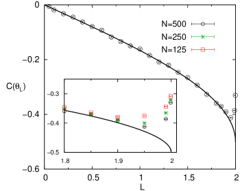
Figure 2: Comparison between the analytical result (solid line) for the $O(1/N)$ term of eq. (47) with numerical diagonalisation of $N\times N$ random matrices drawn from the GOE ensemble. The inset shows the behaviour for different $N$ when the upper band edge is approached.

The variance of the number of eigenvalues $I_{N}$ within $[-L,L]$ is the so-called number variance [1]. The substitution of eqs. (45) and (46) in eq. (35) reads

$$\left\langle I_{N}^{2}\right\rangle-\left\langle I_{N}\right\rangle^{2}=\frac{2}{\beta\pi^{2}}\left[\sum_{\ell=1}^{\infty}\frac{1}{\ell}+\frac{1}{2}\ln{\left(\sin^{2}{(2\theta_{L})}\right)}\right],$$ (48)

where the divergent contribution appears once more as a harmonic series. Following the reasoning of the previous subsection, we conclude that the number variance for $N\gg 1$ is given by

$$\left\langle I_{N}^{2}\right\rangle-\left\langle I_{N}\right\rangle^{2}=\frac{2}{\beta\pi^{2}}\left[\ln N+\gamma+\ln{\left(\sin{(2\theta_{L})}\right)}\right].$$ (49)

The leading contribution for $N\gg 1$ in the above equation is the same as in previous works [6, 7], as long as $L$ is not too close to the band edge $L=2$ [6, 7].

Recently, the replica method has been used to compute the number variance for the Anderson model on a regular random graph [8, 9]. The variance $\left\langle I_{N}^{2}\right\rangle-\left\langle I_{N}\right\rangle^{2}$, when calculated in the microscopic scale $L=O(1/N)$, allows to clearly distinguish between extended, localised and multifractal eigenfunctions [32, 33]. One of the central arguments in [9] is that the limit $\lim_{L\rightarrow 0^{+}}\left\langle I_{N}^{2}\right\rangle-\left\langle I_{N}\right\rangle^{2}$ should give the leading behaviour of the number variance in the relevant regime $L=O(1/N)$. Equation (49) is strictly valid for $L=O(1)$, independently of $N$, but here we can check explicitly this argument by taking the limit $L\rightarrow 0^{+}$ in eq. (49) and then comparing the outcome with standard random matrix results [1]. In the regime where $L\rightarrow 0^{+}$ with $L\gg 1/N$, eq. (49) becomes

$$\left\langle I_{N}^{2}\right\rangle-\left\langle I_{N}\right\rangle^{2}=\frac{2}{\beta\pi^{2}}\left(\ln{s}+\gamma\right),$$ (50)

where $s\equiv LN\gg 1$. The leading term of eq. (50) is in perfect agreement with the standard results for the GOE and the GUE ensembles [1], which supports the essential claim of [9].

5.3 The number of eigenvalues in an arbitrary interval

Lastly, let us present analytical results when $|a|<2$ and $|b|<2$, with $b>a$. In this situation, $\Delta_{a}$ and $\Delta_{b}$ are given by

$$\Delta_{a} = e^{i\theta_{a}},$$

$$\Delta_{b} = e^{i\theta_{b}},$$

where

$$\theta_{a}={\rm arctan}\left(\frac{a}{\sqrt{4-a^{2}}}\right),\qquad\theta_{b}={\rm arctan}\left(\frac{b}{\sqrt{4-b^{2}}}\right).$$ (51)

Inserting the above expressions for $\Delta_{a}$ and $\Delta_{b}$ in eqs. (4) and (35), we obtain

$$\frac{\left\langle I_{N}\right\rangle}{N} = \frac{1}{2\pi}\left[\sin{\left(2\theta_{b}\right)}-\sin{\left(2\theta_{a}\right)}\right]+\frac{1}{\pi}\left(\theta_{b}-\theta_{a}\right)+\frac{(2-\beta)}{2N}\left[C(\theta_{b})-C(\theta_{a})\right],$$

$$\left\langle I_{N}^{2}\right\rangle - \left\langle I_{N}\right\rangle^{2}=\frac{2}{\beta\pi^{2}}\Bigg{\{}\ln N+\gamma+\frac{1}{4}\ln{\left(2+2\cos(2\theta_{a})\right)}+\frac{1}{4}\ln{\left(2+2\cos(2\theta_{b})\right)}$$ (52)

$$- \frac{1}{2}\ln{\left[\frac{1+\cos{\left(\theta_{a}+\theta_{b}\right)}}{1-\cos{\left(\theta_{a}-\theta_{b}\right)}}\right]}\Bigg{\}},$$

in which we have followed a similar calculation as in the previous subsections. We conclude that the leading behaviour of $\left\langle I_{N}^{2}\right\rangle-\left\langle I_{N}\right\rangle^{2}$ for $N\gg 1$ is independent of the interval $[a,b]$. By setting $a=\lambda-L$ and $b=\lambda+L$ in eq. (52), with arbitrary $|\lambda|<2$, the leading term of eq. (52) converges, in the limit $L\rightarrow 0^{+}$, to the leading contribution of eq. (50). Therefore, eq. (50) is not restricted to an interval of size $O(1/N)$ around the center of the band $\lambda=0$, but it holds for any $-2<\lambda<2$, provided $\lambda$ is not too close to one of the band edges.

6 Final remarks

In this work we have applied the replica approach to derive analytical expressions for the mean and the variance of the number $I_{N}$ of eigenvalues within a certain interval of the real line in the case of $N\times N$ Gaussian random matrices. Although the present method has been discussed in previous works for sparse random matrices [18, 8], here we go one step further and explain how the fluctuations of $I_{N}$ for Gaussian random matrices are recovered if one takes into account the $O(1/\sqrt{N})$ correction to the order-parameter around its $N\rightarrow\infty$ limit. Thus, in this work we have not derived novel analytical results, but we have carefully assessed the exactness of the replica-symmetric method by considering random-matrix ensembles for which many exact analytical results are available.

The universal logarithmic scaling $\langle I_{N}^{2}\rangle-\langle I_{N}\rangle^{2}=O(\ln N)$ ($N\gg 1$) of Gaussian random matrices is naturally recovered by studying how the harmonic series diverges. In the limit $L\rightarrow 0^{+}$, eq. (49) for the number variance converges to standard results in the regime $L=O(1/N)$ [1], i.e., when the size of the interval $[-L,L]$ is measured in units of the mean level spacing. This strongly suggests that the present method can be used to inspect the spectral fluctuations at a local scale and, consequently, study the ergodicity of the eigenfunctions, a point raised in a previous work [9].

The reason why our method does not reproduce exactly the $O(1)$ term of $\langle I_{N}^{2}\rangle-\langle I_{N}\rangle^{2}$ lies in the replica-symmetric form of the order-parameter. The variance of $I_{N}$ is directly related to the two-point correlation function $R(\lambda,\lambda^{\prime})=\langle\rho_{N}(\lambda)\rho_{N}(\lambda^{\prime})\rangle$ [33], with $\rho_{N}(\lambda)=N^{-1}\sum_{\alpha=1}^{N}\delta(\lambda-\lambda_{\alpha})$. In the fermionic replica method [31], the replica-symmetric saddle-point yields $R(\lambda,\lambda^{\prime})\propto\left[N\left(\lambda-\lambda^{\prime}\right)\right]^{-2}$ in the regime $|\lambda-\lambda^{\prime}|=O(1/N)$, which gives rise to the leading term of $\langle I_{N}^{2}\rangle-\langle I_{N}\rangle^{2}$. However, the correct $O(1)$ contribution to $\langle I_{N}^{2}\rangle-\langle I_{N}\rangle^{2}$ is only obtained when one includes the oscillatory part of $R(\lambda,\lambda^{\prime})$ [1], which has been exactly derived using both orthogonal polynomials [1] and the supersymmetric approach [34]. In the fermionic replica method, this oscillatory contribution is obtained only by taking into account saddle-points that break replica-symmetry [31].

The present approach also yields an analytical expression for the $O(1/N)$ correction to the average $\left\langle I_{N}\right\rangle/N$, which agrees with exact results in the case of the GOE ensemble [27, 28, 29, 30]. In the case of the GUE ensemble, the replica-symmetric saddle-point is not sufficient to recover the $O(1/N)$ correction to the average $\left\langle I_{N}\right\rangle/N$. This contribution arises from the integration of the $O(1/N)$ oscillatory correction to the average spectral density, which can be only computed by considering replica symmetry breaking [31].

In comparison with the Coulomb gas method [10], whose application is limited to rotationally invariant ensembles, the replica method is more versatile, in the sense it can be applied to random matrix ensembles where the joint distribution of eigenvalues is not analytically known. The present paper opens the door to study the typical eigenvalue fluctuations of a class of random matrix ensembles where, similarly to rotationally invariant random matrices, the eigenvalues strongly repel each other, but their joint distribution is not available. An important example of this class of models is the ensemble of random regular graphs [35, 36], whose fluctuations of $I_{N}$ we will consider in a future work. In addition, it would be interesting to extend the present formalism to include replica symmetry breaking and then compare with the exact results. We leave this matter for future investigation.

References

References

• [1] M. Mehta, Random Matrices. Pure and Applied Mathematics, Elsevier Science, 2004.
• [2] G. Akemann, J. Baik, and P. Di Francesco, The Oxford Handbook of Random Matrix Theory. Oxford Handbooks in Mathematics, OUP Oxford, 2011.
• [3] A. Cavagna, J. P. Garrahan, and I. Giardina, “Index distribution of random matrices with an application to disordered systems,” Phys. Rev. B, vol. 61, pp. 3960–3970, Feb 2000.
• [4] D. Wales, Energy Landscapes: Applications to Clusters, Biomolecules and Glasses. Cambridge Molecular Science, Cambridge University Press, 2003.
• [5] F. J. Dyson, “Statistical theory of the energy levels of complex systems. ii,” Journal of Mathematical Physics, vol. 3, no. 1, pp. 157–165, 1962.
• [6] R. Marino, S. N. Majumdar, G. Schehr, and P. Vivo, “Phase transitions and edge scaling of number variance in gaussian random matrices,” Phys. Rev. Lett., vol. 112, p. 254101, Jun 2014.
• [7] R. Marino, S. N. Majumdar, G. Schehr, and P. Vivo, “Number statistics for $\beta$-ensembles of random matrices: applications to trapped fermions at zero temperature,” ArXiv e-prints, Jan. 2016.
• [8] F. L. Metz and I. Pérez Castillo, “Large deviation function for the number of eigenvalues of sparse random graphs inside an interval,” Phys. Rev. Lett., vol. 117, p. 104101, Sep 2016.
• [9] F. L. Metz and I. Pérez Castillo, “Level compressibility for the Anderson model on regular random graphs and the absence of non-ergodic extended eigenfunctions,” ArXiv e-prints, Mar. 2017.
• [10] F. J. Dyson, “Statistical theory of the energy levels of complex systems. i,” Journal of Mathematical Physics, vol. 3, no. 1, pp. 140–156, 1962.
• [11] S. N. Majumdar, C. Nadal, A. Scardicchio, and P. Vivo, “Index distribution of gaussian random matrices,” Phys. Rev. Lett., vol. 103, p. 220603, Nov 2009.
• [12] S. N. Majumdar, C. Nadal, A. Scardicchio, and P. Vivo, “How many eigenvalues of a gaussian random matrix are positive?,” Phys. Rev. E, vol. 83, p. 041105, Apr 2011.
• [13] I. P. Castillo, “Spectral order statistics of gaussian random matrices: Large deviations for trapped fermions and associated phase transitions,” Phys. Rev. E, vol. 90, p. 040102, Oct 2014.
• [14] I. P. Castillo, “Large deviations of the shifted index number in the gaussian ensemble,” Journal of Statistical Mechanics: Theory and Experiment, vol. 2016, no. 6, p. 063207, 2016.
• [15] S. N. Majumdar and P. Vivo, “Number of relevant directions in principal component analysis and wishart random matrices,” Phys. Rev. Lett., vol. 108, p. 200601, May 2012.
• [16] A. Camacho Melo and I. Pérez Castillo, “A unified approach for large deviations of bulk and extreme eigenvalues of the Wishart ensemble,” ArXiv e-prints, Oct. 2015.
• [17] R. Marino, S. N. Majumdar, G. Schehr, and P. Vivo, “Index distribution of cauchy random matrices,” Journal of Physics A: Mathematical and Theoretical, vol. 47, no. 5, p. 055001, 2014.
• [18] F. L. Metz and D. A. Stariolo, “Index statistical properties of sparse random graphs,” Phys. Rev. E, vol. 92, p. 042153, Oct 2015.
• [19] F. L. Metz, G. Parisi, and L. Leuzzi, “Finite-size corrections to the spectrum of regular random graphs: An analytical solution,” Phys. Rev. E, vol. 90, p. 052109, Nov 2014.
• [20] E. Brézin and S. Hikami, “Characteristic polynomials of random matrices,” Communications in Mathematical Physics, vol. 214, pp. 111–135, Oct 2000.
• [21] E. Brézin and S. Hikami, “Characteristic polynomials of random matrices at edge singularities,” Phys. Rev. E, vol. 62, pp. 3558–3567, Sep 2000.
• [22] A. Borodin and E. Strahov, “Averages of characteristic polynomials in random matrix theory,” Comm. Pure Appl. Math., vol. 59, p. 161, 2006.
• [23] J. P. Keating, Random matrices and the Riemann zeta-function - a review, pp. 210–225. SIAM, 2004.
• [24] M. Mezard, G. Parisi, and M. Virasoro, Spin Glass Theory and Beyond. Lecture Notes in Physics Series, World Scientific, 1987.
• [25] J. Negele and H. Orland, Quantum many-particle systems. Frontiers in physics, Addison-Wesley Pub. Co., 1988.
• [26] R. Kühn, “Spectra of sparse random matrices,” Journal of Physics A: Mathematical and Theoretical, vol. 41, no. 29, p. 295002, 2008.
• [27] J. Verbaarschot and M. Zirnbauer, “Replica variables, loop expansion, and spectral rigidity of random-matrix ensembles,” Annals of Physics, vol. 158, no. 1, pp. 78 – 119, 1984.
• [28] G. S. Dhesi and R. C. Jones, “Asymptotic corrections to the wigner semicircular eigenvalue spectrum of a large real symmetric random matrix using the replica method,” Journal of Physics A: Mathematical and General, vol. 23, no. 23, p. 5577, 1990.
• [29] C. Itoi, H. Mukaida, and Y. Sakamoto, “Replica method for wide correlators in gaussian orthogonal, unitary and symplectic random matrix ensembles,” Journal of Physics A: Mathematical and General, vol. 30, no. 16, p. 5709, 1997.
• [30] F. Kalisch and D. Braak, “Exact density of states for finite gaussian random matrix ensembles via supersymmetry,” Journal of Physics A: Mathematical and General, vol. 35, no. 47, p. 9957, 2002.
• [31] A. Kamenev and M. Mézard, “Wigner-dyson statistics from the replica method,” Journal of Physics A: Mathematical and General, vol. 32, no. 24, p. 4373, 1999.
• [32] S. A. K. B. L. Altshuler, I. K. Zharekeshev and B. I. Shklovskii, “Repulsion between energy levels and the metal-insulator transition,” J. Exp. Theor. Phys., vol. 67, p. 625, 1988.
• [33] A. D. Mirlin, “Statistics of energy levels and eigenfunctions in disordered systems,” Physics Reports, vol. 326, no. 5–6, pp. 259 – 382, 2000.
• [34] K. B. Efetov, “Supersymmetry and theory of disordered metals,” Adv. Phys., vol. 32, pp. 53–127, 1983.
• [35] N. C. Wormald, “Models of random regular graphs,” in Surveys in Combinatorics, pp. 239–298, University Press, 1999.
• [36] B. Bollobás, Random Graphs. Cambridge University Press, second ed., 2001. Cambridge Books Online.