mixing in the Khuri-Treiman equations for
Abstract:
A reliable determination of the isospin breaking double quark mass ratio from precise experimental data on decays should be based on the chiral expansion of the amplitude supplemented with a Khuri-Treiman type dispersive treatment of the final-state interactions. We discuss an extension of this formalism which allows to estimate the effects of the and resonances and their mixing on the amplitudes. Matrix generalisations of the equations describing elastic rescattering with are introduced which accomodate both and coupled-channel rescattering. Isospin violation induced by the physical mass difference and by direct mass difference effects are both accounted for in the dispersive integrals. Numerical solutions are constructed which illustrate how the large resonance effects at 1 GeV propagate down to low energies. They remain small in the physical region of the decay, due to the matching constraints with the NLO chiral amplitude, but they are not negligible and go in the sense of further improving the agreement with experiment for the Dalitz plot parameters.
1 Introduction
Precise measurements of Dalitz plot distributions of the (see [1]) and decays (see [2]) have been performed recently (see also the talks by S. Giovannella and S. Fang at this conference). These measurements provide precious insights into the workings of the chiral expansion beyond the next-to-leading order (NLO) which is necessary in order to arrive at a reliable and precise determination of the isospin breaking double quark mass ratio
| (1) |
As an illustration of the importance of NNLO effects, consider the slope parameter in the Dalitz plot. The NLO prediction [3] depends on no coupling constant (except ) but fails to agree with experiment,
| (2) |
The calculation of the amplitudes at NNLO has been performed [4] but, in this case, predictivity is limited by the absence of model independent determination of the relevant coupling constants .
Part of the (and higher order) chiral effects can be attributed to final-state interactions (FSI). Indeed, the chiral NLO amplitude accounts for the FSI at only. The attractive idea was proposed long ago to treat the FSI part exactly through dispersive methods while using the chiral expansion in unphysical sub-threshold regions [5, 6, 7, 8] and then match the two representations. The formalism proposed by Khuri and Treiman [9] for treating the -wave FSI in three-body decays was extended to -wave rescattering and applied to the amplitude in refs. [7, 8]. Here, we investigate a further extension of the KT equations, which goes beyond the elastic approximation, and thereby includes the influence of the resonant mixing effects. In this regard, the formalism accounts for isospin breaking induced by the mass difference via unitarity, first considered in ref. [10], as well as the direct quark mass matrix effects.
2 Khuri-Treiman formalism with chiral NLO matching: elastic case
Khuri and Treiman [9] have shown that the final-state interaction problem, for three-body decays, can be recast as a problem of solving sets of integral equations involving functions of one variable. Its application to the amplitudes [7, 8] involves three functions, , such that the charged decay amplitude can be expressed as follows,
| (3) |
and
| (4) |
The Mandelstam variables are given by , , . Under the assumption of elastic unitarity, the equations can be expressed in terms of the Omnès functions,
| (5) |
where is the elastic phase shift with isospin and or . The KT equations, in the four-parameter version proposed in ref. [8], have the following form
| (6) |
where
| (7) |
(with when and when ). The functions , finally, are the left-cut parts of the partial-wave amplitudes with ,
| (8) |
with . The functions can be expressed in terms of the functions via the representation (3) and performing partial-wave projections, such that the equations (6) form a linear, self-consistent system. It is easy to verify that these equations ensure that the partial-wave amplitudes satisfy the correct elastic unitarity equations,
| (9) |
Strictly speaking, this form is valid in the unphysical situation where . The analytical continuation of eq. (9) to the physical case is performed by replacing the imaginary part by the discontinuity across the unitarity cut (divided by ). Furthermore, in that case, the complex cut of the functions overlaps with the unitarity cut and these functions diverge at the pseudo-threshold . The integrals can also be defined (and are finite) by analytic continuation. All these subtle points are explained in detail in ref. [7].
Clearly, the representation (3) is not the most general one for an amplitude which depends on two independent variables and must therefore hold only in a restricted region of the Mandelstam variables. It is also easy to check that this representation implies
| (10) |
which cannot be exactly correct but represents an acceptable approximation when the corresponding phase-shifts are small, that is, in the region .
2.1 Matching conditions
The parameters , , , originate from the presence of subtractions in the dispersive representations of the functions . These are necessary in order to reduce the dependence on the integration region . We consider here a version which leads to four polynomial parameters. It is particularly convenient, since, in this case, all the parameters can be fixed from matching with the NLO chiral amplitude. The matching conditions are obtained from the simple requirement that the difference between the dispersive and the chiral amplitude of order should be of chiral order , i.e., in our case,
| (11) |
This relation is satisfied automatically for the imaginary part of the difference, which implies that the real part can be expanded as a polynomial as a function of the variables , , . Equating this polynomial to zero gives four independent equations. Expressing the chiral amplitude in the same form as eq. (3) in terms of three functions (see [8]) these four matching equations can be written as follows,
| (12) |
where all functions and their derivatives are to be taken at . Note that the integrals carry a linear dependence on the four polynomial parameters.
3 KT equations for with inelastic channels
3.1 Difficulties of the general extension
The assumption of elastic unitarity seems well justified for since the energy and elastic unitarity is known to hold to a good approximation in the region GeV. However, the KT equations involve integrals over an infinite energy range. In the Omnès integrals, for instance, there is an arbitrariness as to the choice of the phase to be used above the threshold. The subtractions and the matching equations ensure that the dispersive amplitude in the low energy region should not depend too much on the choice of phase above 1 GeV. Nevertheless, having a small number of subtractions, one expects that an improved treatment of the 1 GeV region, should result in better precision at low energy. At 1 GeV, the two resonances and are present and a sharp onset of inelastic scattering in the -wave is observed.
Extending the unitarity relations to include the three channels leads one to consider the transition amplitudes from , , to , , and to , . Each of these physical amplitudes can be expressed in terms of functions of one variable, analogous to eq. (3). Unfortunately, a separation of each amplitude into an isospin violating and an isospin conserving component is not possible at this level because the kinematical constraint on is different for and amplitudes. This separation can be made only after performing the partial wave projections. This feature complicates the derivation of a general self-consistent set of KT equations including the channels. In the following, we will show that a simple approximation can be made which should provide a sensible order of magnitude for the influence of these channels on the amplitude.
3.2 Coupled-channel unitarity relations
Let us now focus on the partial waves. We will have to consider the following isospin conserving amplitudes with
| (13) |
while for , coupling to cannot occur and we will continue to use the elastic approximation in that case111Inelasticity will also be ignored for scattering. Recall that we are mainly interested here in accounting for the effects of the scalar resonances.. We can classify the isospin violating amplitudes into two classes: a) transitions and b) transitions,
| (14) |
We can then write the unitarity relations for these two sets of isospin violating amplitudes which now include inelasticity. For , and to first order in isospin breaking, they read
| (15) |
with
| (16) |
and
| (17) |
The last term in eq. (15) accounts for isospin violation induced by the mass difference via the function
| (18) |
The unitarity relation for the amplitudes, now, reads
| (19) |
3.3 Coupled-channel KT equations
The next step is to separate each isospin violating partial-wave amplitude, which is an analytic function with two cuts into two functions, one having a right-hand cut and one having a left-hand cut. In matrix form,
| (20) |
It is now easy to derive a matrix generalisation of the KT equations (6) involving and . For the matrix , one has
| (21) |
where are Muskhelishvili-Omnès (MO) matrices, which must be computed numerically from the -matrices and is a matrix of polynomials involving 12 parameters. The matrices of integrals, finally, read
| (22) |
and
| (23) |
they correspond to the two different types of contributions in the unitarity relation for . Note that in the integrals isospin violation is induced by the physical mass difference. As in the one channel case, the representation (21) ensure that the unitarity relations (15) for are satisfied. It also ensures that each component in the matrix satisfies a twice-subtracted dispersion relation associated with its right-hand cut,
| (24) |
Verifying that eq. (24) is satisfied is a good check of the numerical implementation of the KT representation (21).
3.4 Matching equations
For the amplitudes we can use, as before, the four matching equations associated with the NLO chiral amplitudes. The set of matching equations (12) is easily generalised to the coupled-channel situation by using the corresponding KT representations for , , . In contrast, for the amplitudes which involve the channels, we do not have a complete set of self-consistent KT equations which would enable us to determine the left-cut functions in terms of the right-cut ones. Thus, we cannot use the NLO amplitudes to perform the matching. The set of equations is sufficient, however, for matching to leading order chiral amplitudes. Indeed, at LO the chiral amplitudes have no left-hand cut. Accordingly, we can make the approximation to set the left-cut functions equal to zero when and . The polynomial parameters may then be fixed such as to reproduce the expressions
| (27) |
The low energy behaviour of the these isospin violating amplitudes, resulting from this matching procedure, is illustrated on fig. 1.


4 Some results and comparisons with experiment
4.1 Muskhelishvili-Omnès matrices ,
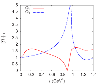
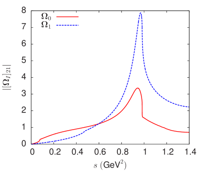
We still need to define the MO matrices which enter in the formulation of the coupled-channel KT equations (21) (25). For , we can rely on extensive phase-shift analysis of scattering performed long ago. New high-precision measurements of the -wave phase shift near threshold from decays have appeared [11] and new Roy equations solutions have been derived [12, 13]. Measurements of the inelastic amplitude have also been performed (see e.g. [14]). This allows one to derive a two-channel model for the -matrix and then, imposing appropriate asymptotic conditions, to compute numerically the corresponding MO matrix by standard methods [15, 16]. For , in contrast, there have been no measurements of scattering phase-shifts, but the properties of the have been established via its final-state interaction effects. We will use here a two-channel -matrix model [17] constrained by the properties of the and resonances and by matching with NLO ChPT at low energy. We also used implemented NLO chiral results on and form factors, which are linearly related to the MO matrix , and provide additional constraints on the behaviour of the phase shifts above 1 GeV. As an illustration, we show in fig. 2 the modulus of the components , for .
4.2 amplitudes from KT solutions
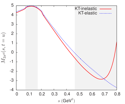
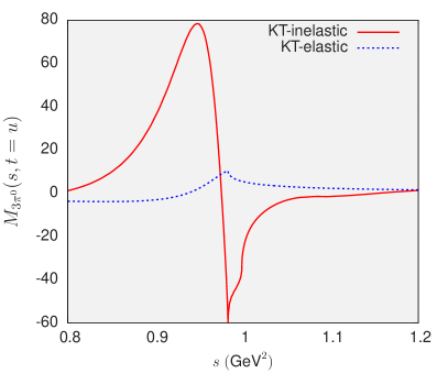
Results for the amplitude obtained from solving the KT equations in the elastic approximation and their inelastic extension as discussed above, are shown in fig. 3. The figure shows that the and resonances induce a very large energy variation in the 1 GeV region, which is essentially absent in the elastic approximation, and how this effect propagates down to lower energies.
Numerical (preliminary) results for the Dalitz plot parameters of and are shown in table 1 and compared with experimental results. The results associated with KT solutions are predictions based on the matching equations (12) and involve no fitted parameter. The improvement, as compared to using the chiral NLO amplitude directly in the physical region is spectacular222We agree on this point with the results of ref. [7] but not with [18] who made some approximations when implementing the matching conditions.. The effects of the resonances can be as large as 10% and seem to improve the agreement with experiment, in particular for the parameter .
5 Conclusions
We have developed a formalism which, within a simple approximation scheme, allows us to take into account the influence of the scalar resonances , as well as the mass difference in the amplitude within the dispersive framework of Khuri and Treiman. Matching with the chiral amplitude in the sub-threshold region, a prediction for the Dalitz plot parameters is achieved which agrees reasonably well with experiment and this agreement is improved when the scalar resonances are introduced. These results suggest that residual effects (i.e. which cannot be ascribed to final-state interactions) could be relatively small. An estimate of these effects should, however, be useful for deriving a precise value of the double quark mass ratio Q.
Param.
KT-elastic
KT-coupled
WASA
KLOE
a
-1.320
-1.154
-1.146
-1.144(18)
-1.090(14)
b
0.422
0.202
0.181
0.219(19)
0.124(11)
f
0.015
0.107
0.116
0.115(37)
0.140(20)
d
0.083
0.088
0.090
0.086(18)
0.057(17)
Param.
KT-elastic
KT-coupled
PDG
+0.014
-0.027
-0.031
-0.0315(15)
Acknowledgments.
This research was supported by Spanish Ministerio de Economía y Competitividad and European FEDER funds under contracts FIS2014-51948-C2-1-P, FPA2013-40483-P and FIS2014-57026-REDT, and by the European Community-Research Infrastructure Integrating Activity ”Study of Strongly Integrating Matter” (acronym HadronPhysics3, Grant Agreement Nr 283286) under the Seventh Framework Programme of the EU. M. A. acknowledges financial support from the ”Juan de la Cierva” program (reference 27-13-463B-731) from the Spanish Government through the Ministerio de Economía y Competitividad.References
- [1] F. Ambrosino et al. (KLOE), JHEP 0805, 006 (2008), 0801.2642, P. Adlarson et al. (WASA@COSY), Phys.Rev. C90(4), 045207 (2014), 1406.2505
- [2] C. Adolph et al. (WASA@COSY), Phys.Lett. B677, 24 (2009), 0811.2763, M. Unverzagt et al. (Crystal Ball@MAMI , TAPS , A2), Eur.Phys.J. A39, 169 (2009), 0812.3324, S. Prakhov et al. (Crystal Ball@MAMI, A2), Phys.Rev. C79, 035204 (2009), 0812.1999, F. Ambrosino et al. (KLOE), Phys.Lett. B694, 16 (2010), 1004.1319
- [3] J. Gasser, H. Leutwyler, Nucl.Phys. B250, 539 (1985)
- [4] J. Bijnens, K. Ghorbani, JHEP 0711, 030 (2007), 0709.0230
- [5] A. Neveu, J. Scherk, Annals Phys. 57, 39 (1970)
- [6] C. Roiesnel, T.N. Truong, Nucl. Phys. B187, 293 (1981)
- [7] J. Kambor, C. Wiesendanger, D. Wyler, Nucl.Phys. B465, 215 (1996), hep-ph/9509374
- [8] A. Anisovich, H. Leutwyler, Phys.Lett. B375, 335 (1996), hep-ph/9601237
- [9] N. Khuri, S. Treiman, Phys.Rev. 119, 1115 (1960)
- [10] N. Achasov, S. Devyanin, G. Shestakov, Phys.Lett. B88, 367 (1979)
- [11] J. Batley et al. (NA48-2), Eur.Phys.J. C70, 635 (2010)
- [12] B. Ananthanarayan, G. Colangelo, J. Gasser, H. Leutwyler, Phys. Rept. 353, 207 (2001), hep-ph/0005297
- [13] R. Garcia-Martin, R. Kaminski, J.R. Pelaez, J. Ruiz de Elvira, F.J. Yndurain, Phys. Rev. D83, 074004 (2011), 1102.2183
- [14] B.R. Martin, D. Morgan, G. Shaw, Pion Pion Interactions in Particle Physics (Academic press, London, 1976)
- [15] O. Babelon, J.L. Basdevant, D. Caillerie, G. Mennessier, Nucl.Phys. B113, 445 (1976)
- [16] J.F. Donoghue, J. Gasser, H. Leutwyler, Nucl.Phys. B343, 341 (1990)
- [17] M. Albaladejo, B. Moussallam (2015), 1507.04526
- [18] S. Lanz, Ph.D. thesis, University of Bern (2011)