Wave equations on the linear mass Vaidya metric

Abstract

We discuss the near singularity region of the linear mass Vaidya metric. In particular we investigate the structure in the numerical solutions for the scattering of scalar and electromagnetic metric perturbations from the singularity. In addition to directly integrating the full wave-equation, we use the symmetry of the metric to reduce the problem to that of an ODE. We observe that, around the total evaporation point, quasi-normal like oscillations appear, indicating that this may be an interesting model for the description of the end-point of black hole evaporation.

I Introduction

The Vaidya metric is a useful solution to Einstein’s equations with a stress-energy tensor that corresponds to an outgoing, spherically symmetric flux of radiation vaidya . It has been used as a model for the metric outside stars that includes the back-reaction of the space-time to the stars radiation, and also as a model for various studies of both black hole formation and evaporation waugh862 ; bicak97 ; hiscock82 ; kuroda ; balbinot ; abdalla ; bicak03 ; ghosh ; harko ; girotto ; kawai ; fayos10 ; farley . The linear mass Vaidya metric is a special class of Vaidya metrics over which one has a certain degree of analytic control, in particular as a consequence of the additional homothety symmetry that these metric possess. For a restricted range of parameters in the outgoing Vaidya metric with linear mass the metrics contain a null singularity that vanishes at a point internal to the space-time and thus is an ideal exact candidate for a model of a decaying black hole.

In a previous paper OLoughlin:2013aa a particular scenario was introduced and an initial study of the behaviour of metric perturbations was presented in support of this model. The out-going Vaidya metric with monotonically decreasing linear mass function can resemble a realistic situation for the final phase of black hole evaporation. In this paper we study in more detail the electromagnetic and scalar perturbations of the out-going linear mass Vaidya metric in this context, in particular to study the perturbation equations of this dynamical space-time results looking for a quasi-normal (QN) like ringing. Such results would give support to the claim that this metric is black-hole like around the vanishing point of the singularity and thus is suitable to be considered as the transitional state between an adiabatically evaporating Schwarzschild black hole at the end stage of its life and Minkowski space-time.

Quasi-normal modes (QNMs) qnmbs1 ; qnmbs2 for time-dependent backgrounds have been investigated in Hod:2002gb ; Xue:2003vs ; Shao:2004ws and in particular for in-going Vaidya metric in invai1 ; invai2 . The general shape of the oscillations for dynamical backgrounds like Vaidya is different from that of the stationary ones like Schwarzschild. In the stationary adiabatic regime the real part of QNMs changes inversely with the mass function. For dynamical backgrounds where the mass changes with time, the period of the oscillation will also change, thus the shape of the waveform includes oscillations with varying periods. The power law fall off of the tail of QNMs originally calculated by Price price1972 for stationary space-time is also different for dynamical backgrounds Hod:2002gb ; Hod:2009my . Numerical errors in the investigation of tail phenomena in dynamical background are unavoidable so to have a better picture of this phenomena one should also more analytic methodes if they are available.

In this paper we use both numerical and analytical methods to study the response of the out-going Vaidya background to the electromagnetic and scalar perturbation. We first write the perturbation equations in double null coordinates Waugh:1986aa and then we solve the partial differential equations (PDE) numerically. To provide an alternative, more analytic approach we then use the homothety symmetry of the linear mass vaidya metric to reduce the problem to that of an ordinary differential equation and comment on the results.

II Outgoing Vaidya Space-Time

The Vaidya metrics vaidya are exact solutions of the Einstein equations. In radiation coordinates $(w,r,\theta,\phi)$ this metric has the form

$$ds^{2}=-(1-\frac{2m(w)}{r})dw^{2}+2cdwdr+r^{2}d\Omega^{2},$$ (1)

where $c=1,-1$ respectively corresponds to ingoing and outgoing radial flow, $w=t+cr$ and $m(w)$ is a monotonic mass function. In the presence of spherical symmetry this mass function can be the measure of the amount of energy within a sphere with radius $r$ at a time $t$ Zannias:1990aa ; Nielsen:2008kd .

The causal and singularity structure of this space-time can change significantly with the choice for the mass function. For constant mass this solution reduces to the Schwarzschild solution in ingoing or outgoing Eddington-Finkelstein coordinates. The ingoing Vaidya metric describes collapsing null dust Gao:2005yq . The outgoing Vaidya space-time

$$\begin{split}&ds^{2}=-f(u,r)du^{2}-2dudr+r^{2}d\Omega^{2}\\ &f(u,r)=(1-\frac{2m(u)}{r})\end{split}$$ (2)

describes the evolution of a radiating star or black hole, where $m(u)$ is the mass function of retarded time $u$ that labels the outgoing radial null geodesics. In the following we will restrict our analysis to the outgoing case as we are interested in the final stages of black hole evaporation.

The only non-vanishing component of the Einstein tensor is

$$G_{uu}=-(\frac{2}{r^{2}})\frac{dm(u)}{du},$$ (3)

and the stress-energy tensor that leads to this solution is

$$T_{\alpha\beta}=-\frac{1}{4\pi r^{2}}\frac{dm(u)}{du}k_{\alpha}k_{\beta}$$ (4)

where $k_{\alpha}$ is tangent to radial outgoing null geodesic, $k_{\alpha}k^{\alpha}=0$. This stress-energy tensor describes a pressure less fluid with energy density $\rho=-\frac{dm(u)}{du}4\pi r^{2}$ moving with four-velocity $k_{\alpha}=\delta_{\alpha}^{u}$ (such a fluid is called “null dust”). To satisfy the null energy condition for which $\rho\geq 0$, the mass function $m(u)$ must be a decreasing function of increasing retarded time, namely $\frac{dm(u)}{du}<0$, which means that the mass function decreases in response to the outflow of radiation as one would expect for the evolution of a radiating star or an evaporating black hole. For our analysis we will choose the linear mass function $m(u)=-\mu u$. This choice of mass function will enable us to study the possible evolution of the space-time around the end point of black hole evaporation.

In addition to the spherical symmetry of this space-time (2) it is also homothetic in the case that the mass function is linear. The space-time possesses a conformal Killing vector $K$Hiscock:1982pa

$$K_{\mu;\nu}+K_{\nu;\mu}=2\rho g_{\nu\mu}$$ (5)

where $\rho$ is a constant, indicating that this is actually a homothety symmetry. Homothety means that the metric with linear mass function scales upon a scaling of the coordinates by an overall factor

$$(u,r)\rightarrow(\zeta u,\zeta r)\quad\quad\Rightarrow\quad\quad ds^{2}\rightarrow\zeta^{2}ds^{2},$$ (6)

for any real $\zeta$.

II.1 The conformal structure of linear-mass Vaidya space-times

In general the choice of mass function in Vaidya space-time determines its global and local structure and singularities. Here we will consider only the case of a linear mass function $m(u)=-\mu u$ and the conformal structure of the space-time varies with $\mu$ Waugh:1986aa in the following way. For $\mu>1/16$ the conformal diagram is displayed in figure (1).

Figure 1: Conformal diagram for outgoing Vaidya with linear mass function for $\mu>1/16$, dot-dashed line represents $r=0$ singularity.

Figure 2: Conformal diagram for outgoing Vaidya with linear mass function for $\mu=1/16$, dot-dashed lines represent $r=0$ singularities.

Figure 3: Conformal diagram for outgoing Vaidya with linear mass function for $\mu<1/16$, dot-dashed lines represent $r=0$ singularities.

The dot-dashed line shows the singularity at $r=0$ for $u<0$. The next case is $\mu=1/16$ which is represented in figure (2). In the last case in figure (3) the conformal diagram for $\mu<1/16$ is shown. In this case the $u=0$ boundary to the future of the endpoint of the $r=u=0$ singularity is special in that the space-time there approaches that of Minkowski space. Indeed it has been shown in Unruh:1985aa that one can continuously attach the metric along this part of the $u=0$ hypersurface to Minkowski space without introducing curvature singularities.

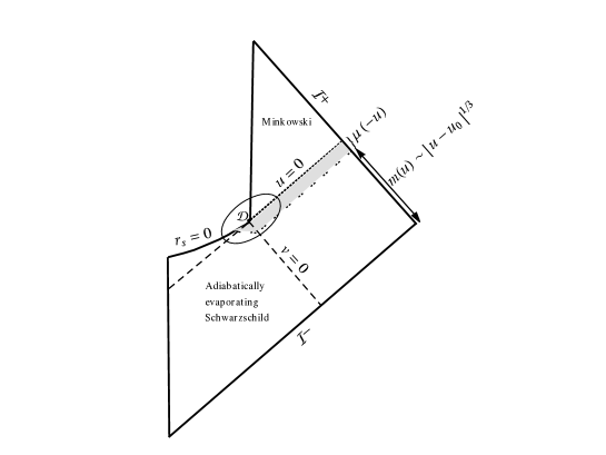
Figure 4: Conformal diagram for the evaporation of a Schwarzschild black hole with linear Vaidya at the final stage of evaporation and a future Minkowski region.

Considering the outgoing Vaidya metric with linear mass function and with $\mu<1/16$, a new model for the final fate of a black hole at the end of its evaporation has been proposed in OLoughlin:2013aa . This space-time can be divided into three different regions characterized by a transition time $u_{t}$ and illustrated in figure 4: an adiabatic Schwarzschild region for all $v$ with $u<u_{t}$ with $m(u)\sim|u-u_{0}|^{1/3}$ and also most of the region $v<0$; a Vaidya region with linear mass function for $u_{t}<u<0$, $v\geq 0$; a Minkowski space-time region for $u>0$, $v>0$. In this model the linear mass function is used when the mass of black hole becomes Planckian.

II.2 Vaidya in Double Null Coordinates

As our purpose is to study wave-equations on the outgoing Vaidya space-time, it is very useful to introduce the double null coordinate Waugh:1986aa for which both semi-analytical and numerical calculations can be performed. In these coordinates $(u,\theta,\phi,v)$ the general form of the metric is

$$ds^{2}=-2f(u,v)dudv+r^{2}(u,v)d\Omega^{2}$$ (7)

For the outgoing metric, the energy momentum tensor has the form

$$T_{\mu\nu}=\frac{\mu}{4\pi r(u,v)^{2}}(\delta_{\mu}^{u})(\delta_{\nu}^{u})$$ (8)

Considering the linear mass function with $\mu<1/16$ and introducing $\Delta=\sqrt{1-16\mu}$, $f(u,v)$ is

$$f(u,v)=\frac{1+\Delta}{2\Delta r(u,v)}(r(u,v)+u(1-\Delta)/4)^{2/(1+\Delta)},$$ (9)

where $r(u,v)$ can be derived by solving this equation

$$\begin{split}&\left(\frac{v}{|u|^{2\Delta/(1+\Delta)}}\right)^{1+\Delta}\left(\frac{r(u,v)}{|u|}-\frac{1-\Delta}{4}\right)^{1-\Delta}\\ &=\left(\frac{r(u,v)}{|u|}-\frac{1+\Delta}{4}\right)^{1+\Delta}.\end{split}$$ (10)

The function $r(u,v)$ can be found exactly for $\Delta=3/5,1/2,1/3,1/5,1/7$ and the explicit solutions have been given in OLoughlin:2013aa .

III Vaidya Potential

In general QNMs are are found as decaying oscillations in the metric perturbation close to the horizon of a black hole. The frequencies of these modes generally have a complex form of which the real part represent the oscillation frequency and the imaginary part represents the damping of the oscillation. QNMs can be calculated for both stationary and time dependent background and they are black holes fingerprints. The evolution of the response of the black hole to perturbations can be divided in three stages: first an initial wave burst in a relatively short time by the source off perturbation, then the “ringing radiation” which is caused by the damped oscillations of QNMs that are excited by the source of perturbation and finally a power law tail suppression of QNMs at very late time due to the scattering of the wave by the effective potential.

In order to study possible QN like modes of Vaidya space-time, we need to study the wave equations for perturbations of the space-time metric ReggeWheeler which are naturally divided into scalar, electromagnetic and tensorial modes,

$$\frac{\partial^{2}\psi}{\partial u\partial v}+W(u,v)f(u,v)\psi=0$$ (11)

where $W(u,v)$ is given by

$$W(u,v)=\frac{\ell(\ell+1)}{2r^{2}(u,v)}+\sigma\frac{m(u)}{r^{3}(u,v)}$$ (12)

and where $\sigma=1$ and $\sigma=0$ correspond, respectively, to the scalar and electromagnetic perturbations on which we will focus the current study. From here on, for calculational convenience, we extend the linear mass function $m(u)=-\mu u$ to all values of $u<0$ and not just for the $u_{t}<u<0$ as was shown in figure (4). Equation (11) describes wave propagation in the Vaidya background and $f(u,v)W(u,v)$ is the effective potential which describes how fields are scattered by the geometry. It is clear that this potential depends on the black hole geometry and also on the spin of the perturbation under consideration.

III.1 Integrating the PDE

We proceed by using the numerical integration technique for the calculation of QNMs originally proposed and developed in Gundlach:1994 . In the present context this equation was already studied for the special case of electromagnetic perturbations with $\ell=1$ in OLoughlin:2013aa where it is was observed that an initially ingoing gaussian wave-packet coming in from ${\mathcal{I}}^{-}$ with centre at small negative $\bar{v}$ appears to develop a QN like ringing as it evolves towards $\bar{u}\to 0$.The numerical integration was carried out by sending in the direction of increasing $u$ a gaussian wave localized around $v_{c}<0$.

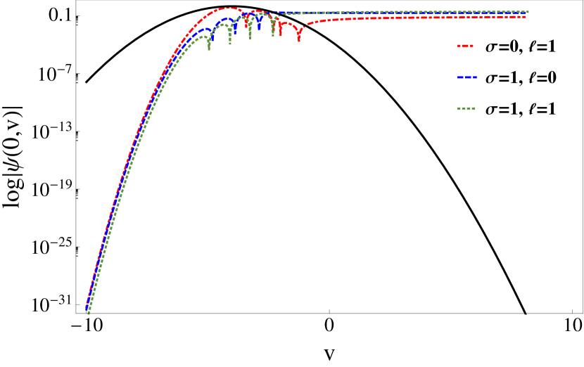
(a) $w=1$, $v_{c}=-4$

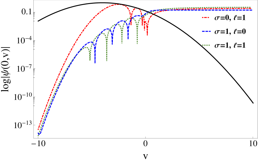
(b) $w=2$, $v_{c}=-4$

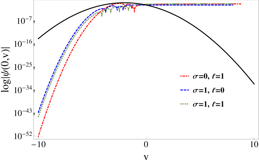
(c) $w=1$, $v_{c}=-2$

Figure 5: Time profile of the response of outgoing Vaidya space-time to the electromagnetic and scalar perturbations for $\Delta=1/2$ and $\ell=0,\ell=1$ for different values of the initial data. The solid curve indicate the Gaussian function that has been used as initial data where $w$ is the width and $v_{c}$ marks the center of the Gaussian.

In this paper, in addition to the calculation for the electromagnetic field we also present the numerical integration to obtain the time profile of the perturbed outgoing Vaidya for both electromagnetic $\sigma=0$ and scalar perturbations $\sigma=1$ and for different angular momentum values. Some selected results for the evolution of the ingoing wave are presented in figure (5). In these figures the results of the integration with $\Delta=1/2$ are displayed. Similar results can also be obtained for other values of $\Delta$. The initial conditions were a gaussian wave form in $v$ with centre at $v=v_{c}$ at $u=u_{0}=-40$ and with varying widths. One can see that in particular there is a ringing of varying period for $\bar{v}\lesssim 0$. The ringing dies out rapidly and is not present for $v>0$ in line with the fact that the “Planckian” black hole has vanished. The general form of these oscillations doesn’t change for different values of the initial gaussian, though their detailed structure does. This indicates that there are not true QNMs at particular discrete frequencies in contrast to what one finds for the Schwarzschild black hole.

These results are in line with earlier studies of QNMs for dynamical backgrounds Xue:2003vs where it was been pointed out that when the black hole mass decreases with time the oscillation period becomes shorter in contrast to the constant frequency QNMs of the Schwarzschild black hole. These solutions show a constant tail after few oscillations for large values of $v>0$ however we will see in the next section that as a consequence of the homothety of the metric and the initial conditions that the $|\psi|\rightarrow\text{const}$ behavior at large positive $v$ is most likely a consequence of numerical errors. In Hod:2002gb ; Hod:2009my has been shown that the there is time window between the dominant period of QN ringing and the tail of these modes. In effect the tail behavior with a pure power law decay is only expected at infinitely late times. In practice the numerical integration is for a finite time interval and this causes an inherent error in the behavior of the tail.

In the next subsection we will show that, as a consequence of the scaling symmetry, the wave-equation can be separated, thus reducing the problem to that of an ordinary differential equation. We will also see from the separation ansatz that evolution is essentially a frequency dependent rescaling of the modes that are used to construct the initial Gaussian profile.

III.2 Reduction to an ODE

The main purpose of the current research was to present the wave-profiles that one can obtain from the numerical mesh integration method for different initial conditions and fields, as carried out in the previous section, and then to compare them with the individual mode solutions that we will obtain below via a semi-analytic method that takes advantage of the scaling symmetry of the space-time and equations. We will now look at individual modes of the wave-function that we obtain by using the homothety symmetry of the equations to carry out a separation of variables in the differential equation (11).

The homothety symmetry of this space-time suggests that we change the variable as follows

$$\bar{u}=-u=|u|,\quad\quad\bar{v}=v(-u)^{-2\Delta/(1+\Delta)},$$ (13)

giving (from (10))

$$r=r(u,v)=|u|g(v/|u|^{2\Delta/(1+\Delta)}).$$ (14)

Applying these changes to equation (11)

together with the ansatz

$$\psi_{\lambda}(\bar{u},\bar{v})=\bar{u}^{\lambda}V_{\lambda}(\bar{v}),$$ (15)

we obtain the following differential equation

$$\bar{v}\frac{\partial^{2}V(\bar{v})}{\partial\bar{v}^{2}}+(1-\kappa)\frac{\partial V(\bar{v})}{\partial\bar{v}}+F(\bar{v})V(\bar{v})=0$$ (16)

where $\kappa=\lambda/\alpha$ with $\alpha=\frac{2\Delta}{(1+\Delta)}$ and

$$\begin{split}F(\bar{v})=&\frac{1}{2\alpha^{2}g(\bar{v})^{4}}\left(g(\bar{v})-\frac{(1-\Delta)}{4}\right)^{2/(1+\Delta)}\\ &(\ell(\ell+1)g(\bar{v})+2\sigma\mu).\end{split}$$ (17)

In figure (6) we have shown the function $F(\bar{v})$ for $\Delta=1/2$.

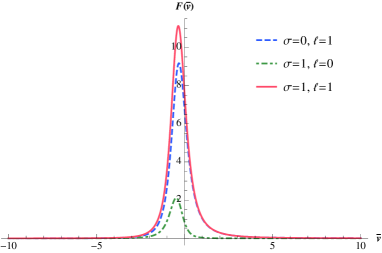
Figure 6: (a) $F(\bar{v})$ for $\Delta=1/2$ and $\sigma=0,1$, for $3$ different values of angular momentum

To obtain some more information about the eigenvalue $\lambda$ we will first consider the behavior of the solutions to (16) around $\bar{v}=0$. Expanding $V(\bar{v})$ around $\bar{v}\to 0$

$$V(\bar{v})=\bar{v}^{s}\sum_{n=0}^{\infty}{a_{n}\bar{v}^{n}}\quad F(\bar{v})=\sum_{n=0}^{\infty}{b_{n}\bar{v}^{n}}$$ (18)

with $b_{0}\neq 0$ we obtain from (16) the indicial equation

$$s(s-\kappa)=0,$$ (19)

which to leading order gives

$$V(\bar{v})=\alpha+\beta\bar{v}^{\kappa}$$ (20)

and thus

$$\psi_{\lambda}=\alpha\bar{u}^{2\kappa/3}+\beta v^{\kappa}.$$ (21)

Decomposing $\kappa=-i\omega+\epsilon$ into real and imaginary parts, we see that well-behaved solutions around $v=0$ require that $\epsilon\geq 0$. Note that this also means that around $v=0$ the $\bar{u}$ dependent term is finite as $\bar{u}\rightarrow 0$, in agreement with the results of the numerical integration presented in the previous section. Obviously this implies a divergence for large $\bar{u}$, but our physical setup does not include this region.

To obtain further information about the global structure of the solutions to the wave-equation we can expand around large positive $\bar{v}$. For large $\bar{v}$ approaching ${\mathcal{I}}_{+}$ we make the substitution $\bar{v}=e^{\bar{x}}$ and to leading order we also have $F(\bar{v})\sim c\leavevmode\nobreak\ \ell(\ell+1)/\bar{v}^{5/2}$, for some constant $c$. Together with the above substitution we obtain the equation

$$\ddot{V}-\kappa\dot{V}+c\leavevmode\nobreak\ \ell(\ell+1)e^{-5\bar{x}/2}=0.$$ (22)

The leading large $\bar{x}$ solution is

$$V(x)=\gamma+\delta e^{\kappa\bar{x}}$$ (23)

leading to (with $v=e^{x}$),

$$\psi_{\lambda}=\gamma\bar{u}^{2\kappa/3}+\delta e^{\kappa x}$$ (24)

and thus one has an outgoing wave of frequency $\omega$ for $\kappa=-i\omega$, requiring again that $\epsilon=0$. Note that the expansion around infinity has the same leading behavior as that around $v=0$ due to the fact that the non-derivative term in the differential equation is sub-leading in both cases.

As in scattering problems for static space-times also here there will be a non-trivial linear relation between the coefficients $\alpha,\beta$ of the expansion around $v=0$ and the coefficients $\gamma,\delta$ of the expansion around $v\rightarrow\infty$. For square integrability of the outgoing waves at $\infty$ we require that $\gamma=0$ and thus the coefficients $\alpha$ and $\beta$ will then be fixed uniquely by this transformation. Note that $\gamma=0$ also guarantees that one has purely outgoing perturbations on ${\mathcal{I}}^{+}$. The derivation of this transformation is beyond the scope of the current article as the numerical errors do not allow a complete and accurate integration from $\bar{v}=0$ all the way to $\bar{v}\rightarrow\infty$.

As a consequence of the decomposition of the wave-function we can conclude that none of the exact solutions $\psi_{\lambda}(u,v)$ with Gaussian initial conditions can contain constant large $v$ components even though we found such behavior in the numerical integration. Writing the complete solution as

$$\Psi(\bar{u},\bar{v})=\int_{-\infty}^{\infty}\mathrm{d}\omega a_{\omega}\bar{u}^{-i\omega}\psi_{\omega}(\bar{v})$$ (25)

we can see that for large $v=e^{x}$ the wave-function is independent of $\bar{u}$ and has the free wave-form

$$\Psi(\bar{u},\bar{v})\sim\int_{-\infty}^{\infty}\mathrm{d}\omega a_{\omega}e^{-i\omega x}.$$ (26)

A gaussian profile in $v$ at some $u=u_{0}$ will continue to have an exponential fall-off for large $v$ for all $\bar{u}$ and thus there is no possibility for a constant mode to develop during the evolution in $\bar{u}$.

To verify the deductions that follow from the above expansions we also carried out the numerical integration of the differential equation for $\Delta=1/2$. To do this we take the explicit expression for $g(\bar{v})$ when $\Delta=1/2$ from OLoughlin:2013aa ,

$$\begin{split}g(\bar{v})_{1/2}=&\frac{1}{8}\left(3+\frac{4}{3^{2/3}}\left(\sqrt[3]{9\bar{v}^{3}-\sqrt{3}\sqrt{\bar{v}^{6}(27-64\bar{v}^{3})}}\right.\right.\\ &\left.\left.+\sqrt[3]{9\bar{v}^{3}+\sqrt{3}\sqrt{\bar{v}^{6}(27-64\bar{v}^{3})}}\right)\right).\end{split}$$ (27)

We then used the NDSolve package in Mathematica to solve (16).

We carried out the integration in the following manner. Due to the possible presence of singularities in the numerical integration through $\bar{v}=0$ we imposed initial conditions at two different points $\bar{v}=-0.000001$ and $\bar{v}=0.000001$ and integrated forwards and backwards in $\bar{v}$ and to check the numerical stability we also carried out this calculation for smaller values of $|\bar{v}|$ with similar results. The numerical solutions to these equations are presented in the figures (7) and (8). We show the solutions for $\epsilon=0$ and also an example of a solution with $\epsilon=1$. Note in particular that the $\epsilon=0$ solutions show a ringing with variable frequency for $\bar{v}<0$ together with no oscillations for $\bar{v}>0$. This provides a confirmation of the ringing that was found in the previous section from the integration of the full wave equation for Gaussian initial conditions.

The solutions with $\epsilon>0$ do not play a role in the evolution of initially analytic ingoing perturbations, but they may play a role in a more complete analysis of QN like modes, as such modes arise when one imposes boundary conditions such that there are no ingoing modes at ${\mathcal{I}}^{-}$.

(a) $\sigma=0$, $\ell=1$ and $\kappa=7i$

(b) $\sigma=1$, $\ell=0$ and $\kappa=7i$

(c) $\sigma=1$, $\ell=1$ and $\kappa=7i$

Figure 7: Profile of electromagnetic, $\sigma=0,\,1$ for $\ell=1$, and scalar perturbations, for $\ell=0$ and $1$, for $\Delta=1/2$ and $\epsilon=0$ .

Figure 8: An example of the profile of an electromagnetic perturbation with $\sigma=0$, $\ell=1$ and $\kappa=-4i+1$

IV Summary and Comments

We have provided further evidence for the presence of properties of scalar and electromagnetic fields/perturbations in the outgoing Vaidya space time that support the hypothesis that this metric may provide a realistic semi-classical model for the end point of black hole evaporation. In particular, by the use of a decomposition of the wave-function suggested by the presence of a homothety symmetry in the linear mass Vaidya metric, we have reduced the spherically symmetric wave-equation to an ODE. Using a mixture of analytic and numerical methods we have provided strong evidence to support the hypothesis of the presence of QN like oscillations around the end-point of evaporation.

We have also shown that the normalisable modes exhibit oscillations as they approach $\bar{u}=0$ in both the solutions to the full PDE as well as in the individual modes obtained after separation.

Although our analysis has a different focus to that of Nolan ; Nolan:2006pz our results for the stability of the wave-equations on out-going Vaidya are in agreement with their results for the wave-equations on ingoing linear mass Vaidya.

The biggest obstacle to further progress is the difficulty in the numerical calculation of the transformations required to propagate solutions about $v=0$ to $v=\infty$ which would provide more complete information about the modes $V_{\lambda}$. One possible approach to this question is the large-D limit. As there exists a Vaidya-metric in any dimension iyer1989vaidya , one can take the large-D limit emparan ; Emparan:2014cia and thus obtain a simplification of the potential $F(\bar{v})$. One may then use this to obtain a WKB matching of $V_{\lambda}$ between the $\bar{v}=0$ expansion and that at $\bar{v}\rightarrow\infty$, preliminary work is presented in thesis .

References

- (1) P.C. Vaidya. The external field of a radiating star in general relativity. Current Sience, 12 (06):183, 1943.
- (2) B. Waugh and Kayll Lake, Backscattered radiation in the Vaidya metric near zero mass, Phys. Lett. A 116 (1986) 154.
- (3) J. Bicak and K.V. Kuchar, Null dust in canonical gravity, Phys. Rev. D 56 (1997) 4878, arXiv:gr-qc/9704053.
- (4) W.A. Hiscock, L.G. Williams and D.M. Eardley, Creation Of Particles By Shell Focusing Singularities, Phys. Rev. D 26 (1982) 751.
- (5) Y. Kuroda, Vaidya Space-time As An Evaporating Black Hole, Prog. Theor. Phys. 71 (1984) 1422.
- (6) R. Balbinot, The back reaction and the small-mass regime, Phys. Rev. D 33 (1986) 1611–1615.
- (7) E. Abdalla, C.B.M.H. Chirenti and A. Saa, Quasinormal modes for the Vaidya metric, Phys.Rev. D 74 (2006) 084029, arXiv:gr-qc/0609036.
- (8) J. Bicak and P. Hajicek, Canonical theory of spherically symmetric space-times with cross streaming null dusts, Phys. Rev. D 68 (2003) 104016, arXiv:gr-qc/0308013.
- (9) S.G. Ghosh and N. Dadhich, On naked singularities in higher-dimensional Vaidya space-times, Phys. Rev. D 64 (2001) 047501, arXiv:gr-qc/0105085.
- (10) T. Harko, Gravitational collapse of a hagedorn fluid in Vaidya geometry, Phys. Rev. D 68 (2003) 064005, arXiv:gr-qc/0307064.
- (11) F. Girotto and A. Saa, Semi-analytical approach for the Vaidya metric in double-null coordinates, Phys. Rev. D 70 (2004) 084014, arXiv:gr-qc/0406067.
- (12) H. Kawai, Y. Matsuo and Y. Yokokura, A Self-consistent Model of the Black Hole Evaporation, Int. J. Mod. Phys. A 28 (2013) 1350050, arXiv:1302.4733 [hep-th].
- (13) F. Fayos and R. Torres, Local behaviour of evaporating stars and black holes around the total evaporation event, Class. Quant. Grav. 27 (2010) 125011.
- (14) A.N.St. J. Farley and P.D. D’Eath, Vaidya space-time in black-hole evaporation, Gen. Rel. Grav. 38 (2006) 425, arXiv:gr-qc/0510040.
- (15) M. O’Loughlin. A linear mass Vaidya metric at the end of black hole evaporation. Phys. Rev., D91(044020), 2 2015.
- (16) K.D. Kokkotas and B.G. Schmidt Quasinormal modes of stars and black holes. Living Rev. Rel., 2: 2, 1999.
- (17) R. A. Konoplya, A. Zhidenko. Quasinormal modes of black holes: from astrophysics to string theory. Rev.Mod.Phys., 83: 793-836, 2011.
- (18) S. Hod. Wave tails in time dependent backgrounds Phys. Rev., D66 024001, 2002.
- (19) L.H. Xue, Z.X. Shen, B. Wang and R.K. Su. Numerical simulation of quasi-normal modes in time dependent background Mod. Phys. Lett., A19 239, 2004.
- (20) C.G. Shao, B. Wang, E.Abdalla and R.K. Su. Quasinormal modes in time-dependent black hole background. Phys. Rev. D, 71 044003, 2005.
- (21) F. Girotto and A. Saa. Semi-analytical approach for the Vaidya metric in double-null coordinates. Phys. Rev. D, 70 084014, 2004.
- (22) E. Abdalla, C. B. M. H. Chirenti, and A. Saa. Quasi-normal modes for the Vaidya metric. Phys. Rev. D, 74 084029, 2006.
- (23) R. H. Price. Nonspherical perturbations of relativistic gravitational collapse. I. Scalar and gravitational perturbations. Phys. Rev. D, 5: 2419 - 2438, 1972.
- (24) Hod, Shahar. How pure is the tail of gravitational collapse? Class. Quant. Grav., 26 028001, 2009.
- (25) B. Waugh and K. Lake. Double-null coordinates for the Vaidya metric. Phys. Rev., D34(10):2978–2984, 1986.
- (26) T. Zannias. Spacetimes admitting a three-parameter group of isometries and quasilocal gravitational mass. Phys. Rev., D41(10):3252–3254, 1990.
- (27) A. B. Nielsen and D.-han Yeom. Spherically symmetric trapping horizons, Misner-Sharp mass and black hole evaporation. Int. J. Mod. Phys., A24:5261–5285, 2009.
- (28) S. Gao and J. P.S. Lemos. The Tolman-Bondi-Vaidya spacetime: Matching timelike dust to null dust. Phys.Rev., D71:084022, 2005.
- (29) W.A. Hiscock, L.G. Williams, and D.M. Eardley. Creation Of particles by shell focusing singularities . Phys.Rev., D26:751–760, 1982.
- (30) A. Wang and Y. Wu. Generalized Vaidya solutions. General Relativity and Gravitation, 31(1):107–114, 1999.
- (31) R. P. Geroch. What is a singularity in general relativity? Annals Phys., 48:526–540, 1968.
- (32) K. Lake. Naked singularities in gravitational collapse which is not self-similar. Phys. Rev., D43(4):1416–1417, 1991.
- (33) W. G. Unruh. Collapse of radiating fluid spheres and cosmic censorship. Phys. Rev., D31(10):2693–2694, 1985.
- (34) T. Regge and J. A. Wheeler Stability of a Schwarzschild singularity Phys.Rev. 108 1063, 1957.
- (35) P. Gundlach and Pullin. Late-time behavior of stellar collapse and explosions: I. Linearized perturbations Phys. Rev., D49 883, 1994.
- (36) B.C. Nolan and T.J. Waters Even perturbations of self-similar Vaidya space-time Phys. Rev., D71 104030, 2005.
- (37) B.C. Nolan. Odd-parity perturbations of self-similar Vaidya space-time Class. Quant. Grav., 24 177-200, 2007.
- (38) Iyer, BR and Vishveshwara, CV The Vaidya solution in higher dimensions Pramana-Journal of Physics, 32, 6, 749-752, 1989.
- (39) R.Emparan, and K.Tanabe. Universal quasi-normal modes of large D black holes. Phys. Rev. D, 89 6, 064028, 2014.
- (40) R. Emparan and R. Suzuki and K. Tanabe. The large limit of general relativity. JHEP, 1309 009, 2013.
- (41) S. Nafooshe Aspects of micro black hole evaporation University of Nova Gorica, Ph.D thesis, 2015