figure[4.5em]3em0.75em table[4.5em]3em0.75em

Bachelor of Science(Advanced)(Honours) Research School of Computer Science Doctor Wray Buntine 2 2012 Semester 2 Doctor Scott Sanner

Multi-GPU Distributed Parallel Bayesian Differential Topic Modelling

There is an explosion of data, documents, and other content, and people require tools to analyze and interpret these, tools to turn the content into information and knowledge. Topic modelling have been developed to solve these problems. Bayesian topic models such as Latent Dirichlet Allocation (LDA) [1] allow salient patterns in large collection of documents to be extracted and analyzed automatically. When analyzing texts, these patterns are called topics, represented as a distribution of words. Although numerous extensions of LDA have been created in academia in the last decade to address many problems, few of them can reliablily analyze multiple groups of documents and extract the similarities and differences in topics across these groups. Recently, the introduction of techniques for differential topic modelling, namely the Shadow Poisson Dirichlet Process model (SPDP) [2] performs uniformly better than many existing topic models in a discriminative setting.

There is also a need to improve the running speed of algorithms for topic models. While some effort has been made for distributed algorithms, there is no work currently done using graphical processing units (GPU). Note the GPU framework has already become the most cost-efficient and popular parallel platform for many research and industry problems.

In this thesis, I propose and implement a scalable multi-GPU distributed parallel framework which approximates SPDP, called MGPU-DP-SPDP, and a version running on a single GPU, Improved-GPU-SPDP. Through experiments, I have shown Improved-GPU-SPDP improved the running speed of SPDP by about 50 times while being almost as accurate as SPDP, with only one single cheap laptop GPU. Furthermore, I have shown the speed improvement of MGPU-DP-SPDP is sublinearly scalable when multiple GPUs are used, while keeping the accuracy fairly comparable to SPDP. Therefore, on a medium-sized GPU cluster, the speed improvement could potentially reach a factor of a thousand.

Note SPDP is just a representative of perhaps another hundred other extensions of LDA. Although my algorithm is implemented to work with SPDP, it is designed to be a general framework that can be extended to work with other LDA extensions and improve their speed, with only a small amount of modification. The speed-up on smaller collections, typically gained as a result of an exploratory query to a search engine (i.e., 1000s of documents rather than 100,000s), means that these more complex LDA extensions could now be done in real-time, thus opening up a new way of using these LDA models in industry.

Chapter 1 Introduction

1 Overview

There is an explosion of data, documents, and other content, and people require tools to analyze and interpret these, tools to turn the content into information and knowledge. Topic modelling is a research area that has been developed for exploratory information access, and can be applied to documents in particular to support the task of understanding content. Bayesian topic models such as Latent Dirichlet Allocation (LDA) [1] allow salient patterns in large collection of documents to be extracted and analyzed automatically. When analyzing texts, these patterns are called topics, represented as a distribution of words.

As research effort in topic models are getting slowly adapted to industry practice, there is a need to improve the running speed of the algorithms. In particular, in exploratory data analysis, it is usually the case that topic modelling is done in an interactive environment, where fast response is important. When data analysis is provided as a service, it is also important to do the computation cost-efficiently. While some effort has been made for distributed algorithms, there is no work currently done using graphical processing units (GPU). Note the GPU framework has already become the most cost-efficient and popular parallel platform for many research and industry problems.

Although numerous extensions of LDA has been created in academia in the last decade to address many problems, few of them can reliablily analyze multiple groups of documents and extract the similarities and differences in topics across these groups. This problem is seen when businesses want to do comparative analysis, or when political analysts want to understand opinions across different political groups. Recently, the introduction of techniques for differential topic modelling, namely the Shadow Poisson Dirichlet Process model (SPDP) [2] performs uniformly better than many existing topic models in a discriminative setting.

In this thesis, I propose and implement a scalable multi-GPU distributed parallel framework which approximates SPDP, called MGPU-DP-SPDP, and a version running on a single GPU, Improved-GPU-SPDP. Through experiments, I have shown Improved-GPU-SPDP improved the running speed of SPDP by about 50 times, with only one single cheap laptop GPU. Furthermore, I have shown the speed improvement of MGPU-DP-SPDP is sublinearly scalable when multiple GPUs are used. Therefore, on a medium-sized GPU cluster, the speed improvement could potentially reach thousands of times. My experiments have shown when a single GPU is used, Improved-GPU-SPDP is almost as accurate as SPDP, as measured by perplexity and intepretability; when multiple GPUs are used, MGPU-DP-SPDP is fairly comparable.

Note SPDP is a representative of perhaps another hundred LDA extensions. Although my algorithm is implemented to work with SPDP, it is designed to be a general framework that can be extended to work with other LDA extensions and improve their speed, with only a small amount of modification. The speed up on smaller collections, typically gained as a result of an exploratory query to a search engine (i.e., 1000s of documents rather than 100,000s), means that these more complex LDA extensions could now be done in realtime, thus opening up a new way of using these LDA models in industry.

2 Introduction to Topic Modelling

Today, the amount of information available to us is far greater than our capacity to process the information. The explosion of information has led to the rise of a new research area: Information Access. People need tools to organize, search, summarize, and understand information, tools to turn information into knowledge [8].

Techniques such as topic modelling were invented to address these issues. Topic models uncover the underlying patterns in a collection of documents through analyzing the semantic content. Bayesian topic models are a class of topic models that assume a document contains multiple patterns to different extents, represented as Bayesian latent variables. When analyzing text, these patterns are represented as a distribution of words, called “topics”. For example, (“Java” 0.25, “C++” 0.3, “C” 0.1, “Python” 0.1, “computer” 0.15, “science” 0.1) can be interpreted as the topic “programming languages”.

At present, most search engines and document analysis tools uses keywords and relationships between documents as fundamental metrics. While these tools work reasonably well in searching for specific terms and have been shown to be able to find popular documents with respect to public opinion, they cannot explore the underlying patterns and topics among these documents, that someone may want to do in an exploratory analysis. By comparison, topic models provide insightful analysis on the topics contained by documents through statistical methods, represented in probability distributions over topics and words. Today, there are many proposed applications of topic modelling to different industries:

• Finance, media, governmental: Public sentiment analysis [9]

• Social network companies: Content based social network recommendation systems [10, 11]

• Media companies: Trend analysis[12], traditional media bias detection [13]

• Military: Differential discovery on text collections [2], author detection[14]

• Enterprises, consumers: Search engine and document processing [15]

• And many others…

Here is an intuitive explanation of how Bayesian topic models work: It is a known fact that a human can quickly skim through a document, summarize the main topics, and provide a few words to describe each topic. Humans achieve this by memorizing words appeared in this document, and implicitly compare the relative frequency of words that have appeared so far. This process that can be imitated by computers with a few conditions: The input data, which is a collection of documents, only contain documents that are short enough for humans to skim through, but also long enough to contain multiple topics. The process is begun with feeding integer labeled words and documents to our program, which contains one topic model. Topic models make a few assumptions on how topics and words are generated by humans, make guesses on the underlying topics, then observe and count the words being fed to the program. Based on the observations, topic models adjust initial guesses on underlying topics, then make a more accurate estimate. The process re-iterates, until the topic models determine that the estimate of underlying topics are accurate enough. Then, the result is read out and presented for human to analyze.

3 Introduction to Graphical Processing Units (GPUs)

A few years ago the graphical processing unit (GPU) was only considered a dedicated device to render images, or to convert digital images to analog signals for monitors. Most of them are used in high-end personal computers for gaming, by film companies to create animations and special effects, or by large organizations to visualize their data. Through the last few years, people have discovered the potential computing power of GPUs. Pioneers have developed programming frameworks that allow programmers to transfer computing instructions to GPU, to utilize the huge arithmetic computing power inside GPU that hasn’t been properly exploited before ([16]).

These days the GPU has already become the one of the most adopted parallel computing devices for many research and industry problems due to its superior performance, cost-efficiency, and enegery-efficiency for massive parallelism. According to the top 500 supercomputer list in June 2012 [17], governments and private insititutions have already invested a massive amount of resources to create supercomputers with multi-GPU architecture. As of today, many companies and public research organizations have specialized teams in high performance computing dedicated to develop massive GPU parallel algorithms for their existing applications.

Leaders of many industries have started to favor GPU computing as opposed to old-school CPU computing. In the financial industry, industry leaders such as Goldman Sachs and Morgan Stanley invested large amount of money into building GPU-based computing infrastructures, to run simulations of portofolio, financial market, and many other applications. In the research project Square-Kilometre-Array project ran by CSIRO [18], Australia, GPU is the crucial element to get peta-bytes of data per second processed. Millions of developers and computer technology hobbists around the world are also involved in GPU computing. Bitcoin is the world-first Peer-to-Peer decentralized virtual currency [19], with more than 10 million US dollar equivalent of transactions being processed every month. The network is secured by its users running cryptography algorithm (SHA256) on the network. Before 2011, the mainstream is to run the cryptography algorithm on CPU. The trend shifted completely in a short 2 months after the first GPU version encryption algorithm was developed. Today, among millions of Bitcoin users, almost no one runs the cryptography algorithm on the CPU anymore.

4 Motivation

Since LDA was published in the last decade, hundreds of extensions have been made for many purposes, appearing in conferences such as ICML, NIPS, KDD, SIGIR, ICCV, and others. Many use sophisticated non-parametric statistics, and can be considerably slower than standard LDA. The problem is, the algorithms are all too slow in practice. When analyzing millions of documents, supercomputers are needed to get the result in a reasonable amount of time. When analyzing a small collection of documents, the running speed and the cost efficiency can still make a decisive distinction in many real world situations. For example, when the analysis tool is provided as a service, it is not feasible to use an expensive computing resource. Furthermore, people prefer to get the result as quickly as possible, rather than wait in a queue for the analysis to be scheduled on supercomputers then wait for hours or days to get the result back. When the analysis is done in an interactive environment, people expect to get fast response and immediate feedback.

Because of these cost-efficiency and running speed issues, many research results introduced at the beginning of this chapter cannot be feasibly implemented and used in the real world. Researchers and industries need solutions that are fast, scalable, cost-effective, and generalizable.

An example of an LDA extension is SPDP (introduced in 7.4), designed for differential text analysis. SPDP is a complex extension of LDA which has longer running time than most LDA extensions. In this thesis, I intend to use SPDP as a representative to implement and find a distributed parallel approximation framework, which should be both conceptually applied to another hundred LDA extensions, and practically implemented with small amount of modification. To address the cost-efficiency issue, I focus on the modern multi-GPU architecture, which has been increasingly popular among both industries and researchers in the last few years. My goal is to find a way to significantly improve the running speed and cost-efficiency of SPDP, as a representative of other extensions of LDA, under contemporary hardware architecture and framework, so that research results can get truly applied and adopted in industry and the real world, and provide a more efficient tool for researchers.

Chapter 2 Background

5 Scope

We assume the reader has graduate level background knowledge in general areas of computer science, statistics, and some related mathematics. In addition, to limit the length of our background chapter, we expect the reader to be familiar with standard machine learning, computer architecture, distributed and parallel computing, micro-processors, Bayesian statistics, parameter estimation, statistical inference, and Bayesian graphical models (see [20]). The Wikipedia, for instance, gives a good coverage of these areas. Moreover, we expect familiarities with basic topic models such as Latent Dirichlet Allocation (LDA) (see [1, 21]) and common performance measure such as perplexity (see section 10.2.2), as we only provide short explanations for these.

While non-Bayesian topic models such as Probabilistic Latent Semantic Analysis (PLSA) [22] do exist, the focus of the topic modelling research field had been mostly shifted to Bayesian topic models since the advent of Latent Dirichlet Allocation (LDA) given their superior theoretical basis and good performance. Therefore, we restrict the scope of our thesis to Bayesian topic models only, and use LDA as a starting point for discussion.

6 Notation

Unless otherwise explicitly stated, all random variables are discrete variables, all variables are non-negative real numbers or integers, and all probability distributions are discrete distributions. All Bayesian graphical models such as figure 7.1 use plate notation, where each rectangle represent repeating entities, number of repetition and range of repeating variables are specified in the bottom right corner.

7 Existing Bayesian Topic Models

In this section I will give a brief overview of some existing models which are relevant to my research. Technical details such as model derivation, technical definitions, effects of hyper-parameter, predictive probability, and inference algorithm will be left to the next section.

A mathematical definition and a conceptional description are given on the following models, ordered by their simplicity and the dates they are created:

• Latent Dirichlet Allocation (LDA) [1]

• Pitman-Yor Topic Modelling (PYTM) [23]

• Hierarchical Pitman-Yor Topic Modelling (HPYTM) [23]

• Differential Topic Modelling using Shadow Poisson Dirichlet Process (SPDP) [2]

Most topic models are unigram (i.e 1-gram) models - they only keep the number of occurrence of words appeared in documents, and completely ignore the order of words. In other areas of linguistic research, N-gram models are more popular than unigram models. They consider every N consecutive words as a block while ignore the order of blocks.

The reason that n-gram models are not commonly used in topic model research is, although n-gram topic models contains richer semantic information, it is often very difficult to find a large enough collection of documents that contain multiple occurrence of each n-gram block, hence posing severe difficulty to allow the topic model to extract any statistically meaningful information. On the other hand, most topic modelling algorithms have running time complexity growing linearly or quadratically with the size of vocabulary. As n-gram models extend the vocabulary size to $n$-th power of original vocabulary size, the efficiency of topic modelling with n-gram becomes an efficiency issue.

All models introduced in this section are unigram models. Semantic structures contained in words and sentence are completely ignored.

7.1 Latent Dirichlet Allocation (LDA)

Latent Dirichlet Allocation (LDA) [1] is one of the most popular models used in topic modelling because of its simplicity. The graphical model is shown in Figure 7.1. The generation process is as follows.

$\displaystyle\vec{\phi}_{k}$ $\displaystyle\sim Dirichlet(\vec{\beta})$ $\displaystyle\forall k=1...K$ $\displaystyle\vec{\theta}_{m}$ $\displaystyle\sim Dirichlet(\vec{\alpha})$ $\displaystyle\forall m=1...M$ $\displaystyle z_{m,l}$ $\displaystyle\sim Multi(\vec{\theta}_{m})$ $\displaystyle\forall m=1...M,\,l=1...L_{m}$ $\displaystyle w_{m,l}$ $\displaystyle\sim Multi(\vec{\phi}_{z_{m,l}})$ $\displaystyle\forall m=1...M,\,l=1...L_{m}$ Here $M$ be the total number of documents, $L_{m}$ is total number of words in document $m$, subscript $m$ denotes a document index, $k$ denotes a topic index. The roles of other variables are:

• $\vec{\theta}_{m}$ : Topic proportion, a vector used as parameter of multinomial distribution for document $m$. It determines the likelihood of each topic in document $m$.

• $\vec{\alpha}$: A constant hyper-parameter vector of dimension equal to number of topics. It serves as a prior for the Dirichlet distribution to determine the likelihood of topic proportions to be generated for document $m$.

• $\vec{\phi_{k}}$: Mixture component, a vector used as parameter of multinomial distribution for topic $t$. It determines the likelihood of each word in topic $k$.

• $\vec{\beta}$: A constant hyper-parameter vector of dimension equal to size of vocabulary, similar to $\vec{\alpha}$. It serves as a prior for the Dirichlet distribution to determine the likelihood of mixture components to be generated for topic.

Intuitively, the process is as follows: First, $\vec{\theta}_{m}$ and $\vec{\phi_{k}}$ are randomly generated for document $m$ and topic $k$ according to parameters $\vec{\alpha}$ and $\vec{\beta}$. Then, for each word index (range from 1 to $L_{m}$) in each document $m$, a topic $z_{m,l}=k$ is drawn from a bag of topics (represented as integers from 1 to $K$, where $K$ is the number of topics), where the probability of each topic corresponds to value of each dimension in $\vec{\theta}_{m}$. After the topic $k$ is drawn, the word $w_{m,l}$ is drawn from the vocabulary, where the probability for each word corresponds to each dimension in $\vec{\phi_{k}}$.

Figure 7.1: LDA graphical model

7.2 Pitman-Yor Topic Modelling (PYTM)

Pitman-Yor Topic Modelling (PYTM) [23] made a few improvements over LDA, hence achieved significantly better performance when measured in perplexity. The PYTM assumes in each document the words are sequentially drawn from a distribution generated by a Poisson Dirichlet Process (PDP)[24] (also known as Pitman-Yor Process[25]). Topics are not drawn before words - instead, the generation processes of a word and a topic are mixed together. The PDP ensures words generated in each document follow the properties of a power-law, which states words already appearing before are exponentially more likely to appear again. The justification is based on Zipf’s law developed in linguistics research, which states that in large text corpora, the number of times a word appear in the corpora is approximately inversely proportional to its rank. Figure 7.2 shows the plot of word frequency in Wikipedia as of 27 November, 2008 [3] . Each line represents a trend line fit to Zipf’s law with some parameters.

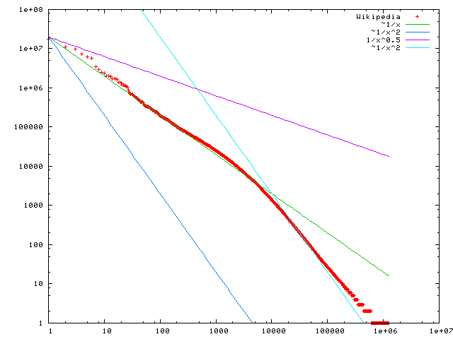
?figurename? 7.2: Word frequency (y-axis in log scale) v.s Word frequency ranking (x-axis in log scale) in Wikipedia (extracted from Wikipedia [3] under LGPL license)

Because the clustering effect in the PDP different from LDA, the number of unique words and rare words generated by PDP in each document is significantly higher than the results from LDA. In contrast LDA only generates i.i.d words from a multinomial distribution, hence is unable to capture the properties of a power-law [23].

Figure 7.3 shows the graphical model of PYTM. Figure 7.3 shows a more precise illustration that breaks down each PDP generation step. The generation process of PYTM is given as follows. In LDA we generate $z_{m,l}$ and $w_{m,l}$ according to $H(z,w|\vec{\theta}_{m},\Phi)$, which is a bivariate distribution equivalent to $z\sim\vec{\theta}_{m}$, $w\sim\vec{\phi}_{z}$, and $\Phi$ is the matrix representation of the collection of $\vec{\phi}_{k}$ for all $k=1...K$. In PYTM we modify the process and take a variant of $H(z,w|\vec{\theta}_{m},\Phi)$, then sample $z_{m,l}$ and $w_{m,l}$ from the variant.

$\displaystyle\vec{\phi}_{k}$ $\displaystyle\sim Dirichlet(\vec{\beta})$ $\displaystyle\forall k=1...K$ $\displaystyle\vec{\theta}_{m}$ $\displaystyle\sim Dirichlet(\vec{\alpha})$ $\displaystyle\forall m=1...M$ $\displaystyle G_{m}$ $\displaystyle\sim PDP(\gamma,d,H(\cdot,\cdot|\vec{\theta}_{m},\Phi))$ $\displaystyle\forall m=1...M$ $\displaystyle(z_{m,l},w_{m,l})$ $\displaystyle\sim G_{m}$ $\displaystyle\forall m=1...M,\,l=1...L_{m}$

Note that as $\gamma$ approaches infinity, $G_{m}$ approaches $H$, so the process collapsed into regular LDA.

Below is another way of representing this process, similar to what is introduced in [23]. It breaks down the sampling part to Chinese Restaurant Process. For each word $w_{m,l}$ with index $l$ in each document $m$:
$\displaystyle r_{m,l}$ $\displaystyle\sim Bernoulli(\frac{\gamma+dJ_{m}}{\gamma+l})$ $\displaystyle x_{m,l}$ $\displaystyle=\begin{cases}\mbox{$x_{m,s}$}\mbox{for some $1\leq s\leq l-1$, each with probability $\frac{n_{m,s}-\gamma}{d+l-1}$}&(r_{m,l}=0)\\ J_{m}+1&(r_{m,l}=1)\end{cases}$ $\displaystyle z_{m,l}$ $\displaystyle=\begin{cases}z_{m,s}&(r_{m,l}=0)\\ \mbox{Draw from }Multi(\vec{\theta}_{m})&(r_{m,l}=1)\end{cases}$ $\displaystyle v_{m,x_{m,l}}$ $\displaystyle=\begin{cases}\mbox{unchanged}&(r_{m,l}=0)\\ \mbox{Draw from }Discrete(\vec{\phi}_{z_{m,l}})&(r_{m,l}=1)\end{cases}$ $\displaystyle w_{m,l}$ $\displaystyle=v_{m,x_{m,l}}$ where: $\gamma$ is the concentration parameter of PDP, $d$ is the discount parameter of PDP. $K$ is total number of topics, $M$ is total number of documents. $J_{m}$ is number of distinct words so far in document $m$. Through out the process there are two types of generated words: either (1) when $r_{m,l}=0$, reuse a topic $k$ or word already generated from $\vec{\theta}_{m}$ or $\vec{\phi}_{k}$ before, or (2) when $r_{m,l}=1$, a new topic $z_{m,l}$ and a new word $w_{m,l}$ is generated from $\vec{\theta}_{m}$ and $\vec{\phi}_{k}$ directly (which can be same as a topic or word generated before, or completely new). $x_{m,l}$ and $v_{m,x_{m,l}}$ are defined as: If we put type (2) words into a sequence $\{v_{x_{m,l}}\}_{m}$ for each document $m$, and label them consecutively, $x_{m,l}$ is then the label for each word $w_{m,l}$. Since type (1) word only reuses word that already appeared before, they share the same label with same type (2) word. New topic $z_{m,l}$ is only generated for type (2) word.

?figurename? 7.3: PYTM graphical model

Figure 7.4: PYTM graphical model breakdown

The generation process of PYTM can also be described by a much simpler Chinese Restaurant Process (CRP) analogy of Poisson Dirichlet Process. We will give an overview of Poisson Dirichlet Process and the CRP analogy in the next section.

7.3 Hierarchical Pitman-Yor Topic Modelling (HPYTM)

The Hierarchical Pitman-Yor Topic Modelling (HPYTM) [23] made one extension to PYTM by assuming the power-law phenomenon not only exists in each document but also within each topic. PDP word generation is now document-topic specific instead of only document-specific as it is in PYTM. In this setup, new words (type (2) words) are no longer drawn from $Discrete(\vec{\phi}_{z_{m,l}})$, instead they are drawn from a distribution generated by PDP for a specific topic. The Hierarchical Bayesian Language Model [26] replaces some parts of PYTM still inheriting some features of LDA with a more complicated structure, as illustrated in Figure 7.3 and 7.6. Note $\vec{\beta}$ and $\vec{\phi}$ in PYTM have been replaced by a two-tier hierarchical model.

The break-down generation process is same as the generation process in PYTM, except for $v_{m,x_{m,l}}$:

$$v_{m,x_{m,l}}=\begin{cases}\mbox{unchanged}&(r_{m,l}=0)\\ \mbox{Draw from }Discrete(\vec{\phi}_{z_{m,l}})&(r_{m,l}=1)\end{cases}$$

And in addition:

$\displaystyle d_{k}$ $\displaystyle\sim Beta(a_{d},b_{d})$ $\displaystyle\forall k=1,...,K$ $\displaystyle\gamma_{k}$ $\displaystyle\sim Gamma(a_{\gamma},b_{\gamma})$ $\displaystyle\forall k=1,...,K$ $\displaystyle\vec{\phi}_{k}$ $\displaystyle\sim PDP(\gamma_{k},d_{k},\vec{\phi}_{0})$ $\displaystyle\forall k=1,...,K$ $\displaystyle\vec{\phi}_{0}$ $\displaystyle\sim PDP(\gamma_{0},d_{0},U)$

Where $a_{d},b_{d},a_{\gamma},b_{\gamma},\gamma_{0},d_{0}$ are all hyper-parameters, $U$ is a discrete uniform distribution ($\forall w:p(w)=1/V$).

?figurename? 7.5: HPYTM graphical model

Figure 7.6: HPYTM graphical model breakdown

7.4 Differential Topic Modelling Using Shadow Poisson Dirichlet Process

This differential model [2] addresses the problem of comparing multiple groups of documents. Differential topic models extend standard topic models by giving the model the ability to find similarities and differences in topics among multiple groups of documents. In this setup, the input documents are organized into multiple groups sharing the same vocabulary. Topics are shared across all groups but each group has their own representation of each topic. In addition, each group is allowed to have their unique topics.

In standard topic modelling, the sources of documents are not differentiated. In other words, all documents are assumed to be in the same group. This assumption simplifies the mathematical formulation of the topic model and the predictive probabilities, but with such assumption in place, topic models are unable to extract information on the variation in popularity of topics and words among multiple sources of documents. The differential information is important because it allows us to analyze subtle differences in opinions and perspectives across multiple collection of documents.

Here is an example to illustrate the power of differential topic models: consider a situation where we need to analyze articles gathered from two media outlets, one from Israel and one from Palestine. Apparently, Israeli editors are more likely to use the word “terrorism” to describe the Israeli-Palestinian conflict, because of some extreme measures used by some Palestine. In contrast, Palestinians editors are likely to use “aggression” to describe this topic, because they see Israeli as invaders to their homeland. When standard topic models are applied to both groups of documents individually, there is no guarantee that the same topic can be extracted from both groups. When standard topic models are applied to the whole collection of two groups of documents, they are more likely to mix Israeli-Palestinian issues into one topic, hence unable to provide differential analysis. Differential topic models are able to find both the shared topics among both groups, and different descriptions to such topics should they exist.

Combining the essence of all models introduced above and results from other mathematics research and topic modelling research, especially the theoretical results in [24], the improved PDP table-configuration sampler in [27], and the Hierarchical Dirichlet Process model [28], the Differential Topic Model with Shadow Poisson Dirichlet Process (SPDP) is born. This model outperforms many existing models in differential topic modelling context when the performance is measured in perplexity.

Although the superiority of this model has already been demonstrated in experiments, [2] does not provide an in depth explanation of the intuition of the model and derivation of the model. Since the rest of the thesis is entirely based on this model, in the following discussions I give an step-by-step explanation of this model.

Similar to the structure in HPYTM, each word-topic distribution is assumed to be generated from a base distribution $\vec{\phi}_{k}^{0}$. Assume the total vocabulary size is $V$. Each group is attached with a $V\times V$ transformation matrix $P^{i}$ that transforms the shared base distribution $\vec{\phi}_{k}^{0}$, represents the similarity between each pair of words, such that the sum of each row or column in $P^{i}$ is $1$. As a consequence, different transformation matrices introduce different word correlations for each group, so when words are generated, each group produces slightly different words for a common topic. The graphical model is given in 7.7. The generation process is as follows. The technical details of this model are left to next section, Model Derivation and Gibbs Sampler.

$\displaystyle\vec{\phi}_{k}^{0}$ $\displaystyle\sim Dirichlet(\vec{\beta})$ $\displaystyle\forall k=1,...,K$ $\displaystyle\vec{\phi}_{k}^{i}$ $\displaystyle\sim PDP(\gamma_{k},d_{k},P^{i}\vec{\phi}_{k}^{0})$ $\displaystyle\forall k=1,...,K,\,\forall i=1,...,I$ $\displaystyle\vec{\theta}_{i}^{d}$ $\displaystyle\sim Dirichlet(\vec{\alpha}_{i})$ $\displaystyle\forall i=1,...,I,\,\forall d=1,...,D_{i}$ $\displaystyle z_{id}^{l}$ $\displaystyle\sim Discrete(\vec{\theta}_{i}^{d})$ $\displaystyle\forall i=1,...,I,\,\forall d=1,...,D_{i},\,\forall l=1,...,L_{i,d}$ $\displaystyle w_{id}^{l}$ $\displaystyle\sim Discrete(\vec{\phi}_{z_{id}^{l}}^{i})$ $\displaystyle\forall i=1,...,I,\,\forall d=1,...,D_{i},\,\forall l=1,...,L_{i,d}$

Where $I$ is number of groups, $P^{i}$ is the transformation matrix for group $i$. $D_{i}$ is number of documents in group $i$. $L_{i,d}$ is document length of document $d$ in group $i$.

Figure 7.7: SPDP graphical model

The differential topic model SPDP is one particular representative of perhaps another hundred extensions of LDA. When combined with other algorithms and models, it has even more potential applications in practice, For instance, in many real world situations, group labels on collections of document are not accurately given. Many blogs and articles are shared around many websites on the Internet, without providing any reliable label of originality, category, or perspective. The majority of documents on the Internet (including social network messages such as tweets) are not tagged. Furthermore, tags do not always provide accurate information. Multiple documents sharing the same tag may belong to different categories or be written in different perspectives, hence do not necessarily belong to the same group. For example, a document tagged with “machine learning” could be in “reinforcement learning”, “topic modelling”, or other categories; a document tagged with “politics” could be either “left” or “right” depending on its perspective. It is desirable to have an algorithm that automatically classifies documents into different categories and perspectives, free from human influence and judgements. Because the differential topic model SPDP provide a fundamental framework based on groups, it is a very suitable candidate for this task. For example, a simple and naive solution is to iteratively use the topic probabilities and word probabilities across multiple groups generated by SPDP as features for machine learning algorithms such as Expectation Maximization (EM) to classify documents belonging to multiple unknown groups.

8 Model Derivation and Gibbs Sampler

All topic models mentioned in last section share some similarities in their derivations and inference processes, because fundamentally all of them are extensions of LDA. The collapsed Gibbs sampler is most frequently chosen by authors of above models to make inference on the multivariate latent variables. Although different models have different latent variables, for simplicity, we denote all of them by one latent parameter $\vec{\theta}\in\Theta_{latent}$. The goal is to make inference on the latent parameter (which include topic information) by estimating the Bayesian posterior of latent parameters (for example in LDA, word distributions $\phi_{k}$, and topic distributions $\theta_{m}$) given some data, according to Bayes’ rule:

$$p(\vec{\theta}|data)=\frac{p(\vec{\theta},data)}{p(data)}$$

Simply applying this formula often gives an intractable probability distribution for $p(\vec{\theta}|data)$. To see this, consider the simplest LDA model. To infer the latent topic assignment variable $\vec{z}$:

$$p(\vec{z}|\vec{w})=\frac{p(\vec{z},\vec{w})}{p(\vec{w})}=\frac{\prod_{l=1}^{L}p(z_{l},w_{l})}{\prod_{l=1}^{L}\sum_{k=1}^{K}p(z_{l}=k,w_{l})}$$

There are $K^{L}$ terms in the denominator, making the probability mathematically intractable.

However, if we are given a large number of samples from this probability distribution, we may find a number of ways to estimate the latent variables $\vec{\theta}$. Suppose we have samples $\vec{x}_{1},..\vec{x}_{n}$ from $p(\vec{\theta}|data)$. The easiest way to estimate it is to simply calculate the average occurrence of each possible outcome:

$$\hat{p}(\vec{\theta}|data)=\frac{1}{n}\sum_{i=1}^{n}\delta_{\vec{\theta}}(\vec{x}_{i})$$

Where $\vec{x}_{i}$ are the observed samples. The collapsed Gibbs sampler is used for this computation. The collapsed Gibbs sampler is an iterative sampler that generate random samples of a joint multivariate probability distribution $p(\vec{x})$ given $p(x_{i}|\vec{x}_{-i})$ is known. Here $\vec{x}_{-i}$ denotes $\vec{x}$ with element $x_{i}$ deleted. The collapsed Gibbs sampler requires a large number iterations for convergence. It starts with an arbitrary initial value for each $x_{i}$, sample each element $x_{i}$ from $p(x_{i}|\vec{x}_{-i})$ in each iteration, and update the value of $x_{i}$ as soon as it is sampled. The probability of samples $\vec{x}$ drawn in each iteration will almost surely converge to $p(\vec{\theta}|data)$. The proof can be found in most advanced statistics textbooks, such as [29].

In our settings, usually the quantity $p(\theta_{i}|\theta_{-i},data)$ can be easily deduced by computing:

$$p(\theta_{i}|\theta_{-i},data)=\frac{p(\vec{\theta},data)}{p(\theta_{-i},data)}$$ (8.1)

In topic modelling this is often referred as the predictive probability. To make our method work, we need a neat way to compute the predictive probability which is derived from the the joint distribution of the latent parameter and the data. In the rest of this section, we will show the derivation process of joint distribution and predictive probability for most models we described in last section.

For most of these models, we have written a step by step derivation. For the basic LDA model, we only explain the important steps and provided references to existing publications, to help readers find more detailed explanation.

8.1 Notation

Across this section, we use $V$ to denote the size of the vocabulary, $K$ to denote the total number of topics, $M$ to denote total number of documents, $n_{mk:m,k}$ to denote number of times topic $k$ observed in document $m$, where the first part of subscript is a label to distinguish it from other counting variables that may also be named with $n$, and $n_{kw:k,w}$ to denote number of times word $w$ associated with topic $k$. We use $n_{kw:k,.}$ to denote the sum over dotted variables in the subscript, for example, $n_{kw:k,.}=\sum_{w=1}^{V}n_{kw:k,w}$, and similarly $n_{mk:m,.}=\sum_{k=1}^{K}n_{mk:m,k}$.

8.2 Latent Dirichlet Allocation (LDA)

The joint distribution $p(\vec{\theta},data)$ of LDA can be represented as

$$p(\vec{w},\vec{z}|\vec{\alpha},\vec{\beta})=p(\vec{w}|\vec{z},\vec{\beta})p(\vec{z}|\vec{\alpha})$$ (8.2)

Since $\vec{z}$ is not dependent on $\vec{\beta}$. The first term $p(\vec{w}|\vec{z},\vec{\beta})$ in 8.2 can be derived as:

$\displaystyle p(\vec{w}|\vec{z},\vec{\beta})$ $\displaystyle=$ $\displaystyle\int_{\vec{\phi}}p(\vec{w}|\vec{z},\vec{\phi})p(\vec{\phi}|\vec{\beta})d\vec{\phi}$ (8.3) $\displaystyle=$ $\displaystyle\int_{\vec{\phi}}\prod_{k=1}^{K}\frac{1}{\Delta(\vec{\beta})}\prod_{w=1}^{V}\phi_{k,w}^{n_{k,w}+\beta_{w}-1}d\vec{\phi}$ $\displaystyle=$ $\displaystyle\prod_{k=1}^{K}\frac{\Delta(\vec{\beta}+\vec{n}_{k})}{\Delta(\vec{\beta})}$

Where $n_{k,w}$ is a counting variable representing number of terms in all documents that have been assigned to topic $k$ and word $w$. $\Delta(\vec{x})$ is the Dirichlet delta function, the normalizing constant, as defined in [21]:

$$\Delta(\vec{x})=\frac{\prod_{k=1}^{\dim\vec{x}}\Gamma(x_{k})}{\Gamma(\prod_{k=1}^{\dim\vec{x}}(x_{k}))}$$

Similarly, the second term $p(\vec{z}|\vec{\alpha})$ in 8.2 can be derived as:

$\displaystyle p(\vec{z}|\vec{\alpha})$ $\displaystyle=$ $\displaystyle\int_{\vec{\theta}}p(\vec{z}|,\vec{\theta})p(\vec{\theta}|\vec{\alpha})d\vec{\theta}$ (8.4) $\displaystyle=$ $\displaystyle\int_{\vec{\theta}}\prod_{d=1}^{M}\frac{1}{\Delta(\vec{\alpha})}\prod_{k=1}^{K}\theta_{m,k}^{n_{m,k}+\alpha_{k}-1}d\vec{\theta}$ $\displaystyle=$ $\displaystyle\prod_{k=1}^{M}\frac{\Delta(\vec{\alpha}+\vec{n}_{m})}{\Delta(\vec{\beta})}$

Where $n_{m,k}$ is a counting variable representing number of terms in document $m$ that have been assigned with topic $k$. Putting equations 8.28.38.4 together:

$\displaystyle p(\vec{w},\vec{z}|\vec{\alpha},\vec{\beta})$ $\displaystyle=$ $\displaystyle p(\vec{w}|\vec{z},\vec{\beta})p(\vec{z}|\vec{\alpha})$ (8.5) $\displaystyle=$ $\displaystyle\prod_{k=1}^{K}\frac{\Delta(\vec{\beta}+\vec{n}_{k})}{\Delta(\vec{\beta})}\prod_{k=1}^{M}\frac{\Delta(\vec{\alpha}+\vec{n}_{m})}{\Delta(\vec{\beta})}$

Substitutes 8.5 into 8.1 :

$\displaystyle p(z_{i}=k|\vec{w},\vec{z}_{-i},\vec{\alpha},\vec{\beta})$ $\displaystyle=$ $\displaystyle\frac{p(\vec{w},\vec{z})}{p(\vec{w},\vec{z}_{-i})}$ $\displaystyle=$ $\displaystyle\frac{p(\vec{w}|\vec{z})}{p(\vec{w}_{-i},\vec{z}_{-i})}\frac{p(\vec{z})}{p(w_{i})}$ $\displaystyle\propto$ $\displaystyle\frac{\Delta(\vec{\beta}+\vec{n}_{k})}{\Delta(\vec{\beta}+\vec{n}_{k,-i})}\frac{\Delta(\vec{\alpha}+\vec{n}_{m})}{\Delta(\vec{\alpha}+\vec{n}_{m,-i})}$ $\displaystyle\propto$ $\displaystyle\frac{\Gamma(n_{k,w}+\beta_{w})\Gamma(\sum_{w=1}^{V}(n_{k,w,-i}+\beta_{w}))}{\Gamma(n_{k,w,-i}+\beta_{w})\Gamma(\sum_{w=1}^{V}(n_{k,w}+\beta_{w}))}\frac{\Gamma(n_{m,k}+\alpha_{k})\Gamma(\sum_{k=1}^{K}(n_{m,k,-i}+\alpha_{k}))}{\Gamma(n_{m,k,-i}+\alpha_{k})\Gamma(\sum_{k=1}^{K}(n_{m,k}+\alpha_{k}))}$ $\displaystyle\propto$ $\displaystyle\frac{n_{k,w,-i}+\beta_{w}}{\sum_{w=1}^{V}(n_{k,w,-i}+\beta_{w})}\frac{n_{m,k,-i}+\alpha_{k}}{\sum_{k=1}^{K}(n_{m,k,-i}+\alpha_{k})-1}$

Where a variable with subscript $-i$ denotes the value of such variable with element $i$ (word $i$) is removed. Above formula gives the proportional predictive probability for the collapsed Gibbs sampling. For more detailed explanation on LDA, readers should refer to [1].

8.3 Pitman-Yor Topic Modelling (PYTM)

8.3.1 Poisson Dirichlet Process

We first give an overview of the Poisson Dirichlet Process (PDP) as it is the foundation of PYTM. As mentioned in the last section, PDP generates a probability distribution from a base distribution $H(.)$, concentration parameter $\gamma$, and discount parameter $d$. The process is denoted by $PDP(\gamma,d,H(.))$. The Chinese Restaurant analogy is as follows: In a strange Chinese restaurant which has infinite number of tables, each table serves only one dish, and only when at least one customer is sitting on that table. Waiters will arrange each incoming customer to either sit in a table served with dish $j$, share it among other people who are already sitting there, or lead the customer to an empty table and immediately serve a dish. Waiters keep a record of the number of distinct dishes $1,...,J$ served to customers, the number of customers served with dish $j$, denoted by $n_{j}$, and the total number of customers, denoted by $N$. They use the following procedure to make seating arrangements for each incoming customer:

• Take the customer to an empty table with probability $\frac{\gamma+dJ}{\gamma+N}$, and serve some dish $j$ drawn from $H(.)$

• Otherwise, take the customer to some table already serving dish $j$, with probability $\frac{n_{j}-d}{\gamma+N}$ in total for all these tables

Samples drawn from the distribution generated by the PDP can be understood as the dishes served to each customer. In the PYTM model (Figure 7.3 ), a restaurant is created for each document. Each word in the document is a customer coming to the restaurant. Each different word in the vocabulary is an unique type of dish. $x_{m,l}$ records which table the customer sat in. $v_{m,s}$ records the dish being served at table $s$ in restaurant $m$. $z_{m,s}$ records the topic associated with table $s$ in restaurant $m$. The observed words $w_{m,l}=v_{m,x_{m,l}}$ are the samples drawn from the distribution generated from PDP.

The formal definition of the Poisson Dirichlet Process is a sequence of draws from the base distribution $H(.)$ coupled with probability weighting vector $\vec{p}$ drawn from Poisson Dirichlet Distribution as stated in [30]. A detailed Bayesian analysis of Poisson Dirichlet Process is given in [24] by Buntine and Hutter. Because their works are highly technical, far above the level of this thesis, and they are not directly related to topic modelling, we only use only some of their results and only show the derivation when necessary.

Following the analogy we can immediately get the predictive probability of which dish would be served to an incoming customer:

$$p(x_{i}=j|x_{1},x_{2},...,x_{i-1},\gamma,d,H(.))=\frac{n_{j}-d}{\gamma+N}+\frac{\gamma+dJ}{\gamma+N}H(j)$$

8.3.2 Predictive Probability and Inference

Predictive probability can be derived by removing a word, similar to LDA. Here we need both topic predictive probability and word predictive probability to proceed with inference, because when we remove a word, we add it back later, and we need to reconsider the sitting arrangement when add it back. Luckily the word predictive probability is directly given by CRP analogy because in above definition each word drawn is dependent on all previous words drawn : $$p(w_{m,l}=j|\boldsymbol{W},\boldsymbol{Z},\boldsymbol{X})=\frac{n_{mw:m,j}-d}{\gamma+n_{mw:m.}}+\frac{\gamma+dJ_{m}}{\gamma+n_{mw:m.}}\sum_{k=1}^{K}\frac{n_{m,k}+\alpha_{m}}{n_{m}+\alpha_{m:.}}\frac{n_{kw:k,j}+\beta_{k}}{n_{kw:k,.}+\beta_{k:.}}$$ (8.6)

Where $n_{mj:m,j}$ is number of times word $w$ appeared in document $m$ (not including $w_{m,l}$), $n_{mw:m.}$is number of words observed so far in document $m$ without $w_{m,l}$, $\boldsymbol{W},\boldsymbol{Z},\boldsymbol{X}$ are words, topics, sitting arrangements not including $w_{m,l}$ or anything associated with $w_{m,l}$. $H(.)$ is replaced by the summation term, which is borrowed from LDA word predictive probability as for this part they share the same word generation procedure (see figure 7.4 and the breakdown generation illustration.)

Similarly, the topic predictive probability is given by

$$p(z_{m,l}=k|\boldsymbol{W},\boldsymbol{Z},\boldsymbol{X},w_{m,l}=j,x_{m,l}=s)=\frac{n_{mk:m,k}+\alpha_{m}}{n_{mk:m,.}+\alpha_{m:.}}\frac{n_{kw:k,j}+\beta_{k}}{n_{kw:k,.}+\beta_{k:.}}$$

as derived in LDA.

8.4 Hierarchical Pitman-Yor Topic Modelling (HPYTM)

The derivation process is almost same as described in PYTM, except probabilities are computed recursively. We will skip this section as the detail is not particularly related to SPDP. Readers should refer to [23] if they are interested in the details.

8.5 Shared Topic Modelling Using Shadow Poisson Dirichlet Process

As mentioned in the last section the Shadow Poisson Dirichlet Process (SPDP) is in fact a Poisson Dirichlet Process coupled with linearly transformed base measure. One important property we used to derive the predictive probability in LDA is Dirichlet distribution is conjugate to Discrete (categorical, or multinomial) distribution. The same property is used in PYTM and its extension HPYTM as they use LDA as a foundation. In this model the same method does not apply because the transformed base measure is no longer conjugate to a Discrete (categorical, or multinomial) distribution.

To overcome this, first we introduce auxiliary variable $t_{i,k,w}$, which we refer as multiplicity, represents number of tables served with dish $w$ in restaurant $i,k$ (group $i$, topic $k$). It is shown by Corollary 17 in [24] that in one “restaurant”:

$$p(\vec{w},\vec{t}|\gamma,d,H(.))=\frac{(\gamma|d)_{t_{.}}}{(d)_{n_{.}}}\prod_{j=1}^{J}(H(w_{j}^{\star})^{t_{j}}S_{t_{j},\gamma}^{n_{j}})$$

Where $J$ is the number distinct dishes, $\vec{w}$ is dish served to each customer and $\vec{t}$ is the multiplicity of each dish. $(w_{1}^{\star},...,w_{j}^{\star})$ is the sequence of distinct dishes. $t_{.}$ is the sum of multiplicities, equivalent to total number of non-empty tables. $n_{j}$ is number of customers having dish $j$, and $n_{.}$ is equivalent to total number of customers. $(x|y)_{N}$ and $(x)_{N}$ are Pochhammer symbol, where $(x|y)_{N}=\prod_{n=0}^{N-1}(x+ny)$, and $(x)_{N}=(x|1)_{N}$. $S_{M,a}^{N}$ is a generalized Sterling number, given by linear recursion $S_{M,a}^{N+1}=S_{M-1,a}^{N}+(N-Ma)S_{M,a}^{N}$ and $S_{M,a}^{N}=0$ for $M>N$, $S_{0,a}^{N}=\delta_{N,0}$. Both generalized Sterling numbers and Pochhammer symbols can be computed and cached efficiently before the Gibbs sampling process starts.

In our settings $H(w_{j}^{\star})$ is replaced by the probability $\phi_{v}^{0}$. After transformation the base distribution becomes $P^{i}\vec{\phi}^{0}$, and $\phi_{w}^{0}=\sum_{v}p_{w,v}\phi_{v}^{0}$ where $p_{w,v}$ denotes element of the matrix. Therefore:

$$p(\vec{w},\vec{t}|\gamma,d,\vec{\phi}^{0})=\frac{(\gamma|d)_{t_{.}}}{(d)_{n_{.}}}\prod_{j=1}^{J}S_{t_{j},\gamma}^{n_{j}}(\sum_{v}p_{w,v}\phi_{v}^{0})^{t_{j}}$$ (8.7)

It is clear the summation term inside the product has to be simplified. Chen et al. introduced two solutions for this problem: blocked Gibbs sampling, and hybrid Gibbs sampling with variational method.

The hybrid Gibbs with variational method approximates the above equation by deriving an inequality for above equation with $\vec{\phi}$ integrated out, then introduces another variable $q_{w,v}=\frac{p_{w,v}\phi_{v}^{0}}{\sum_{v^{\prime}}p_{w,v^{\prime}}\phi_{v^{\prime}}^{0}}$ that can be substituted to the lower bound. By using Jensen’s inequality and a Lagrange multiplier, it can be shown that $q_{w,v}$ maximize previously derived inequality after substitution. As the summation term is simplified, one then derive the sampling predictive probabilities as usual with equation 8.1. The latent variables such as word probability $\phi_{k,v}^{0}$ , can be computed by

$$\phi_{k,v}^{0}=e^{\psi(\gamma_{v}+\sum_{i}\sum_{w}q_{k,w,v}^{i}t_{i,k,w})}/\sum_{v}e^{\psi(\gamma_{v}+\sum_{i}\sum_{w}q_{k,w,v}^{i}t_{i,k,w})}$$ (8.8)

where $\psi$ is the digamma function. However, experiements have shown this approximation is not very accurate, as error accumulates the performance of the algorithm degrades significantly. Therefore in the rest of this section we will be concentrating on the first method: blocked Gibbs sampling.

In equation 8.7 suppose for each word $w$ we have another auxilliary variable $\vec{v}$ which has dimension $t_{w}$, the multiplicity of the word in one PDP process. We need $\vec{v}$ to separate the power term $(\sum_{v}p_{w,v}\phi_{v}^{0})^{t_{j}}$ into this form $(\sum_{v_{1}}p_{w,v_{1}}\phi_{v}^{0})(\sum_{v_{2}}p_{w,v_{2}}\phi_{v_{2}}^{0})...(\sum_{v_{t_{w}}}p_{w,v_{t_{w}}}\phi_{v_{t_{w}}}^{0})$, such that the terms inside each bracket is dependent on $v_{i}$ and its effect is marginalized out in 8.7. If we compute the joint probability as in equation 8.7 with some $\vec{v}$ we will get:

$$p(\vec{w},\vec{t},\vec{v}|\gamma,d,\vec{\phi}^{0})=\frac{(\gamma|d)_{t_{.}}}{(d)_{n_{.}}}\prod_{j=1}^{J}S_{t_{j},\gamma}^{n_{j}}\prod_{s=1}^{t_{w}}p_{w,v_{s}}\phi_{v_{s}}^{0}$$ (8.9)

Which is much simpler than 8.7, simple enough to be efficiently computed in logarithm space.

Because of the dimensionality difference between $\vec{w}$ and $\vec{v}$, to make use of the auxilliary variable $\vec{v}$ we need another auxilliary variable $\vec{r}$ called table indicator that has same dimension as $\vec{w}$ , constructed as follows: for each word (customer) $w_{i,d,l}$ we set $r_{i,d,l}=1$ if the word has created a new table (the customer is arranged to an empty table and served a new dish), otherwise we set $r_{i,d,l}=0$. For every word $w_{i,d,l}$ such that $r_{i,d,l}=1$ we associate the word with $v_{i,k,w,t}$ where $t$ is the table index of the word. $\vec{r}$ coupled with $\vec{t}$ provides more information than $\vec{t}$ alone because $\vec{r}$ in a specific seating configuration to each word in the document and $\vec{t}$ disregards the information of which word is creator of the table. For each table configuration specified by $\vec{t}$, there are $\prod_{v=1}^{V}\begin{pmatrix}n_{v}\\ t_{v}\end{pmatrix}$ different configurations of $\vec{r}$, thus

$$p(\vec{w},\vec{t}|\gamma,d,\vec{\phi}^{0})=\prod_{v=1}^{V}\begin{pmatrix}n_{v}\\ t_{v}\end{pmatrix}p(\vec{r},\vec{t}|\gamma,d,\vec{\phi}^{0})$$ (8.10)

Now we are ready to deduce a joint likelihood of these variables, which afterwards can be easily transformed into a predictive probability using 8.1 : $\displaystyle p(\mathbf{W},\mathbf{Z},\mathbf{V},\mathbf{R}|\vec{\gamma},\vec{d},\vec{\alpha_{1:I}},\vec{\beta},\mathbf{P})$ $\displaystyle=$ $\displaystyle\int_{\Phi}p(\mathbf{W},\mathbf{Z},\mathbf{V},\mathbf{R}|\vec{\phi}_{1:K}^{0},\vec{\gamma},\vec{d},\vec{\alpha}_{1:I},\mathbf{P})p(\vec{\phi}_{1:K}^{0}|\vec{\beta})d\Phi$ $\displaystyle=$ $\displaystyle p(\mathbf{Z}|\vec{\alpha}_{1:I})\int_{\Phi}p(\mathbf{W},\mathbf{V},\mathbf{R}|\mathbf{Z},\vec{\phi}_{1:K}^{0},\vec{\gamma},\vec{d},\mathbf{P})p(\vec{\phi}_{1:K}^{0}|\vec{\beta})d\Phi$

Where $\Phi$ is the collection of $\vec{\phi}_{1:K}^{0}$. Let $\Theta$ be the collection of $\vec{\theta}_{1:I,1:D}$, then

$\displaystyle p(\mathbf{Z}|\vec{\alpha}_{1:I})$ $\displaystyle=$ $\displaystyle\int_{\Theta}p(\mathbf{Z}|\Theta)p(\Theta|\vec{\alpha}_{1:I})d\Theta$ $\displaystyle=$ $\displaystyle\int_{\Theta}\prod_{i=1}^{I}\prod_{d=1}^{D}\frac{1}{Beta_{K}(\vec{\alpha}_{i})}\prod_{k=1}^{K}\theta_{i,d,k}^{n_{idk:i,d,k}}\theta_{i,d,k}^{\alpha_{i,k}-1}d\Theta$ $\displaystyle=$ $\displaystyle\prod_{i=1}^{I}\prod_{d=1}^{D}\frac{Beta_{K}(\vec{\alpha}_{i}+\vec{n}_{idk:i,d})}{Beta_{K}(\vec{\alpha}_{i})}$

Where $\vec{n}_{idk:i,d}=(n_{idk:i,d,1},n_{idk:i,d,2},...,n_{idk:i,d,K})$. Substitute equation 8.9 and 8.10 into the terms inside the integral in LABEL:eq:SPDP-Blocked-Gibbs-Joint-Prob:

$\displaystyle p(\mathbf{W},\mathbf{V},\mathbf{R}|\mathbf{Z},\vec{\phi}_{1:K}^{0},\vec{\gamma},\vec{d},\mathbf{P})$ $\displaystyle=$ $\displaystyle\prod_{i=1}^{I}\prod_{k=1}^{K}\frac{(\gamma|d)_{t_{ikw:i,k,.}}}{(d)_{n_{ikw:i,k,.}}}$ $\displaystyle\bigg{(}\prod_{w=1}^{V}\begin{pmatrix}n_{w}\\ t_{w}\end{pmatrix}^{-1}S_{t_{ikw:i,k,j},\gamma_{k}}^{n_{ikj:i,k,j}}\prod_{s=1}^{t_{ikw:i,k,w}}p_{i,w,v_{s}}\phi_{k,v_{s}}^{0}\bigg{)}$ $\displaystyle p(\vec{\phi}_{1:K}^{0}|\vec{\beta})$ $\displaystyle=$ $\displaystyle\prod_{k=1}^{K}\frac{1}{Beta(\vec{\beta})}\prod_{w=1}^{V}(\phi_{k,w}^{0})^{\beta_{v}-1}$ (8.12)

With respect to $\Phi$ the integral in LABEL:eq:SPDP-Blocked-Gibbs-Joint-Prob can be easily evaluated as a multinomial probability density function. To simplify the result more, we introduce an auxilliar statistic $q_{i,k,w,v}=\sum_{t=1}^{t_{ikw:i,k,w}}1_{v_{i,k,w,t=v}}$, the number of tables associated (as defined by $v_{ikwt}$) with one particular word $v$ in a PDP process. By doing so, $\prod_{s=1}^{t_{ikw:i,k,w}}p_{i,w,v_{s}}\phi_{k,v_{s}}^{0}$ can be neatly rewritten as $\prod_{v=1}^{V}(p_{w,v}\phi_{k,v}^{0})^{q_{i,k,w,v}}$, thus:

$\displaystyle\int_{\Phi}p(\mathbf{W},\mathbf{V},\mathbf{R}|\mathbf{Z},\vec{\phi}_{1:K}^{0},\vec{\gamma},\vec{d},\mathbf{P})p(\vec{\phi}_{1:K}^{0}|\vec{\beta})d\Phi$ $\displaystyle=$ $\displaystyle\int_{\Phi}(\prod_{i=1}^{I}\prod_{k=1}^{K}\frac{(\gamma|d)_{t_{ikw:i,k,.}}}{(d)_{n_{ikw:i,k,.}}}\prod_{w=1}^{V}\begin{pmatrix}n_{w}\\ t_{w}\end{pmatrix}^{-1}S_{t_{ikw:i,k,j},\gamma_{k}}^{n_{ikj:i,k,j}}\prod_{s=1}^{t_{ikw:i,k,w}}p_{i,w,v_{s}}\phi_{v_{s}}^{0})$ $\displaystyle\prod_{k=1}^{K}\frac{1}{Beta(\vec{\beta})}\prod_{w=1}^{V}(\phi_{k,w}^{0})^{\beta_{w}-1}d\Phi$ (8.13) $\displaystyle=$ $\displaystyle\int_{\Phi}\prod_{k=1}^{K}\frac{1}{Beta(\vec{\beta})}(\prod_{i=1}^{I}\frac{(\gamma|d)_{t_{ikw:i,k,.}}}{(d)_{n_{ikw:i,k,.}}}\prod_{w=1}^{V}\begin{pmatrix}n_{w}\\ t_{w}\end{pmatrix}^{-1}S_{t_{ikw:i,k,j},\gamma_{k}}^{n_{ikj:i,k,j}}$ $\displaystyle\prod_{v=1}^{V}(\phi_{k,v}^{0})^{q_{i,k,w,v}+\beta_{w}-1}(p_{w,v})^{q_{i,k,w,v}})d\Phi$ (8.14) $\displaystyle=$ $\displaystyle\prod_{k=1}^{K}\frac{1}{Beta(\vec{\beta})}\bigg{(}(\prod_{i=1}^{I}\frac{(\gamma|d)_{t_{ikw:i,k,.}}}{(d)_{n_{ikw:i,k,.}}}\prod_{w=1}^{V}\begin{pmatrix}n_{w}\\ t_{w}\end{pmatrix}^{-1}S_{t_{ikw:i,k,j},\gamma_{k}}^{n_{ikj:i,k,j}}\bigg{)}$ $\displaystyle\bigg{(}\int_{\Phi}\prod_{i=1}^{I}\prod_{w=1}^{V}\prod_{v=1}^{V}(\phi_{k,v}^{0})^{q_{i,k,w,v}+\beta_{w}-1}(p_{w,v})^{q_{i,k,w,v}})d\Phi)\bigg{)}$ (8.15)

Evaluate the integral, we get

$\displaystyle\prod_{k=1}^{K}\int_{\Phi}\prod_{i=1}^{I}\prod_{w=1}^{V}\prod_{v=1}^{V}(\phi_{k,v}^{0})^{q_{i,k,w,v}+\beta_{w}-1}(p_{w,v})^{q_{i,k,w,v}})d\Phi$ $\displaystyle=$ $\displaystyle(\prod_{i=1}^{I}\prod_{w=1}^{V}\prod_{v=1}^{V}(p_{w,v})^{\sum_{k=1}^{K}q_{i,k,w,v}})(\prod_{k=1}^{K}\frac{\prod_{i=1}^{I}Beta_{V}(\vec{\beta}+\sum_{i}\sum_{w}\vec{q}_{i,k,w})}{Beta_{V}(\vec{\beta})})$ (8.16)

Where in 8.13 we simply substituted values from equation 8.12. In 8.14 we re-wrote the terms in $q_{ikwv}$. In 8.15 we rearranged the equation. In 8.16 we took out $p_{w,v}$ and evaluated the integral as multinomial probability density function.

Finally, put all terms together:

$\displaystyle p(\mathbf{W},\mathbf{Z},\mathbf{V},\mathbf{R}|\vec{\gamma},\vec{d},\vec{\alpha_{1:I}},\vec{\beta},\mathbf{P})$ $\displaystyle=$ $\displaystyle\prod_{i=1}^{I}\prod_{d=1}^{D}\frac{Beta_{K}(\vec{\alpha}_{i}+\vec{n}_{idk:i,d})}{Beta_{K}(\vec{\alpha}_{i})}$ $\displaystyle\bigg{(}\prod_{k=1}^{K}(\prod_{i=1}^{I}\frac{(\gamma|d)_{t_{ikw:i,k,.}}}{(d)_{n_{ikw:i,k,.}}}\prod_{w=1}^{V}\begin{pmatrix}n_{w}\\ t_{w}\end{pmatrix}^{-1}S_{t_{ikw:i,k,j},\gamma_{k}}^{n_{ikj:i,k,j}})\bigg{)}$ $\displaystyle\bigg{(}\prod_{i=1}^{I}\prod_{w=1}^{V}\prod_{v=1}^{V}(p_{w,v})^{\sum_{k=1}^{K}q_{i,k,w,v}})(\prod_{k=1}^{K}\frac{\prod_{i=1}^{I}Beta_{V}(\vec{\beta}+\sum_{i}\sum_{w}\vec{q}_{i,k,w})}{Beta_{V}(\vec{\beta})}\bigg{)}$

And simplify a bit:

$\displaystyle p(\mathbf{W},\mathbf{Z},\mathbf{V},\mathbf{R}|\vec{\gamma},\vec{d},\vec{\alpha_{1:I}},\vec{\beta},\mathbf{P})$ $\displaystyle=$ $\displaystyle(\prod_{i=1}^{I}\prod_{w=1}^{V}\prod_{v=1}^{V}(p_{w,v})^{\sum_{k=1}^{K}q_{i,k,w,v}})(\prod_{i=1}^{I}\prod_{d=1}^{D}\frac{Beta_{K}(\vec{\alpha}_{i}+\vec{n}_{idk:i,d})}{Beta_{K}(\vec{\alpha}_{i})})$ $\displaystyle\bigg{(}\prod_{k=1}^{K}\big{(}\prod_{i=1}^{I}\frac{(\gamma|d)_{t_{ikw:i,k,.}}}{(d)_{n_{ikw:i,k,.}}}Beta_{V}(\vec{\beta}+\sum_{i}\sum_{w}\vec{q}_{i,k,w})\big{)}\bigg{)}$ $\displaystyle\bigg{(}\prod_{k=1}^{K}\frac{1}{Beta_{V}(\vec{\beta})}\prod_{i=1}^{I}\prod_{w=1}^{V}\begin{pmatrix}n_{w}\\ t_{w}\end{pmatrix}^{-1}S_{t_{ikw:i,k,j},\gamma_{k}}^{n_{ikj:i,k,j}})\bigg{)}$

Although the derivation of joint probability is a bit complicated and requires a significant amount of work, the inference steps are quite simple and efficient. In blocked Gibbs sampling, we sample multiple variables together in one step, one element each. In our settings the best choice is to sample one element each from $z,r,v$ together: for each word $w$, if $r=0$, we can simply ignore the value of $v$ and compute the probability of $(z=k,r=0)$, otherwise we compute the probability of $(z=k,r=1,v_{w}=v)$. Use the joint probability computed above and the formula 8.1:

$\displaystyle p(w_{i,d,l}=w,z_{i,d,l}=k,r_{i,d,l}=0|\mbox{ the rest with word $w$ removed$)$}$ $\displaystyle\propto$ $\displaystyle\frac{\alpha_{i,k}+n_{idk:i,d,k}}{b_{k}+m_{ikw:i,k\cdot}}\frac{m_{ikw:i,k,w}-t_{ikw:i,k,w}+1}{m_{ikw:i,k,w}+1}\frac{S_{t_{ikw:i,k,w},a_{k}}^{m_{ikw:i,k,w}+1}}{S_{t_{ikw:i,k,w},a_{k}}^{m_{ikw:i,k,w}}}$ (8.17)

$\displaystyle p(w_{i,d,l}=w,z_{i,d,l}=k,r_{i,d,l}=1,v_{i,k,w,t}=v|\mbox{ the rest with word $w$ removed$)$}$ $\displaystyle\propto$ $\displaystyle p_{i,w,v}(\alpha_{i,k}+n_{idk:i,d,k})\frac{b_{k}+a_{k}t_{ikw:i,k,\cdot}}{b_{k}+m_{ikw:i,k\cdot}}\frac{t_{ikw:i,k,w}+1}{m_{ikw:i,k,w}+1}\frac{\gamma_{v}+\sum_{i}\sum_{w}q_{i,k,w,v}}{\sum_{v^{\prime}}\gamma_{v^{\prime}}+\sum_{i}\sum_{w}t_{ikw:i,k,w}}\frac{S_{t_{ikw:i,k,w}+1,a_{k}}^{m_{ikw:i,k,w}+1}}{S_{t_{ikw:i,k,w},a_{k}}^{m_{ikw:i,k,w}}}$ (8.18)

The algorithm is illustrated in Algorithm 1.

1:for all $w_{i,d,l}$ in all documents in all groups do

2:     $k=z_{i,d,l}$, $w=w_{i,d,l}$

3:     Sample $r_{i,d,l}\sim Bernoulli(\frac{t_{ikw:i,k,w}}{m_{ikw:i,k,w}})$

4:     Decrement $n_{idk:i,d,k}$, $m_{ikw:i,k,w}$

5:     if $r_{i,d,l}\equiv 1$ then

6:         Decrement $t_{i,k,w}$

7:         Sample $t\sim Uniform(1,...,t_{ikw:i,k,w}+1)$

8:         Remove t-th element from linked list $\vec{v}_{ikw:i,k,w}$

9:         Decrement $q_{i,k,w,v}$

10:     end if

11:     for each topic k in 1…K do

12:         Compute following proportionalities for each v in 1…V:

13:         $z_{i,d,l}=k$, $r_{i,d,l}=0$:

14:         $\frac{\alpha_{i,k}+n_{idk:i,d,k}}{b_{k}+m_{ikw:i,k\cdot}}\frac{m_{ikw:i,k,w}-t_{ikw:i,k,w}+1}{m_{ikw:i,k,w}+1}\frac{S^{m_{ikw:i,k,w}+1}_{t_{ikw:i,k,w},a_{k}}}{S^{m_{ikw:i,k,w}}_{t_{ikw:i,k,w},a_{k}}}$

15:         $z_{i,d,l}=k$, $r_{i,d,l}=1$, $v_{i,k,w,t}=v$:

16:         $p_{i,w,v}(\alpha_{i,k}+n_{idk:i,d,k})\frac{b_{k}+a_{k}t_{ikw:i,k,\cdot}}{b_{k}+m_{ikw:i,k\cdot}}\frac{t_{ikw:i,k,w}+1}{m_{ikw:i,k,w}+1}\frac{\gamma_{v}+\sum_{i}{\sum_{w}{q_{i,k,w,v}}}}{\sum_{v^{\prime}}{\gamma_{v^{\prime}}}+\sum_{i}{\sum_{w}{t_{ikw:i,k,w}}}}\frac{S^{m_{ikw:i,k,w}+1}_{t_{ikw:i,k,w}+1,a_{k}}}{S^{m_{ikw:i,k,w}}_{t_{ikw:i,k,w},a_{k}}}$

17:     end for

18:     Jointly sample $z_{i,d,l}$, $r_{i,d,l}$, and $v_{i,k,w,t}$ according to proportionalities above.

19:     Increment $n_{idk:i,d,k}$, $m_{ikw:i,k,w}$

20:     if $r_{i,d,l}\equiv 1$ then

21:         Increment $t_{i,k,w}$ and $q_{i,k,w,v}$

22:         Add $v$ to linked list $\vec{v}_{ikw:i,k,w}$

23:     end if

24:end for

Algorithm 1 SPDP Full Gibbs Sampling

After convergence, the probability of a topic in a document can be estimated in the same way as in LDA, by taking expectation of the Dirichlet distribution:

$$\tilde{\theta}_{i,d,k}=\frac{n_{idk:i,d,k}+\alpha_{k}}{\sum_{k=1}^{K}(n_{idk:i,d,k}+\alpha_{k})}$$ (8.19)

And the probability of a topic can be estimated by taking the weighted sum of $\theta_{i,d,k}$ with document length as weight. The probability of a word in a topic can be esitmated by using the approximation of 8.8 with $q_{ikwv:i,k,w,v}t_{ikw:i,k,w}$ replaced by the exact count $q_{ikwv:i,k,w,v}$, and the posterier of PDP:

$\displaystyle\tilde{\phi}_{k,v}^{0}$ $\displaystyle=$ $\displaystyle\frac{\gamma_{v}+\sum_{i}\sum_{w}q_{ikwv:i,k,w,v}}{\sum_{v}\gamma_{v}+\sum_{v}\sum_{i}\sum_{w}q_{ikwv:i,k,w,v}}$ (8.20) $\displaystyle\tilde{\phi}_{k,w}^{i}$ $\displaystyle=$ $\displaystyle\frac{m_{ikw:i,k,w}-a_{k}t_{ikw:i,k,w}}{b_{k}+m_{ikw:i,k,\cdot}}+\frac{a_{k}t_{ikw:i,k,\cdot}}{b_{k}+m_{ikw:i,k,\cdot}}(\sum_{v}p_{w,v}^{i}\tilde{\phi}_{k,v}^{0})$ (8.21)

?chaptername? 3 Problems and Solutions

9 SPDP Computational Time Analysis

9.1 Theoretical Running Time Analysis

Assume there are $N$ words in total across all documents in all groups. Let $K$ represents the total number of topics to be extracted, and $V$ represents total number of words in the vocabulary. Furthermore, assume Gibbs sampler only converges after $T$ iterations. Algorithm 1 shows for each word, all topics and all possible word-associations must be sampled. Although Stirling numbers in the algorithm need to be computed recursively, it is possible to cache almost all of them before the algorithm begins, allowing constant-time retrieval complexity. To summarize, the theoretical worst case complexity of algorithm 1 is $\Theta(TNKV)$. As the transofrmation matrices $P^{i}$ define all possible word-associations to be sampled in the nested inner loop of algorithm 1, it is a significant influential factor of the total running time. To reduce the worst case complexity, the transformation matrices $P^{i}$ need to be sparse. Once it is guaranteed that there is no more than a small constant number of non-zero elements per row or column, the average running time of 1 can be lowered to $\Theta(TNK)$.

9.2 Practical Issues

In practice, a small collection of documents contains over 2000 documents in each group, consisting of over 500000 words, and a vocabulary size over 20000. Number of topics we expect to retrieve from such a collection is ranging between approximately 30 to 100, and the collapsed Gibbs sampler requires about 2000 iterations to converge. Multiplying these numbers together, we can see that to analyze such a collection of documents may require at least a constant times $10^{15}$ cycles if transformation matrix $P$ is not sparse.

Suppose the matrix is sparse and each row or column contains at most $20$ non-zero entries. Compared to non-sparse transformation matrix, the number of operations required is now reduced to a constant times over $10^{12}$ cycles. The constant factor, which accounts for memory instructions and arithmetic computations at line 14,16 in algorithm 1, could be very large. Complicated data structure could make the issue even worse, e.g. word-association linked lists $v_{ikw}$, the sparse matrices $P^{i}$ , and the sparse counts $q_{ikwv}$. Accessing or modifying them require frequent pointer chasing operations and a tradeoff between memory usage and access efficiency. If these variables are implemented as full-size arrays instead, the amount of memory being allocated would exceed a constant times $V^{2}$. In practice, we observed that the amount of memory required by full array implementation could reach tenth of gigabytes on a small document collection. This magnitude of memory consumption is far more than what is offered in consumer-grade computers, severely limits the scalability of this algorithm.

In the experiments, 2000 Gibbs iterations over a small collection of documents took several hours to complete, even when the transformation matrices $P^{i}$ are set to identity matrices.

9.3 Parallelization Issues

As explained in Chapter 1, algorithm 1 is under the framework of the collapsed Gibbs sampler. Mathematically, the collapsed Gibbs sampler requires all words to be sampled sequencially. The state of the collapsed Gibbs sampler (in our case they are the vector $p(\mathbf{W,Z|}\mbox{ the rest$)$}$ at each step when a word is sampled) form a Markov chain. In other words, the probability distribution of topic and word-association for the sample of the current word is dependent on the sample generated for previous words. Sampling multiple words in parallel with old state information breaks the rule of dependency. Consequently, it is not mathematically guaranteed that the collapsed Gibbs sampler running in parallel would converge.

10 The Goal

We are looking for a solution that not only addresses the above issues, but also satisfies a set of properties. It is preferred that the solution has flexible memory usage, is able to process large collection of documents without being slowed down by memory access; the solution should take advantage of parallelism, so it can be made scalable enough to be executed on multiple devices. The solution does not necessarily need to be exact. A good approximation which sacrifice a bit of accuracy but greatly improve running speed is good enough for practical purposes. To keep the balances between accuracy and speed, we also need a set of performance and quality requirements to measure the fitness of my approximation. They could include:

• Scalability

• Perplexity: a measure of fitness of the model to the data

• Topic quality and intepretability: how good the topics are in terms of human understanding

In addition, it will also be discussed why the popular PMI-score is not an appropriate measure for performance in our problem. Note also since the goal is not to measure the quality of topics but to measure how well the approximation matches the original (sequential) SPDP, perplexity is adequate enough.

10.1 Scalability

As the algorithm is expected to process hundreds to millions of documents in real world applications, it becomes necessary to design a memory access architecture that allows efficient access to both dynamic count varaibles $t,n,m,q,v$, and static constant variables $P^{i}$ (transformation matrices), $S_{m}^{n}$ (Stirling numbers). When the amount of memory required to store these variables becomes too large, these variables can no longer be physically stored in main memory. As Algorithm 1 accesses the variable $n$ and the transformation matrices $P^{i}$ in a linear, consecutive pattern, they are the easiest ones to cache. In comparison, there is no common pattern in how words and topics should appear across a document, causing more or less random access to count variables $t,m,q,v$.

A good memory access architecture should divide variables into multiple regions and multiple levels of hierarchy, putting the current demand to priority, and take historical access frequency into consideration. In a distributed or parallel system, the hierarchy can be global memory, device memory, local memory, constant memory, cache, and buffers. Should the algorithm be executed in a distributed or parallel manner, redundant copies are unavoidably created across multiple levels in the memory hierarchy.

Suppose the current memory consumption of the algorithm is $M$ and we are running a distributed or parallel version of this algorithm on $S$ devices. A naive architecture that creates a redundant copy on every device require $O(MS)$ amount of memory. This is problematic because $M$ could exceed the total amount of memory available on each device. A good architecture should limit the amount of redundancy, ideally making the total memory consumption $O(M)$, independent to $S$, or indepedent except for a few variables that only consume a small amount of memory.

10.2 Topic Performance Measure

Perplexity and pointwise mutual information score (PMI score) based on Wikipedia corpus[31] are the two most popular measures used in the research field to judge the quality of generated topic models.

• PMI score based on Wikipedia corpus calculates pointwise relevancy of top ten words in each topic with respect to frequency of co-occurence between corresponding words in the Wikipedia corpus.

• Perplexity measures how well the generated model fits the test data.

A good algorithm is expected to give results with high PMI score and low perplexity. In practice, we found in many situations the PMI score could be unreliable, as we will soon illustrate. We believe it is also important to manually check the intepretability of generated topics, and whether these topics make sense to humans. This is a time comsuming process highly subjective to human knowledge and intepretation, but this guarantees we get a sensible result.

10.2.1 PMI-Score Based on Wikipedia Corpus

Out of many evaluation methods proposed in [31], the PMI-score based on the Wikipedia corpus is the consistent best performer with respect to intrinsic semantic quality of learned topics.

In [2] Chen et al.  defined PMI-score as $PMIScore(\vec{w})=\frac{1}{45}\sum_{i<j}PMI(w_{i},w_{j})$, where $i,j\in\{1,...,10\}$, $PMI(w_{i},w_{j})=\log\frac{P(w_{i},w_{j})}{P(w_{i})P(w_{j})}$, and $P(w_{i},w_{j})$ is defined as word $w_{i}$ and $w_{j}$ appears in the same 10 word window, $P(w_{i})$ and $P(w_{j})$ are the probability of occurrence of word $w_{i},w_{j}$ respectively, estimated from word frequency as in the April 2011 Wikipedia dump. Overall PMI-score is computed by summing PMI-score of top ten words in each topic over all topics.

However, the PMI-score measure in SPDP is susceptable to the influence of transformation matrices $P^{i}$. The entries of transformation matrices $P^{i}$ determine word-association, make associated words more likely to appear in the same topic. It is possible to manipulate entries of $P^{i}$ to artificially increase the PMI-score. Furthermore, there are many situations that the PMI-score cannot accurately judge the semantic relevancy between two words. When the collection of documents is focused on a specific area, very often there are technical phrases such as “machine learning”, “group theory”, “topic quality” appear everywhere across the documents. These phrases don’t make sense to people who are not specialized in machine learning. They may appear very infrequently in Wikipedia except only in very few technical articles. In contrast individual terms “machine” “learning” “group” “theory” “topic” “quality” may appear very frequently across everywhere in Wikipedia. Should we analyze a machine learning journal and produce a topic consists words such as “machine learning topic modelling score function …”, we would obtain a low PMI-score, indicating poor topic quality, which is apparently not the case.

Therefore, we choose not to use PMI-score to measure the quality of the result.

10.2.2 Perplexity

Perplexity represents a scaled likelihood of test data given the parameters trained by the training data. When measuring the quality of a topic model, perplexity is usually defined as: $\displaystyle P(\mathbf{W}|\mbox{ the rest})$ $\displaystyle=$ $\displaystyle\prod_{i=1}^{I}\prod_{d=1}^{D_{i}}p(\vec{w}_{i,d}|\mbox{ the rest})^{-\frac{1}{N}}$ $\displaystyle=$ $\displaystyle exp(-\frac{\sum_{i=1}^{I}\sum_{d=1}^{D}log(p(\vec{w}_{i,d}|\mbox{ the rest$))$}}{\sum_{i=1}^{I}\sum_{d=1}^{D}N_{i,d}})$

Where $\mathbf{W}$ represents all words among all test documents in all groups. Test documents are documents held out in each group during training phase. $D_{i}$ is the number of test documents in group $i$, $N$ is total number of words, $N_{i,d}$ is total number of words in test document $d$ group $i$, $I$ is total number of groups, $\vec{w}_{d}$ is the words in test document $d$ of group $i$. Similar to the definition in [21], we define $p(\vec{w}_{i,d}|\mbox{ the rest$)$}$ as: $\displaystyle p(\vec{w}_{i,d}|\mbox{ the rest$)$}$ $\displaystyle=$ $\displaystyle\prod_{n=1}^{N_{i,d}}\sum_{k=1}^{K}p(w_{n}=t|z_{i,d,l}=k)p(z_{i,d,l}=k)$ $\displaystyle=$ $\displaystyle\prod_{n=1}^{N_{d}}\sum_{k=1}^{K}(\tilde{\phi}_{k,w}^{i}\tilde{\theta}_{i,d,k})^{n_{i,d,w}}$

Where $N_{i,d}$ is length of test document $i,d$, and $n_{i,d,w}$ is number of times word $w$ appears in test document $i,d$. The variables $\tilde{\phi}_{k,w}^{i}\mbox{, }\tilde{\theta}_{i,d,k}$ are as defined in Equations 8.19 and 8.20.

10.2.3 Topic Quality and Intepretability

Good performance in perplexity and PMI score is not sufficient to indicate a good topic model. If the produced topics do not deliver coherent intepretable information to humans, they would not be useful in practice, even when they perform well in both PMI-score and perplexity.

For instance, the topic “barack obama apple iphone ipad health insurance” could have high PMI score because some word-pairs in this topic have frequent appearences in the Wikipedia corpus ,but apparently this is not a good topic because it is a mixture of three topics. Similarly, low perplexity only shows that the topic model has good ability to predict words in test documents, which does not neccesarily mean the topics are of good quality. The problem is best illustrated with an example in american polital blog document collection, where a topic model simply puts highest weight into the most frequent words such as “obama republican democrats said just”, or simply computes word frequency and evenly spread word across all topics. The perplexity of such topic model can be even lower than good topic models but they do not give any useful topic information.

In differential topic modelling, we are also interested in the coherency of topics shared among different groups. One important distinction of SPDP is its ability to find subtle differences in topics shared among multiple groups. Rather than relying on a single measure produced by an automated algorithm, this ability is better to be judged by a human as it involves understanding the background knowledge and complicated semantic analysis.

11 The Innovation: Speeding Up SPDP

In this section, I propose a number of ways to improve the running speed of SPDP. First, I give a discussion of a basic trivial parallelization on line 11-17 of Algorithm 1. I show that when the number of topics and the number of effective entries in the transformation matrices $P^{i}$ are small, such parallelization may raise significant thread-creation and synchronization overhead, contrary to what people would expect in the first place. I address the challenge that exact collapsed Gibbs sampling require words to be sequencially sampled, hence any parallelization may incur considerable risk in convergence and loss of accuracy. I give a discussion on possible ways to overcome this obstacle, then propose a parallel approximation that not only can be justified to work in theory, but also can be implemented and tested to work reasonably well in practice.

In addition to this, I also propose a method to significantly increase the accuracy of the approximation algorithm. After this, I introduce some existing state-of-art distributed and parallel models for LDA. I argue that the same model can be applied to SPDP after modification. Finally, I combine all these ideas together, and create an all-in-one multi-GPU distributed parallel approximation of SPDP. I show that this all-in-one model not only works in theory, but also address the practical issues illustrated previously in the thesis.

Throughout this section, I stick to one major principle: we are designing things for real world application. For this reason, I make notes on how these proposals can be adopted into multiple architectures, namely the conventional CPU architecture, and the novel GPU architecture, as the title of the thesis suggests. Of these two architectures, the primary one I focus on is commercially available consumer-grade GPU, especially the multi-GPU distributive architecture. I also give a brief discussion about the performance of the algorithms on traditional CPU architecture wherever it is applicable. Details on these two different architectures at framework and hardware level are left to section 12.

11.1 Distributed Parallelization Proposals

11.1.1 Basic Parallelism: Over Topics and Word-Associations

Line 11-17 of algorithm 1 contain only independent operations. Assuming sparse transformation matrices $P^{i}$ are used, $K\times S$ threads can be issued in parallel to compute sampling probabilities of $(k,v)$ pairs, where $S$ is the maximum number of non-zero entries in each row and column of $P^{i}$, $k$ represents a topic, and $v$ represents a word-association. In most systems (especially on a CPU architecture), thread creation is a very expensive operation. The cost of creating a thread can be greater than the benefit of having multiple threads computing these probabilities in parallel.

Typically the cost of creating a thread ranges from $10^{5}$ to $10^{7}$ CPU cycles, depending on system architecture. Regardless, the value is far greater than the number of cycles required to compute the probabilities for each $(k,v)$ pair, which is in between $10^{2}$ to $10^{3}$ cycles. Unless the value of $K\times S$ is in the order $10^{4}$ and the system has an architecture that supports fast hardware thread creation, it is not a good idea to create threads inside the loop around line 11-17 of Algorithm 1.

The next thing worth trying is to have all threads created before the execution of the algorithm, and pre-allocate the threads to $(k,v)$ pairs. Multiple synchronization points are required at different parts of the algorithm. Parts of the algorithm that cannot be parallelized (everything except line 11-17) must be designated to a single thread, while the rest of the threads are kept idle as they wait for this single thread to finish.

The effectiveness of this method is not as simple as it looks like. How much does it cost to synchronize all threads at multiple synchronization points? How many threads should be created so the algorithm can achieve best performance? The first question cannot be answered without doing experiments. The answer to the latter question is simple if we only consider an architecture based on CPUs - simply create as many as the CPU could support at hardware level. However, as we look further into GPU architecture, it can be quite complicated to determine the number of threads that should be created at this level to achieve best performance.

11.1.2 Parallel Word Sampling

We mentioned in previous sections that any parallel word sampling breaks the mathematical rule required by the collapsed Gibbs sampler. The risk of divergence and loss of accuracy are not avoidable, but with appropriate parallelization methods, the loss can be minimized.

Let us look into the convergence process of the collapsed Gibbs sampling in SPDP. In each iteration, the topic of a particular word is sampled based on the current counts with respect to all words except the word itself. Frequent topics and words have their counts accummulated quickly, while uncommon topics and words also lose their counts gradually. As the algorithm progresses through many iterations, changes are slowed down and counts are stablized, until they converge to a stationary state. This behavior is similar to many chaotic systems, where convergence is not dependent on initial values, and the final stationary state is not sensitive to small external change in positions of each body during early phase of convergence. This suggests that a relatively small error in counts probably does not matter much to the overall accuracy. The convergence of the collapsed Gibbs sampler is determined by statistics on words, not the dynamic topic assignments, so a small error in topic assignments should not affect the overall convergence.

Suppose there are $N$ parallel threads sampling words on $P$ processors in parallel. If all count varaibles are stored in global memory, and all threads are allowed to modify them directly, a rather large amount of inconsistency would be introduced, causing high risk of divergence and significantly loss in accuracy.

1. Counts relevant to all words being sampled concurrently in $P$ processors are removed at the beginning of Algorithm 1, provide incorrect information to all threads at the beginning of execution. The large discrepancy in count variables can be critical since the probability formulas in Algorithm 1 are computed based on the assumption that only one word is removed.

2. A second level of inconsistency is introduced while multiple threads modify the same count variable at the same time, especially if modification happens while some threads are still in the process of computing topic and word-association probabilities.

3. If spinlocks are used to prevent conflict in accessing the same count variable, a huge amount of execution time has to be wasted on waiting for memory access. Spinlocks could also introduce a large variance on execution time, adding large extra cost to synchronization operations, which can be fatal if $P$ gets large.

On the other hand if a local copy of count variables is created for each thread, and only get synchronized after each sampling thread finishes execution, the lack of between-thread communication would inevitably cause count variables in all threads to be delayed by $N$ steps. This is a critical issue when $N$ is large, the collapsed Gibbs sampler cannot make use of any information that is too old.

To minimize the error while keeping execution speed as fast as possible, and the degree of parallelism as high as possible, we need a mechanism to keep count variables in each thread up-to-date as much as possible, with minimum amount of conflict in memory access, and smallest amount of global synchronization pointw. The solution has to be sought separately for GPU and CPU architectures. On a CPU architecture, the number of processors per device (machine) is typically small. All processors share a single global memory with very low access latency. Each processor has a large amount of cache, advanced instruction sets, and great arithmetic processing power. On the GPU architecture, global synchronization is not possible. Memory resource is scarce, access is differentiated into multiple levels in hierarchy. The number of processors on a GPU is very large but each processor is much slower and much less advanced than a CPU processor. Massive parallelization is effective under a GPU architecture, but not as effective on a CPU architecture. Memory resource is not much of an issue under a CPU architecture, but it has to be carefully measured under a GPU architecture.

The solution we propose is to create a minimum local copy of count variables while keeping global count variables updated at the same time. The process is as follows:

1. At the start of the algorithm, a thread is created for each word in all documents.

2. At the beginning of each thread a local copy of count variables relevant to this word is created.

3. Following this, the global count variables relevant to this word is immediately updated as in line 2-10 in Algorithm 1.

4. After a new sample is drawn, the global count variable is immediately updated so any subsequent reading to this global counter is up-to-date.

Since local count variables are created at approximately the same time across all threads before computing probabilities, the second level of inconsistency we mentioned previously no longer exists. Spinlocks or semaphores on global variables are totally optional. Error may accumulate if multiple threads modify the same count variable at the same time, but the chance of having multiple threads in the same batch accessing the same word and same topic is very low. Inconsistency between count variables and auxillary variables (e.g. sum of some count variable in some dimension) can be manually corrected regularly during the iteration.

Access to each variable is not accompanied with a lock, therefore it is safe to have the number of threads $N$ far larger than number of available processors $P$, and have threads scheduled in batches to fit $P$ processors. Not only subsequent batches can take advantage of updates in previous batches, multiple batches can also be pipelined on both CPU and GPU to take advantage of SIMD features on the processor or multiprocessors. Most parallel programming frameworks and hardware architectures can do this implicitly, if such features are supported.

When pipelining is used, the time between creating local copy of count variables and updating global variables should be reduced to minimal, so the update could propagate faster. Because the only major operations between these two steps are to comput probabilities for each topic and word-association pair, an additional level of parallelization can be combined with the solution to minimize the delay.

Similar to what we discussed in Section 11.1.1, for each word we assign a group of at most $K\times S$ threads to compute the probabilities of topic and word-association pairs. We call this a workgroup. Denote the number of threads we use to compute probabilities of topic and word-association pairs by $Q$, which divides $K\times S$. Since we only have $P$ processors, the total number of workgroups being executed concurrently on hardware is no more than $\lceil\frac{P}{Q}\rceil$. As we discussed, it is safe to schedule more threads than number of available processors, which also implies it is safe to schedule more workgroups than number of available processors. Therefore, we can let the total number of workgroups equal to total number of words across all documents in all groups, and create them all at the beginning of each Gibbs iteration. As it will be soon revealed in Section 12, this structure perfectly fits GPU architecture.

11.1.3 Parallelism With Improved Accuracy: Word Order Rearrangement

When multiple words in the same document are sampled in parallel, the risk of conflicting memory access to count variable $n$ is higher. To reduce the risk, we can change the order of picking words when we sample them. Since our model is unigram, we are allowed to sample words among all documents in whatever order we wish. At one time, we only want one word from each document sampled in parallel. Since the number of processors is limited, we can simply rearrange the order of words before scheduling them to processors. Words in the same document should be kept apart as much as possible, so at one time each batch of workgroups being concurrently processed mostly consists of only words from different documents.

This can be done as follows.

1. Before execution of the algorithm, create an empty array $A$ to store the words.

2. Create a variable $w_{ind}\leftarrow 0$ to store the current word index.

3. Create $D_{max}\leftarrow\max\{L_{i,d}\mbox{ }\forall i=1..I,d=1..D_{i}\}$, representing the length of the longest document. $L_{i,d}$ is the length of document $d$ in group $i$.

4. Until $w_{ind}\geq D_{max}$, (randomly) pick up word at index $w_{ind}$ from each document $d$ in each group $i$ which $L_{i,d}>w_{ind}$, and append to array $A$. Increment $w_{ind}$ each time all documents and all groups are traversed.

This technique is applicable to both CPU and GPU architecture as it does not change anything inside original algorithm.

11.1.4 Traditional Distributed Model: Dividing Documents

Many distributed models have already been proposed for LDA. The most related and influencial ones are AD-LDA (Approximate Distributed LDA) proposed by Newman et al. in [32], and an improved version proposed by Smola and Narayanamurthy in [33].

Newman’s model distributes $D$ documents and counts related to these $D$ documents into $P$ processors (not necessarily on the same machine), and only synchronize count variables after each iteration of the collapsed Gibbs sampling. Newman argued this model is a good approximation because the sampling process on multiple processors barely touch the same word and same topic, hence error accumulated in count variables is insignificant.

Smola and Narayanamurthy’s made an improvement over Newman’s distributed framework. They proposed an architecture which assigns a dedicated processor to update and synchronize count variables globally and locally for each thread, so remaining threads can keep on with sampling and never get interrupted. Since updates are more frequent, count variables are more up-to-date, hence further reducing the amount of accumulated error.

SPDP has a much more complicated structure than LDA. Effectively, LDA only use two types of count variable: $n_{kw}$ and $n_{dk}$. In contrast, SPDP has $n,t,m,v,q$. Both types of count variable $n_{kw}$ and $n_{dk}$ in LDA can be accurately re-generated directly from topic assignments, whereas in SPDP count variables $t,v,q$ cannot be re-generated or verified. Newman’s distributed framework can be applied to SPDP, but keep count variables $t,v,q$ approximately correct can be a challenge.

To enhance the model’s ability to keep count variables approximately correct, two levels of error correction should be implemented. One level is inside each processor (or GPU), and the other is a global correction done without massive parallelism. Neither Newman nor Smola and Narayanamurthy discussed GPU architecture in their work. Rather than dividing documents to multiple processors, they can be divided to multiple GPUs under a GPU architecture. Smola and Narayanamurthy’s improvement over Newman’s model can only be applied if communication between GPUs is possible. However, the only two GPU programming frameworks available, namely OpenCL and CUDA, do not provide any method to achieve this. The OpenCL Specification [34] also explicitly stated that the behavior of modifying the content of one memory object while another device is accessing the same memory object is undefined. However, through experiments we found at the hardware level NVIDIA and AMD both support implicit weak synchronization across multiple GPUs, though such synchronization is explicitly declared “unspecified” in their official guide.

11.2 All-in-one: Putting Everything Together

The previous ideas can be combined into a single three-layer distributed parallel model. We call the processor which initiates Algorithm 1 as the host. The combined model is as follows:

1. At the beginning of each iteration of collapsed Gibbs sampling, rearrange words to maximize the distance between words in the same document, as illustrated in 11.1.3.

2. Randomly divide all documents in all groups to $G$ devices (a device can either be a machine, a processor, or a GPU). Distribute re-arranged words to corresponding devices. By so doing, each device should have approximately an equal amount of load.

3. For each device $g$, dispatch count variables relevant to words and documents assigned to $g$ to the device.

4. Sample words in parallel on each device with the proposed two-level framework described in Section 11.1.3. Depending on values of $K$ (the number of topics) and $S$ (the number of non-zero entries per row and column in transformation matrix $P^{i}$), degree of parallelism should be tailored to hardware architecture and specification.

Under the CPU architecture, the degree of parallelism is based on the number of processors available and the maximum number of threads supported on each device. The process is basically as same as what is described in 11.1.3.

Under the GPU architecture, hardware vendors specify the number of computing units available on device, as well as the optimal workgroup size. The process described in Section 11.1.3 needs to be adjusted to fit these specifications. When GPU memory is insufficient to store all count variables and words at once, they have to be scheduled in multiple waves. This could be both beneficial and problematic. Each time a wave of words is sampled, count variables and auxillary variables can be validated and corrected efficiently on host, before the next wave is dispatched for sampling. On the other hand memory transfer between global memory on host and GPU memory on device has much higher latency than internal memory operations. The optimal number of waves can only be found through experiments and trial and error. The underlying pricinple is that the time spent on memory transfer must be far less than time spent on GPU kernel execution.

After a wave of words is sampled on the device, new samples and new count variables are read back to host. As words are sampled in parallel, errors are inevitably accumulated in count variables, and they must be validated and corrected before doing anything else. An mentioned before, count variables $n,m$ can be re-generated from topic assignments. If synchronization between devices is done in-place, other count variables can be simply read back from an arbitrary device, and auxillary variables can be corrected based on values of count variables. Otherwise, other count variables have to be corrected by adding up the differences between their original values and the new values returned from all devices. However, as we discussed in the last section, count variables can change gradually at early stages of collapsed Gibbs sampling. Under the distributed framework, all devices operate independently. The sum of all differences is an exaggeration of the actual amount of change in one variable. We are yet to find a well-justified formula to update count variables based on the differences, and in practice we found this method does not work well. Instead, through the experiments we rely on the implicit synchronization of GPU memory between multiple devices sharing the same context on the same platform. Although the official hardware vendor programming guide does not guarantee any update to one variable is immeidately synchronized to all devices, in practice this method works very well. We do not really need updates to be reflected to all devices, as long as the delay can be tolerated.

When implicit between-device synchronization is not reliable enough, it is possible to create multiple duplicates of the training data to mitigate the loss of accuracy. Random errors with respect to one word in particular document can be averaged out through its duplications, effectively prevented them to be accumulated toward one direction after a few iterations. This technique is also useful when the amount of data available is too small to be distributed to multiple devices. Nonetheless, duplication of the training data should be considered as a last resort only when the quality of the result is highly inaccurate, and the number of duplicates should be far smaller than number of devices. In practice, I did not encounter any situation which the training data have to be duplicated to get sensable result, though I found by duplicating the training data once, the quality of the result can always be slightly improved.

Figure 11.1 illustrates the big picture of my proposal.

?figurename? 11.1: SPDP Multi-GPU Distributed Parallel Sampling Proposal

12 Implementation

Previously the issues of SPDP, along with the solutions, have been discussed. A generalized framework for speeding up has been created, a few distributed and parallel techniques have been proposed, and their fitness under both GPU and CPU architectures has been examined. This section is exclusively focused on GPU architecture and implmentation issues. I show that for my algorithm, GPU architecture has superior performance and superior cost-efficiency when compared to CPU architecture. A discussion is given on programming frameworks, namely OpenCL and CUDA, the two dominating GPU programming frameworks, and I argue that OpenCL is a better framework to start with. The architectural differences between two major GPU vendors, namely NVIDIA and AMD, are discussed, and a conclusion has been made that for my algorithm there is no evidence which one is better than another before any optimization. Practical issues such as memory constraints, memory transfer rate, clock cycle rate, work group size, and number of processors, are discussed in detail. An implementation is given at the end of the section, but it is not optimized for any particular type of GPU.

For simplicity it is assumed that across the whole section the transformation matrices $P^{i}$ are identity matrices. As a consequence, linked lists $v$ are reduced to arrays storing the number of associations, as the only possible word-association is the word itself, and count variable $q$ is always equal to the corresponding $t$ count. The lowest level of parallelism, the topics and word-associations, has effectively reduced to two types of possibilities for each topic: topics with no word associations, and topics with identical word-association. This is done for two reasons:

1. OpenCL is a subset of C99 language with a small number of extensions. Non-primitive data structures like linked list are not easy to be natively implemented on GPU, and even harder to be implemented in a way to support parallel accesss. This is not the primary interest of this thesis, so we decide to leave this out for now. At the end of Chapter 4, a brief discussion is given on this issue.

2. An effective error correction method for $v,q$ counts when transformation matrices $P^{i}$ are not identity matrices has not been found. A few proposals have been made but none has been thoroughly tested and analyzed. To avoid confusing the readers, I decided not to present these partial solutions.

12.1 Parallelization Framework Comparisons

12.1.1 CPU v.s. GPU

The key winning factors for GPU over CPU are overall higher computing power and higher energy efficiency. This is a combined result from higher memory bandwidth and a higher number of simple processors at lower operating frequency. Table 1 shows a comparison between a modern CPU and GPU, both designed by Advanced Micro Devices, Inc. (AMD), available on the consumer market at approximately the same price ( $100USD per piece, as of 30 September 2012). A comparison between NVIDIA GPU and Intel CPU is given in Table 2 and 3.

	CPU	GPU	Winner Ratio
Example Device	AMD Phenom™ II X4	AMD Radeon™ HD 7770
Core Frequency	2800 MHz	1 GHz	3 X
Compute Units	4	10	2.5 X
Approx. Power	95W	80W	1.2 X
Approx. Power/Compute Unit	19W	8W	2.4 X
Peak Single-Precision Billion Floating-Point Ops/Sec	90	1280	14 X
Approx GFLOPS/Watt	0.9	16	18 X
Max In-flight HW Threads	4	25600	6400 X
Simultaneous Executing Threads	4	640	160 X
Memory Bandwidth	26 GB/s	72 GB/s	2.8 X
Int Add latency	0.4ns	4ns	10 X
FP Add Latency	1.4ns	4ns	2.9 X
Approx DRAM Latency	50ns	270ns	5.4 X
L2+L3 (GPU only L2) cache capacity	8192KB	128KB	64 X
Approx Kernel Launch Latency	25$\mu$s	50$\mu$s	2 X

?tablename? 1: CPU v.s GPU comparison (extracted from [6])

?tablename? 2: Intel CPU v.s NVIDIA GPU comparison (from [7])

?tablename? 3: Intel CPU v.s NVIDIA GPU memory bandwidth comparison (from [7])

The tables show the key distinctions between the CPU and the GPU are core frequency, instruction latency, and the capacity of executing and scheduling large amount of hardware threads in parallel. The GPU has an overwhelming advantage in the last measurement, which compensentates for the minor deficiency in the first two measurements. Overall, the GPU is a much superior computing device for massive parallel tasks.

In my algorithm, the lowest parallel layer executes massive amount of threads in parallel (corresponding to line 11-17 of Algorithm 1), thus taking advantage of massive parallel execution and scheduling power of the GPU. The next parallel layer, where words are being sampled in parallel in multiple of workgroups, could take advantage of the large amount of computing units on the GPU. As the size of count variables related to a single word is relevatively small, the small but fast L2 cache of each computing unit perfectly fits the need of carrying single or multiple workgroups. In the upper most layer of the distributed parallel framework, where all documents and words are randomly distributed to multiple GPU devices, the large memory bandwidth of the GPU becomes useful. We can dispatch as many words as possible to fill the global memory of each GPU, keeping the GPU as busy as possible, ensure the GPU kernel execution time is far greater than the time wasted on memory transfer. Multiple GPUs may finish kernel execution at different times, but data can be asynchronously read back to the CPU and the host memory for correction. The error correction process has a high accuracy requirement. Each topic assignment must be processed individually and many count variables must be incremented atomically, making the CPU the most suitable device for this part of the task.

To summarize, under the proposed three-level distributed parallelism, the combined use of the GPU and the CPU surely improve the efficiency of execution, given features of the GPU and the CPU are used appropriately.

12.1.2 OpenCL v.s CUDA

The two dominating programming frameworks for general purpose GPU computing are CUDA, developed by NVIDIA, and OpenCL, developed by Khronous Group. Khronous Group is led by Apple Inc, with members including AMD, IBM, Intel, NVIDIA, and many other industry leaders. While CUDA is optimized for NVIDIA GPUs, it is a closed ecosystem controlled by NVIDIA which does not support any other device than NVIDIA GPU. In contrast, OpenCL is designed to be an open and portable framework which is supported by many types of devices including both CPU and GPU. At present, OpenCL is supported on AMD GPU, AMD CPU, Intel CPU, Intel GPU, NVIDIA GPU, Apple CPU, IBM PowerPC, and most ARM CPU. An OpenCL program could run on all above types of devices without any modification, as long as the program is not using any device-type specific extensions provided by specific vendors. These extensions are typically provided for optimization and debugging purposes.

Many performance analyses have been done for comparing these two frameworks [35, 36]. Throughout these analysis I did not find any convincing evidence which shows one framework is better than another in terms of performance and usability. Therefore, I decided to choose OpenCL as the programming framework to implement my algorithm and conduct the experiments, because of its openness and portability.

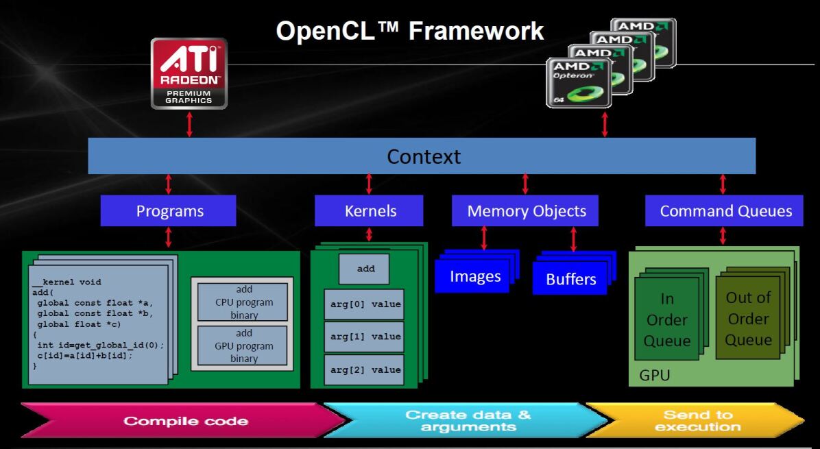
?figurename? 12.1: OpenCL Framework (from [4])

Figure 12.1 shows an overview of the OpenCL framework, taken from [4].

OpenCL defines three types of memory on GPU: global memory, local memory, and private memory. Global memory is a shared memory region on GPU, accessible to all computing units and all threads. Local memory is located on each computing device, only accessible to the computing device itself, but can be accessed much faster than global memory. Private memory is small regions of memory only accessible by each thread itself, often implemented as invidual registers on hardware. The details of memory structure is looked at in section 12.1.3, where it is shown that my algorithm fits well into this structure.

A context, roughly speaking, is a shared information structure among devices in the same platform. Data belonging to the same context can be communicated and exchanged among multiple devices, but only devices in the same platform can share the same context. For example, AMD CPUs and AMD GPUs belong to the same platform so they can share the same context, while NVIDIA GPUs belong to another platform because they use a different structure to store information, hence they cannot share the same context with AMD devices. Intel CPUs, though implemented OpenCL, have a totally different structure to any other type of devices, thus cannot share the same context with either NVIDIA device or AMD device.

A program is a piece of OpenCL code that can be compiled at run-time. OpenCL uses a subset of C99 language as fundamental programming framework, but it also allows programmers to use specific vendor extensions for optimization and debugging. For example, at present double precision floating point numbers are not officially supported by OpenCL specification. Khronos group made an extension for it, and programmers can call “#pragma OPENCL EXTENSION cl_khr_fp64 : enable” to enable this feature. AMD also have their own extension of double precision floating point numbers, which can be enabled by calling “#pragma OPENCL EXTENSION cl_amd_fp64 : enable”. More examples can be found in [6, 34].

A program can define multiple kernel functions and multiple utility functions. Kernel functions have a specific keyword “__kernel” as a signature, acting as entry points to the program to be executed on OpenCL devices. When the program compiles, OpenCL automatically optimize the program, at the same time changing all utility functions into inline functions.

A program can define constant program-wide global variables, but cannot have non-constant global variables. A program can allocate fixed size arrays, but not dynamic arrays similar to what is created by malloc() function in C. Varaibles in a program are allocated to private memory by default, but with keywords “__global” or “__local”, a variable can be allocated to device global memory or local memory, respectively.

A kernel is an entry point at execution of the program. Multiple programs and multiple kernels are allowed for the same context, but a kernel is not allowed to call another kernel in the same program, as it must be scheduled on host. Each kernel may have a set of parameters that can be allocated to private memory, local memory, or global memory. Since kernel arguments are passed from the host, it is possible to allocate a dynamic array as kernel arguments. Besides C99 primitive types, a kernel argument can also be a struct, but the struct cannot contain pointers, where the only exception when the pointers represent fixed size arrays. The reason is it does not make sense pointing to a region of memory other than fixed size arrays given OpenCL devices have their own memory management. Similarly it doesn’t make sense to have pointers as kernel arguments except when these pointers represent pre-allocated arrays.

A memory object represents a region of memory residing on the device. From the perspective of the kernel, a memory object can be read-only, write-only, or allowing both reading and writing, depending on how the memory object is created on host. Instead of residing on device, memory object can also be a pointer mapping itself to a region in host memory, if the memory object is created with flag “CL_MEM_USE_HOST_PTR”.

Each device has its own command queue to accept a sequence of command instructions from the host. Typical command instructions include launching kernel, reading memory object, writing memory object, mapping memory object to a buffer, and many others. When the host issue these commands, most of the time the programmer could choose to either block the execution of host code for synchronization or safety purposes, or not to block the execution of host code to allow more flexible and efficient scheduling. An optional notification can be sent back to the host when a command finishes execution on the kernel.

12.1.3 Hardware and Architectures

Many types of GPUs are available today, but the two major ones, NVIDIA and AMD, who use slightly different architectures, have almost all the market share in both the consumer and the professional market. Programmers need to estimate the actual memory access pattern and level of parallelism required for their applications, to find the right type of GPU which suits their purposes. A siginificant amount of analysis has been done in academia and industry to compare the performance of these two types of GPUs, unanimously reaching the same conclusion that each type of GPU has their own favourable applications. For example, long time ago in the Bitcoin community [37] people have found AMD GPUs outperform NVIDIA GPUs for everything they need, whereas in the scientific community people are often in favour to NVIDIA GPUs because of better memory effiency, greater performance in double precision computation, and better cluster energy efficiency. A comperhensive academical study comparing a modern AMD GPU and NVIDIA GPU can be found in [38].

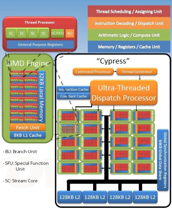
?figurename? 12.2: AMD HD5870 “Cypress” Architecture (from [5])

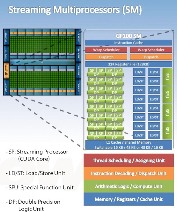
?figurename? 12.3: NVIDIA GTX480 “Fermi” Architecture (from [5])

Figure 12.2 and 12.3 shows the architecture differences between AMD GPUs and NVIDIA GPUs. This particular example compares AMD Radeon HD5870 “Cypress” GPU and NVIDIA GeForce GTX480 “Fermi” GPU. These two GPUs are released at around the same time in consumer market at approximately the same price, and they have been chosen quite often to benchmark AMD GPUs against NVIDIA GPUs for a period of time. In these figures, a warp scheduler is a thread dispatching and scheduling unit. A warp is a batch of simutaneous threads being dispatched and executed together in a Single Instruction, Multiple Data (SIMD) style. Table 4 shows their differences in a few key parameters. All processors of the Fermi GPU can operate at the shader frequency (see Table) except the schedulers and texture units.

From the table and the figures it is not hard to see that Fermi GPU has more advanced multi-thread dispatching architecture, greater core frequency, larger memory, faster memory operations, and faster memory exchange speed with host memory, benefited from its multiple dedicated scheduler units, greater memory bandwidth, and greater memory bus width. In contrast Cypress provide greater maximum computing power measured in GFLOPs, higher number of processors (cores), higher number of threads, higher number of computing devices, and better energy efficiency.

Fermi’s greater memory bandwidth is not particularly useful feature to the task at hand as long as we can keep the device busy by pushing maximum amount of data per iteration. However, in my proposed algorithm, the two-level parallelism involves considerable amount of global memory operations. Some features provided by Fermi, namely higher core frequency, higher memory frequency, and greater cache size, are greatly beneficial in this perspective. On the other hand if we could manage to reduce the amount of global memory access operations, and leverage the high throughput provided by AMD GPU to compensate its mild disadvantage in core frequency, AMD GPUs may perform much better than NVIDIA GPUs. However, achieving this may require complicated optimization at the code level for specific hardware.

GPU Name	GTX480 “Fermi”	HD5870 “Cypress”
Core Frequency	700MHz(Core) /1400MHz(Shader)	850MHz
Memory Frequency	3696MHz	1200MHz
Memory Bandwidth	177.4GB/s	153.6GB/s
Number of Cores	480	1600
Number of Computing Devices	15 Streaming Multiprocessors	20 SIMD Engines
Memory Bus width	384-bit	256-bit
GFLOPs	1345	2720
Max. Power Consumption	250W	188W

?tablename? 4: GTX480 v.s. HD5870

12.2 Implementation

Although an OpenCL kernel program must be written in C, the host program can be written in other languages. The official OpenCL specification use C++ for native host code language but wrappers have been already created for multiple languages including Java, Objective-C, Python, and many others. To achieve maximum portability without sacrifice in efficiency we have chosen Java for the implementation and the experiments. When properly implemented, Java has comparable efficiency to C and C++.

Algorithm 1 and 2 outlines the implementation pseudo code for my algorithm MGPU-DP-SPDP (Multi-GPU Distributed Parallel SPDP). As mentioned as the beginning of this section, we have transformation matrices $P^{i}$ set to identity, which limits the number of word-associations to 1, and maximum number of threads needed at topic sampling level to number of topics times 2,. Typically, two times number of topics is far less than maximum numbers of threads in a local workgroup supported by a GPU device, hence for simplicity we assume this is the case in algorithm 2, and let each thread handle exactly one probability calculation. If number of topics times 2 is more than maximum numbers of threads in a local workgroup supported by a GPU device, the only thing needs to be done is to adjust the number of probability calculations one thread is required to handle.

Readers who intend to implement the algorithm by themselves to reproduce the result should be aware that Line 22 and 24 of the pseudo code in Algorithm 2 should be computed in logarithm space to avoid overflow, especially when the required Stirling numbers can be an extremely large number at runtime. In my experiments it is observed in the original SPDP algorithm, a medium size document collection could require Stirling numbers as large as to the magnitude of $e$ to the power of hundreds or thousands. The probability formulas provided in Equation 8.17, Equation 8.18, and Algorithm 1 are proportionalities. The result must be normalized before being used to generate a sample, and appropriate technique must be used to avoid overflow. One common way is to use the identity below, where $p_{n}$ denotes the probability and $q_{n}$ denotes corresponding proportionalities: $$p_{n}=exp(\frac{\log q_{n}-\log\max\{q_{0},q_{1},q_{2},...q_{2K}\}}{\sum_{n}(\log q_{n}-\log\max\{q_{0},q_{1},q_{2},...q_{2K}\})})$$

This implementation is not optimized. The number of threads in each workgroup is not fine-tuned to suit GPU’s preference, and global memory operations are not reduced to increase its efficiency on AMD GPUs (see Section 12.1.3). An optimized implementation may further improve the running speed of my algorithm by many times, but this is not in the scope of this thesis. A basic version (which is used in the experiments) is given here to allow readers with any generic equipment able to reproduce the result.

1:Initialize OpenCL. Read data from file.

2:Randomly initialize topic assignments $z$

3:Initialize counting variables $m,n,t,q,v$ from $z$.

4:Run CPU SPDP algorithm for 1 iteration

5:Create shared device memory for common parametres

6:while Gibbs not converged do

7:     Create shared device memory $n,m,q,v$

8:     for all GPU $g$ do

9:         Create device specific memory for topic assignments $z_{g}$ from $z$, counts $t_{g}$ from $t$

10:         Create kernel with shared parameters, including device specific memory, shared device memory, and common parametres

11:         Enque execution of kernel

12:     end for

13:     Wait until all kernels have finished execution

14:     for all GPU $g$ do

15:         Read back $t_{g}$ from $g$

16:         Read back topic assignments $z_{g}$ from $g$

17:     end for

18:     Synchronize $t_{g}$ and merge into $t$

19:     Re-generate counts from $z,t$

20:end while

Algorithm 1 MGPU-DP-SPDP Host Code

1:function ParallelSampleWord(Global Counts, Shared SPDP Parametres, Local Memory Variables …)

2:     Load shared parametres into private memory

3:     $K\leftarrow$ number of topics

4:     $gid\leftarrow$ Workgroup Group ID, $lid\leftarrow$ Workgroup Local ID

5:     $d\leftarrow$ document ID, $i\leftarrow$ group ID, $w\leftarrow$ word ID of workgroup $gid$, $k\leftarrow$ topic assigned to word

6:     if $lid\leq 2K$ and $lid\equiv 0mod2$ then

7:         $kid\leftarrow lid/2$ (topic represented by $lid$)

8:         Copy global counts of topic $kid$ word $w$ group $i$ into local memory

9:         Copy global counts of topic $kid$ document $d$ group $i$ into local memory

10:         Copy auxillary global counts, e.g sums, related to topic $kid$ into local memory

11:         Correct local counts copied by $kid$ to ensure they are in valid range

12:         Correct global counts copied by $kid$ to ensure they are in valid range.

13:     end if

14:     Synchronize all threads in local workgroup

15:     if $lid\equiv 0$ then

16:         Decrement word counts in local memory in the same way as in non-parallel algorithm

17:         Decrement word counts in global memory atomically

18:     end if

19:     if $lid\leq 2K$ then

20:         $kid\leftarrow lid/2$ (topic represented by $lid$)

21:         if $lid\equiv 0mod2$ then

22:              $p[lid]\leftarrow$ probability for $z_{gid}=kid$, $r_{gid}=1$, $v_{i,k,w,t}=w$

23:         else

24:              $p[lid]\leftarrow$ probability for $z_{gid}=kid$, $r_{gid}=0$:

25:         end if

26:     else

27:         $p[lid]\leftarrow 0$

28:     end if

29:     Synchronize all threads in local workgroup

30:     if $lid\equiv 0$ then

31:         $z_{gid}\leftarrow$ new topic assignment sampled from $p$

32:         Increment counts in global memory atomically

33:     end if

34:end function

Algorithm 2 MGPU-DP-SPDP Kernel

?chaptername? 4 Experiments

13 Experimental Setup

Three datasets are used for the experiments to show the effectiveness of the three-level distributed-parallel framework introduced in Chapter 2. For all documents, words that do not carry any semantic meaning are discarded, such as “I” “you”, “she”, “he”, “are”, “is”, “it”, “am”, the so called stop words. Apostrophes, comma, and other symbols which do not carry semantic meanings are also removed, and words are tokenized into integers. We consider the plural form of a word is distinct from its singular form, as they may carry different meanings in some situations:

1. Dataset “RedState v.s DailyKos”: A blog dataset that includes 2276 blogs from American political blogs RedState (www.redstate.com) and 2386 blogs from DailyKos (www.dailykos.com) to the end of 2011. Both blogs are focused on current political issues and government policies in the United States, and related international issues, but their political positions are opposing each other. It is well known that RedState is in association with Republican politicians, and DailyKos is an active supporter of Democratic Party in the United States. I train the algorithm with 2045 and 2146 blogs from RedState and DailyKos respectively, and evaluate the perplexity on the rest of the data. After words and symbols are processed and discarded, this yields a collection of documents that has vocabulary size 14724, average effective document length of 157 words in the RedState group, and average document length of 103 words in the DailyKos group.

2. Dataset “Reuters Disaster”: A news article dataset collected from worldwide disasters news articles between 1996 to 1997, written by journalists from different regions of the news agency “Reuters”. Articles are divided into four regions: (1) Middle East and South East Asia (1508 articles), (2) European (1834 articles), (3) Asia Pacific (1580 articles), (4) America (mainly the United States, 2418 articles). For each group, 10% of the data is held out from training for computing the perplexity. After words and symbols are processed and discarded, this yields a collection of documents that has vocabulary size 51377, average effective document length of 128 words, 134 words, 132 words, and 151 words in group 1, 2, 3, 4 respectively.

3. Dataset “International Political News”: A news article dataset collected from worldwide political news sources between 1996 to 1997, containing both government releases and private news agencies. Data is divided into three groups according to location where the news article is written: (1) European and Africa (4034 articles) (2) North America and South America (5042 articles) (3) Asia Pacific (6897 articles). For each group, 10% of the data is held out from training for computing perplexity. After words and symbols are processed and discarded, this yields a collection of documents that has vocabulary size 156080, average effective document length of 184 words, 177 words, and 151 words in group 1, 2, 3 respectively.

The three datasets differ significantly in size. Dataset 1,2,3 contain about 500000, 900000, and 3000000 words respectively. In addition, the vocabulary size of dataset 2 is about 3.5 times as large as dataset 1, and the vocabulary size of dataset 3 is about 10 times as large as dataset 1.

I use the following parametres for SPDP: $\alpha=0.1$ (Dirichlet hyper-parameter for words), $\gamma=0.1$ (Dirichetlet hyper-parameter for topics), $a=0.7$ (discount parameter for SPDP), $b=100$ (concentration parameter for SPDP). These parameters are suggested as optimal parameters for blog data set by Chen [2], obtained by trial and error. It is also possible to learn the concentration parameters in the algorithm to improve the result, but these parameters are learned outside the regular collapsed Gibbs sampling cycle. Since learning these parameters is not related to the work in GPU speed improvement, these techniques are not discussed in this thesis.

Perplexity will be evaluated based on the counts after 2000 Gibbs iterations. The common practice is to run less Gibbs iterations, and to take the average output every few iterations after a burn-in period to allow the counts to enter a relatively stable region. In my experiments, this method is not used. Instead, the program runs more iterations and reads out the output only once, because longer iterations leads to better convergence, eliminates the error accumulated by taking the average output from some states that may be far away from the converging state. I observed that my improved algorithm, even when it is only running on a single GPU in my test machine, could be 50 times faster than the original SPDP implementation. When running time is no longer a concern of SPDP algorithm, there is no reason for not choosing to spend a bit more time on training in exchange for a more accurate result.

I have two machines: the first machine is a homemade GPU cluster configured with seven AMD HD5850 “Evergreen” GPUs, one AMD FX8150 “Bulldozer” CPU, and 16GB Corsair DDR III 1667MHz RAM; the second machine is a high-end laptop workstation configured with one NVIDIA GTX460M “Fermi” GPU, one Intel Core i7 740QM CPU, and 8GB Kingston 1333MHz RAM. The difference is in RAM frequency will not be an issue in benchmarking, since little computation is done on CPU, and the transmission delay between CPU and main memory is negligable. The AMD HD5850 is a reduced version of the HD5870 introduced in the last chapter, and NVIDIA GTX460M is a reduced version of the GTX480. They share the same architecture with their corresponding full versions, the differences are the number of cores, core clocks, memory rate, and memory frequency. Table 5 shows some key parameters of the four computing devices mentioned above, extracted from the vendor’s official website.

Platform	GTX460M “Fermi”	HD5850 “Cypress”	AMD FX8150 “Bulldozer”	Intel Core i7 740QM
Core Frequency	675MHz(Core) /1350MHz(Shader)	725MHz	3.6GHz~4.2GHz	1.73GHz~2.93GHz
Memory Frequency	2500MHz	1000MHz	>1866MHz	1066/1333MHz
Memory Bandwidth	60GB/s	128GB/s	N/A	N/A
Number of Cores	192	1440	8	4 (8 Threads)
GFLOPs	518.4	2088	N/A	N/A
Max. Power Consumption	50W	151W	125W	45W
Local Memory Size	48KB	32KB	N/A	N/A

?tablename? 5: Experiment Hardware Platform Comparison

Throughout the experiments, I will use the amount of time elapsed for each Gibbs iteration (minus the amount of time spent on the debugging code, such as unnecessary memory transfer between the host and the GPUs) as the measure to compare the running time of different experiments. The reason that a profiler is not used to measure the amount of time allocated to processes and kernels is that it is also desirable to to take the amount of time spent on memory operations into account. I want to measure overall how fast my algorithm is compared to the original SPDP algorithm. A fine-tuned profiler is not necessary for the task because it is expected that the running time of MGPU-SPDP is only a small fraction of the running time of the original SPDP algorithm, and we only want to get some rough ratios.

14 Experiments

The first experiment is performed on the original SPDP Java implementation. The result is used as a benchmark to compare with the results from the other experiments which are performed with different versions of MGPU-DP-SPDP that enable part or all features in the proposed three-level distributed parallelism.

Table 6 and Figure 14.1 shows the perplexity of the original SPDP algorithm with dataset “RedState v.s DailyKos” on both machines where number of topics is set to be $K=32$. The algorithm converges to approximately the same perplexity on both platforms at the same iterations, showing that although the algorithm is stochastic, the convergence speed is stable and platform independent, hence it is not necessary to test my algorithm on different devices which belong to the same class. Although the perplexity changes little after around 25 iterations, topic quality keeps getting better as the algorithm progresses, as shown in table 7. For each row in “Iterations” column, two rows in “Top Words” column corresponds to different group of documents, the first row represents RedState group, second row represents DailyKos groups. Topics are shared across groups but each group has its own ranking of a particular topic.

Platform	AMD FX8150 “Bulldozer”	Intel Core i7 740QM
Perplexity after 1 iteration	3514	3514
Perplexity after 5 iterations	2910	3028
Perplexity after 10 iterations	2449	2412
Perplexity after 25 iterations	2042	2015
Perplexity after 100 iterations	1817	1819
Perplexity after 2000 iterations	1790	1788

?tablename? 6: SPDP running time and perplexity with the dataset “RedState v.s DailyKos”

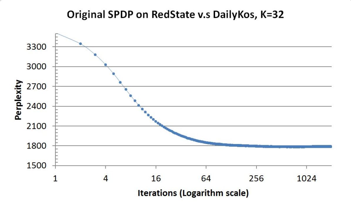
?figurename? 14.1: SPDP perplexity through Gibbs iterations (logarithm scaled) with the dataset “RedState v.s DailyKos”

Iterations	Rank	Top Words (out of top 50) in Topic 24
25	23	state, money, democrats, way, right, thing, just, california, spending, election, better, republicans, party, best, city, need, vote, really, general, left, day, second, primary, governor, republican,
	13	republicans, democrats, republican, money, election, democratic, better, need, just, thing, congress, primary, blue, majority, time, public, looking, senate, right, brown, ballot, really, state, elections
100	16	money, spending, public, democrats, want, way, good, just, big, right, problem, need, bad, important, better, budget, spend, congress, hard, time, needs, republicans, best, able, effort, trying, fund, past
	11	republicans, democrats, money, know, congress, just, democratic, republican, nation, big, better, left, got, way, time, right, trying, spending, want, year, spend, hold, need, needs, public, finally, away,
500	12	tax, taxes, spending, money, government, economic, federal, economy, business, american, year, cuts, democrats, income, congress, need, raise, spend, increase, people, jobs, policy, dollars, cut, growth
	19	money, tax, bush, economic, dollars, government, republicans, pay, spending, democrats, economy, people, iraq, run, taxes, year, corporate, time, raise, fund, federal, cut, big, recession, american,
2000	13	tax, government, taxes, economy, money, spending, economic, federal, jobs, business, increase, income, cuts, policy, year, american, growth, need, people, pay, state, cut, dollars, americans, good
	20	money, economy, tax, economic, government, dollars, bush, companies, taxes, crisis, need, spending, year, pay, american, credit, federal, america, recession, wall, increase, cut, business, social, company

?tablename? 7: SPDP topic quality progression on topic 11 with the dataset “RedState v.s DailyKos”

Table 8 shows the running time per iteration of the original SPDP algorithm with dataset “RedState v.s DailyKos” on both machines where the number of topics varies. The experiment performed on the Intel Core i7 740QM has slightly better running time due to the architectural advantage. The performance sharply dropped when the number of topics is increased to 256, due to fast expanding memory consumption (3GB) hence decreased CPU on-chip cache performance. The AMD FX8150 outperformed the Intel Core i7 740QM due to significantly larger level 2 cache (2$\times$4MB v.s. $4\times$256KB), and larger level 3 cache (8MB v.s 6MB).

Number of Topics	AMD FX8150 “Bulldozer”	Intel Core i7 740QM
32	17.700 seconds	16.510 seconds
64	35.024 seconds	32.781 seconds
128	69.746 seconds	66.230 seconds

?tablename? 8: SPDP running time for different number of topics on “RedState v.s DailyKos”

Table 9 shows the running time per iteration of original SPDP algorithm with the datasets “Reuters Disaster” and “International Political News”. Figure 14.2 and 14.3 show the perplexity convergence of the original SPDP algorithm with these two datasets. Table 10, 11, and 12 show a few converged topics of original SPDP algorithm, on the dataset “RedState v.s DailyKos”, “Reuters Disaster”, and “International Political News” respectively. The number of topics is set to 32 in these experiments.

Dataset	AMD FX8150 “Bulldozer”	Intel Core i7 740QM
“Reuters Disaster”	29.762 seconds	26.621 seconds
“International Political News”	86.355 seconds	~192 seconds (memory issue)

?tablename? 9: SPDP running time with the datasets “Reuters Disaster” and “International Political News” ($K=32$)

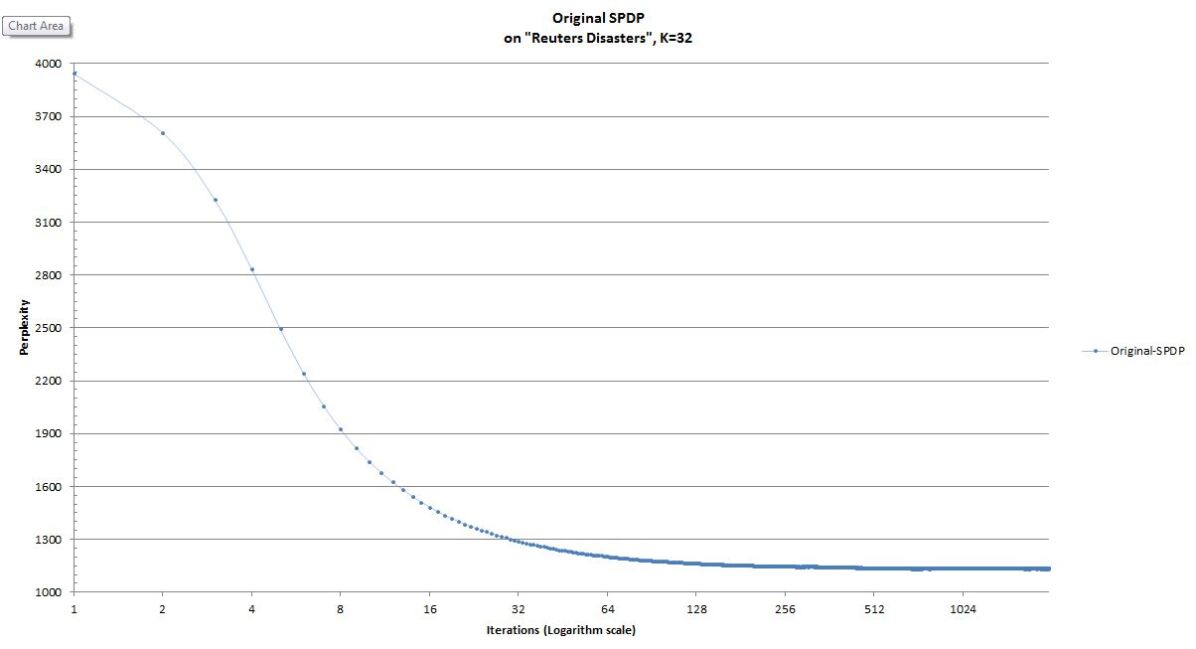
?figurename? 14.2: SPDP perplexity through Gibbs iterations (logarithm scaled) with the dataset “Reuters Disasters”

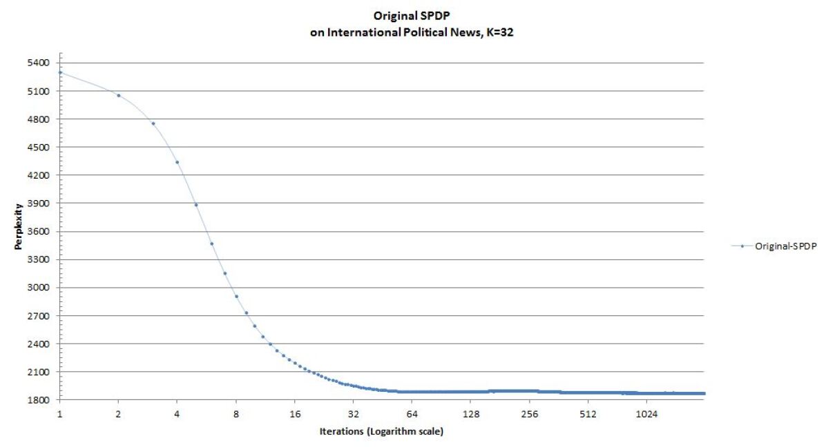
?figurename? 14.3: SPDP perplexity through Gibbs iterations (logarithm scaled) with the dataset “Reuters Disasters”

Topic ID	Probability	Rank	Top Words (out of top 50)
24	0.026321	13	tax, government, taxes, economy, money, spending, economic, federal, jobs, business, increase, income, cuts, policy, year, american, growth, need, people, pay, state, cut, dollars, americans, good
	0.017637	20	money, economy, tax, economic, government, dollars, bush, companies, taxes, crisis, need, spending, year, pay, american, credit, federal, america, recession, wall, increase, cut, business, social, company
30	0.023686	18	iraq, war, troops, surge, qaeda, iraqi, afghanistan, security, american, petraeus, military, strategy, forces, government, year, progress, general, country, withdrawal, soldiers, success, sadr, army,
	0.030925	12	iraq, war, troops, military, bush, iraqi, american, surge, years, government, americans, violence, forces, year, soldiers, iraqis, president, cheney, invasion, months, progress, plan, security, success,
31	0.042687	5	romney, huckabee, mccain, thompson, rudy, mitt, fred, campaign, iowa, candidate, republican, race, giuliani, think, john, hampshire, mike, going, candidates, debate, immigration, south, reagan, win, huck,
	0.027363	13	romney, huckabee, mccain, iowa, republican, mitt, paul, gop, poll, race, thompson, rudy, candidates, hampshire, win, mike, giuliani, republicans, fred, john, ron, candidate, campaign, voters, field, polls
16	0.013617	23	health, care, government, state, insurance, program, market, private, coverage, plan, healthcare, san, reform, city, based, mandate, medical, law, legislation, choice, pay, francisco, universal, benefits,
	0.012852	25	health, care, public, insurance, government, issues, schip, reform, flu, pandemic, times, science, children, important, coverage, ny, americans, emergency, disaster, sick, state, program, universal, safety

?tablename? 10: SPDP topic quality with dataset “RedState v.s DailyKos”

Topic ID	Probability	Rank	Top Words (out of top 50)
31	0.081832	2	iran, quake, earthquake, richter, scale, killed, iranian, irna, measuring, hit, damage, area, relief, villages, injured, official, IRAN, region, tehran, agency, province, earthquakes, news, ardabil, radio,
	0.031095	8	earthquake, scale, richter, quake, damage, tremor, iran, reported, measuring, killed, felt, town, struck, area, epicentre, eastern, institute, region, shook, gmt, injured, minor, hit, southern, miles
	0.085058	1	earthquake, scale, richter, damage, quake, measuring, tremor, region, official, reports, gmt, km, area, casualties, jiashi, miles, earthquakes, officials, china, epicentre, felt, shook, struck, seismological
	0.018930	20	earthquake, los, angeles, quake, damage, area, richter, USA, california, miles, iran, scale, reports, san, earthquakes, km, volcano, ash, struck, reported, alaska, francisco, survey, injuries, local, felt
1	0.026527	15	cyclone, state, andhra, pradesh, storm, coast, india, godavari, east, hit, coastal, officials, winds, naidu, INDIA, miles, hyderabad, rice, km, kakinada, indian, hectares, relief, port, rupees, fishermen,
	0.020554	17	poland, flood, wroclaw, floods, odra, polish, POL, water, warsaw, crisis, city, committee, opole, villages, wave, pomes, towns, sq, kwasniewski, communities, waters, czech, cimoszewicz, flooded, disaster,
	0.029046	11	mph, winds, typhoon, japan, storm, hours, shipping, expected, weather, top, southern, flooding, east, USA, north, okinawa, wsc, moving, heavy, tropical, threat, islands, sea, system, time, JAP, rains,
	0.024342	11	fire, firefighters, blaze, fires, acres, california, hectares, forest, homes, contained, san, los, burning, national, wildfires, angeles, officials, battling, burned, percent, area, miles, wildfire, malibu

?tablename? 11: SPDP topic quality with the dataset “Reuters Disasters”

Topic ID	Probability	Rank	Top Words (out of top 50)
23	0.026381	10	rights, human, report, u.n, group, international, amnesty, commission, ogoni, groups, arrested, journalists, prison, visit, abuses, statement, mission, detention, detained, nations, trial, alleged,
	0.033964	6	rights, human, china, u.n, resolution, commission, united, east, report, nations, beijing, countries, timor, international, amnesty, states, chinese, UN, torture, abuses, visit, geneva, indonesia, nigeria
	0.026651	10	rights, human, china, united, states, resolution, u.s, burma, beijing, countries, u.n, nations, visit, chinese, foreign, international, record, commission, european, asean, amnesty, world, state, year,
15	0.037233	6	vote, opposition, election, seats, results, polling, poll, percent, voting, won, assembly, voters, elections, democratic, stations, candidates, national, turnout, parties, parliament, ruling, voted,
	0.041313	5	mexico, pri, city, elections, prd, zedillo, state, pan, vote, mayor, mexican, MEX, opposition, cardenas, congress, revolutionary, electoral, institutional, ruling, election, july, revolution, democratic,
	0.033671	6	japan, ldp, hashimoto, coalition, prime, democratic, JAP, japanese, house, parliament, u.s, okinawa, lower, ministry, yen, shinshinto, liberal, tokyo, ryutaro, sakigake, parties, finance, bases, democrats

?tablename? 12: SPDP topic quality with the dataset “International Political News”

14.1 Basic Parallelization Over Topics

I implemented the proposal in Section 11.1.1, a basic parallelism over topics and word-associations (recall that only one word can be associated since the transformation matrices $P^{i}$ are identity matrices). Threads are created before Gibbs sampling initiates, and synchronized after topic and word-association probabilities are computed. This experiment is only conducted on the Intel i7 740QM CPU and the NVIDIA GTX460M GPU since the results are sufficient to show that a single level of parallelism is not efficient.

Table 13 shows the result on the dataset “RedState v.s DailyKos”. Just as we expected in Section 11.1.1, the cost of synchronization surpasses the benefit of parallelism. The original SPDP running on one thread is the consistent winner. The result shows that “easy” parallelism such as this simply does not work - it does not improve the running speed of SPDP at all.

Number of Threads	$K=32$	$K=128$
1 (CPU)	16.510 seconds	66.230 seconds
2 (CPU)	72.037 seconds	109.563 seconds
4 (CPU)	192.815 seconds	198.165 seconds
64 (CPU)	> 600 seconds	>600 seconds
$2\times K$ (GPU)	260 seconds	334 seconds

?tablename? 13: SPDP basic parallelism result with the dataset “RedState v.s DailyKos”

14.2 Parallelization Over Words

I implemented the two-level parallel proposal in Section 11.1.2. The experiments are conducted on both AMD Radeon HD5850 and NVIDIA GTX460M GPUs, with varying number of topics. This version will be refered as GPU-SPDP from now on.

Table 14 illustrates the running time of GPU-SPDP with the dataset “RedState v.s DailyKos”. Original SPDP best running times on CPU from Table 6 are provided as a single column for comparison. A massive speedup is obtained even though I did not optimize my code for the specific GPUs, as explained in Section 12.2. If the code is further optimized to device-specific parameters, we may expect a further improvement a few times better than the current result. With the implementation of Algorithm 2 only a fraction of the maximum local memory provided by both devices is used. Furthermore, the AMD HD5850, which has higher GFLOPs than the NVIDIA GTX460M, is reporting longer running time. This evidence shows that we have not used the full potential of these devices.

Table 15 shows the running time on other datasets with the number of topics set to 32. Note this is not the optimal number of topics for current implementation to get the maximum speedup.

	Running Time Per Iteration		Original	Speed Improvement
Number of Topics	GTX460M	HD5850	CPU (Fastest)	GTX460M	HD5850
32	0.518s	0.618s	16.510s	3187%	2671%
64	0.678s	0.783s	35.024s	5165%	4473%
128	1.22s	2.164s	66.230s	5429%	3060%

?tablename? 14: GPU-SPDP running time with the dataset “RedState v.s DailyKos”

	Running Time Per Iteration		Original	Speed Improvement
Dataset	GTX460M	HD5850	CPU (Fastest)	GTX460M	HD5850
Reuters Disasters	0.940s	1.146s	26.621s	2832%	2323%
International Political News	2.463	3.099s	86.355s	3506%	2787%

?tablename? 15: GPU-SPDP running time with the datasets “Reuters Disasters” and “International Political News” when $K=32$

Figure 14.4, 14.5, and 14.6 show the comparisons between the perplexity of my algorithm and the perplexity of the original algorithm for all three datasets as number of iterations progresses, when number of topics is set to 32. It can be seen from the figures that my algorithm is only slightly worse than the original algorithm in terms of perplexity. Table 16, 17, and 18 show the sample outputs of a few topics produced by the algorithm after 2000 iterations for all three datasets. From the human intepretability point of view these topics possess high quality because an ordinary human reader could understand and make sense of the words in each topic.

For example, in the result of the experiment running on dataset “RedState v.s DailyKos”:

Topic 26 shows RedState bloggers, who represent Republicans, are trying to completely avoid mentioning the issue that US government and CIA are torturing prisoners in Guantanamo detention camp who they believe are terrorists. Instead they redirect the topic to international issues in Pakistan and Israel, progress of peace negotiations in this area, and terrorism events around the globe.

Topic 22 shows bloggers from both websites are addressing the issue of global financial crisis in approximately the same fashion. The subtle difference is DailyKos bloggers are looking at the issue from the government and public point of view (as seen from words “public, matching, federal, etc.”), whereas RedState bloggers are more focused on the market itself (as seen from words “rate, credit, securities, risk, bank, (wall) street”). This is coherent to public knowledge that Democratic Party (that DailyKos represents) is running the government, and republicans are known to be close to Wall Street and big finance industry players.

Topic 4 is focused on racial and gender equality issues. RedState bloggers seem to be quite interested by the fact that Barack Obama, the current US president and leader of Democratic Party, is an African American. On the other hand DailyKos bloggers cover a range of issues in this area, treating them as equally important. The name “Ferraro” is mentioned because she is known to be a feminist who has strong opinion and great influence. She is the first female Vice Presidential candidate representing a major American political party. The city “San Francisco” is mentioned because this is the major city for racial and gender equality campaigns and protests.

Topic 12 is focused on political blogs and online media. It is very interesting that each of their website names appears as the top word in this topic.

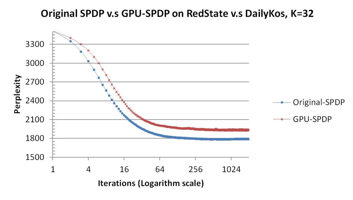
?figurename? 14.4: GPU-SPDP perplexity v.s Original SPDP with the dataset “RedState v.s DailyKos”

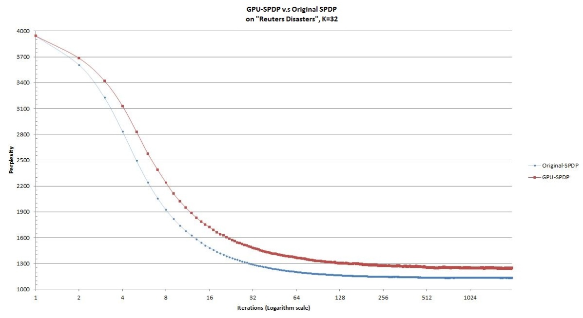
?figurename? 14.5: GPU-SPDP perplexity v.s Original SPDP with the dataset “Reuters Disasters”

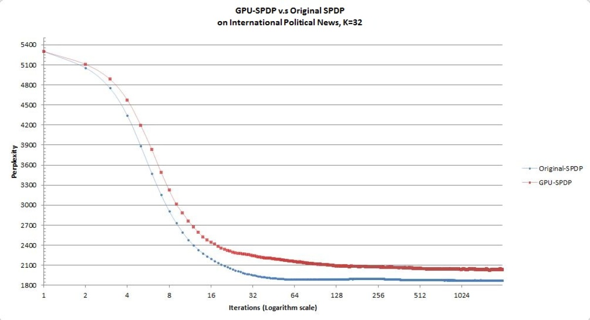
?figurename? 14.6: GPU-SPDP perplexity v.s Original SPDP with the dataset “International Political News”

Topic ID	Probability	Rank	Top Words (out of top 50)
26	0.007992	30	israel, bush, president, hamas, north, israeli, state, administration, korea, peace, rice, palestinian, terrorist, negotiations, east, knesset, talks, negotiating, enemies, annapolis, south, terrorists
	0.008642	29	torture, prisoners, tapes, cia, bush, waterboarding, guant, namo, held, tortured, evidence, destroyed, prisoner, prison, kiriakou, abu, guantanamo, perino, given, means, detainees, interrogation, gitmo
22	0.018667	12	fed, market, financial, mortgage, markets, rate, credit, money, securities, reserve, term, risk, federal, bear, bank, capital, crisis, treasury, banks, stock, value, street, short, far, rates, long, mortgages
	0.009010	28	funds, money, matching, public, federal, financing, loan, financial, bank, spending, fund, credit, mortgage, limits, spend, dollar, means, market, rate, finance, commission, complaint, cash, opinion
4	0.014814	19	barack, black, race, left, racist, rich, america, americans, african, american, chicago, king, racial, democrats, party, racism, flag, ayers, liberals, wife, jackson, san, francisco, jim, civil, rights
	0.012534	22	black, white, americans, woman, san, american, african, women, ferraro, francisco, king, racist, jackson, barack, racism, liberals, race, radio, gibson, racial, fox, civil, reilly, rights, challenge
12	0.012719	23	redstate, post, book, blog, feith, online, bloggers, read, blogs, community, readers, blogger, decision, milbank, discussion, blogging, left, writing, kos, check, moveon, posts, wing, write, sites, reading
	0.018648	13	kos, daily, bloggers, blog, progressive, media, politics, blogs, read, writers, diaries, diary, strike, writing, community, local, blogging, netroots, write, traditional, blogger, lehane, fun, kossack

?tablename? 16: GPU-SPDP topic quality with the dataset “RedState v.s DailyKos”

Topic ID	Probability	Rank	Top Words (out of top 50)
24	0.008279	30	sri, lanka, military, colombo, north, year, percent, tamil, rebels, defence, SRILAN, rupees, war, refugees, growth, northern, fighting, ltte, tigers, lankan, rebel, power, spending, jayawardena, liberation,
	0.016090	15	government, bank, flood, budget, percent, year, central, finance, zlotys, belka, relief, reconstruction, cimoszewicz, tax, loan, 2.5, credit, funds, inflation, economy, borrowing, deficit, borrow, zloty
	0.014310	23	fire, hotel, floor, building, rescue, smoke, thai, thailand, bangkok, trapped, death, broke, blaze, THAIL, top, locked, firefighters, jumped, royal, windows, toll, helicopters, started, escape, hours,
	0.018745	15	fire, firefighters, blaze, california, los, homes, angeles, san, contained, acres, winds, battling, destroyed, burned, forest, hectares, wildfire, malibu, burning, flames, diego, percent, southern,
15	0.028165	8	storm, coast, winds, cyclone, mph, hit, miles, expected, sea, east, hours, heavy, km, weather, west, meteorological, shipping, typhoon, tropical, coastal, damage, flooding, rain, month, moving, strong,
	0.006866	31	amsterdam, dakota, NETH, coastguard, north, senegal, tourists, african, sea, television, den, bodies, storm, transport, helder, tambacouda, dc-3, dakar, islands, schiphol, pleasure, national, centre,
	0.052266	4	winds, storm, mph, tropical, hurricane, typhoon, miles, expected, kph, moving, coast, north, hours, cuba, east, weather, km, forecasters, center, flooding, west, shipping, islands, USA, japan, heavy,
	0.066367	4	hurricane, storm, winds, mph, tropical, miles, north, coast, center, kph, km, forecasters, expected, west, national, moving, gmt, atlantic, florida, east, sustained, edt, warning, maximum, island, centre

?tablename? 17: GPU-SPDP topic quality with the dataset “Reuters Disasters”

Topic ID	Probability	Rank	Top Words (out of top 50)
20	0.023948	9	kabila, zaire, kinshasa, rebels, rebel, laurent, forces, capital, sese, alliance, ZAIRE, zairean, city, democratic, seko, lubumbashi, africa, kisangani, south, army, transitional, power, troops, liberation
	0.015933	17	colombia, samper, drug, colombian, COL, ernesto, extradition, campaign, bogota, la, valdivieso, serpa, carlos, farc, office, banzer, bolivia, lords, cartel, colombians, leftist, medellin, ban, charges,
	0.020348	12	deng, beijing, chinese, jiang, communist, china, xiaoping, CHINA, death, mao, li, zemin, square, power, chen, tiananmen, died, paramount, shanghai, reforms, funeral, central, army, leader, xinhua, chief,
8	0.025943	7	rights, human, commonwealth, u.n, group, international, report, britain, activists, amnesty, visit, united, abuses, countries, commission, ogoni, nations, mission, u.s, states, detainees, torture, team,
	0.035477	3	rights, human, china, u.n, resolution, commission, united, nations, east, countries, international, amnesty, report, UN, timor, states, geneva, beijing, torture, abuses, visit, foreign, indonesia, european
	0.030808	5	rights, human, china, chinese, beijing, united, tibet, resolution, u.n, states, visit, u.s, international, lama, countries, nations, dalai, commission, foreign, CHINA, record, france, world, french,

?tablename? 18: GPU-SPDP topic quality with the dataset “International Political News”

Examining the result closely, it can be noticed that some problems do exist in this version of approximation. The top topic (which is not shown here) has excessive probability in both groups, whereas the rest of the topics have much smaller probabilities compared to the result from original SPDP algorithm. This can be explained by the error accumulation due to parallel accessing same count variable through many iterations of approximation. A solution for this through word re-ordering is proposed in Section 11.1.3. In the next experiment, this is implemented in conjunction with this version of the approximation.

14.3 Effect of Re-ordering Words

As proposed in Section 11.1.3, it is expected that the amount of error can be reduced by rearranging the order of words before dispatching them to the GPU. In this experiment, this feature is added to the implementation, while everything else is as same as the previous experiment. Figure 14.7, 14.8, and 14.9 show the perplexity convergence of the improved version compared to the perplexity convergence result from GPU-SPDP and the original SPDP. Just as we did in the previous experiments, Table 19, 20, and 21 are included to show the quality of a few selected topics.

The perplexity is indeed reduced to a value almost as same as the original SPDP algorithm. The topic probabilities are in the correct range. The topic qualities are also slightly improved.

This means, now we have an algorithm which is almost as good as the original SPDP, but it runs about 30 to 50 times faster on a single consumer-grade cheap GPU which costs less than $150 USD, before any optimization, or using the power of multiple GPUs distribution framework as proposed in Section 11.2.

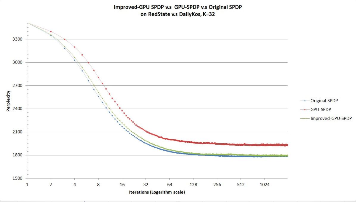
?figurename? 14.7: Improved GPU-SPDP perplexity with the dataset “RedState v.s DailyKos”

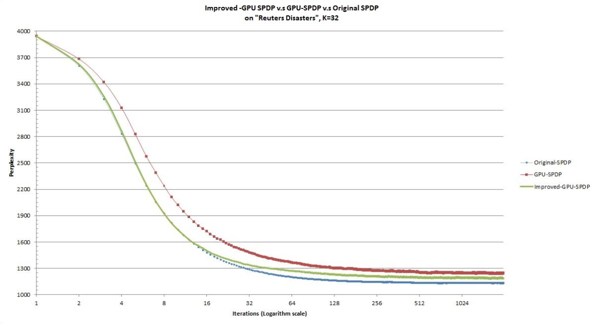
?figurename? 14.8: Improved GPU-SPDP perplexity with the dataset “RedState v.s DailyKos”

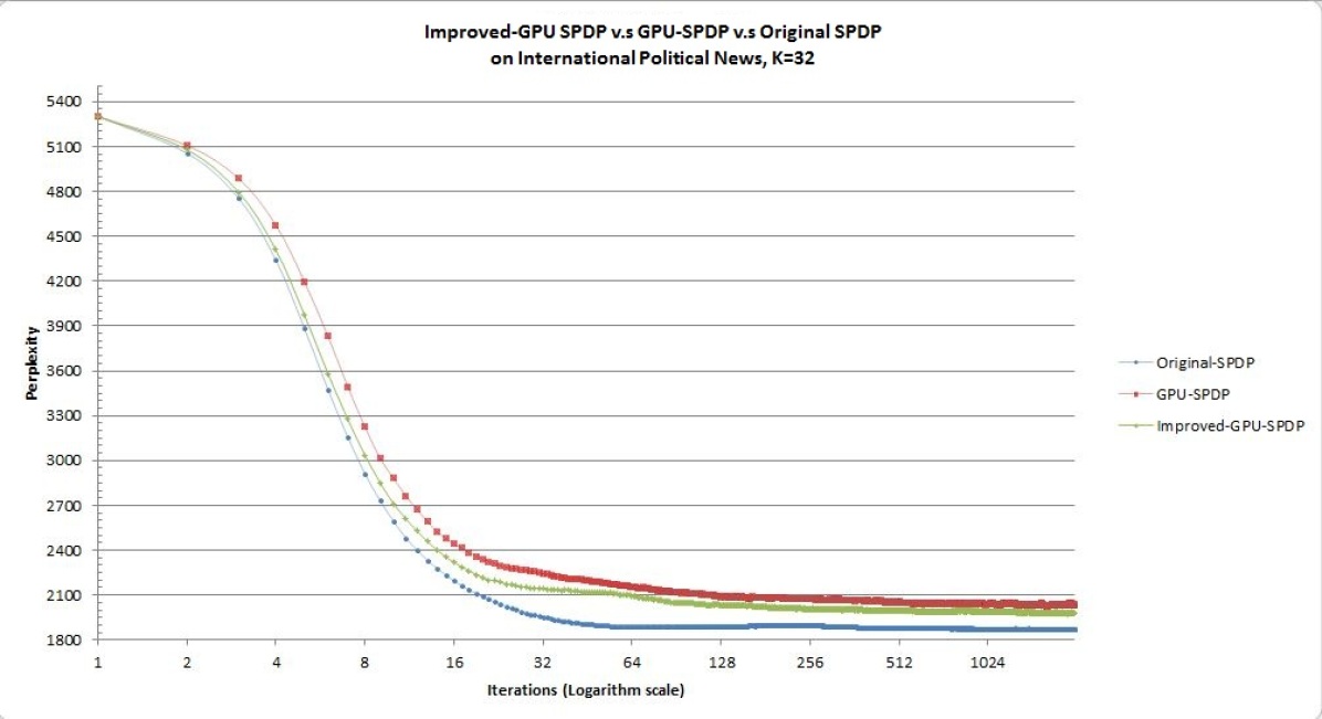
?figurename? 14.9: Improved GPU-SPDP perplexity with the dataset “RedState v.s DailyKos”

Topic ID	Probability	Rank	Top Words (out of top 50)
13	0.014364	22	campaign, money, york, corruption, paterson, murtha, foster, franken, culture, pay, democrat, party, david, office, mayor, giving, state, lobbyist, fund, wife, organizations, governor, rnc, johnson
	0.011071	30	debbie, dccc, schultz, wasserman, florida, blue, fl, chair, joe, garcia, red, trauner, south, gary, ileana, party, rahm, martinez, support, campaign, candidates, democratic, races, majority, netroots,
10	0.014269	23	senate, senator, legislation, vote, sen, committee, house, voted, floor, reid, number, democrats, mcconnell, votes, senators, passed, act, resolution, fisa, dodd, minority, read, republicans, update, mitch
	0.040049	6	senate, vote, senators, fisa, dodd, amnesty, house, republicans, senator, reid, floor, votes, update, amendment, law, democrats, filibuster, committee, telco, act, cloture, debate, retroactive, amendments
27	0.013413	15	oil, energy, global, gas, prices, food, change, production, gasoline, nuclear, warming, fuel, price, going, cost, blackhedd, climate, domestic, francis, year, companies, crude, ethanol, drive, cianfrocca
	0.019349	17	energy, global, climate, oil, warming, water, change, science, years, california, earth, gas, environment, scientists, coal, environmental, park, world, epa, action, year, land, clean, big, millions, power
18	0.024284	11	iraq, war, troops, qaeda, iraqi, military, surge, afghanistan, security, american, petraeus, general, strategy, forces, progress, soldiers, saddam, year, said, sadr, success, political, withdrawal, iraqis
	0.031108	11	iraq, war, troops, military, kristol, bush, iraqi, american, surge, americans, violence, year, government, years, soldiers, forces, afghanistan, invasion, iraqis, country, pakistan, progress, administration

?tablename? 19: Improved-GPU-SPDP topic quality with the dataset “RedState v.s DailyKos”

Topic ID	Probability	Rank	Top Words (out of top 50)
21	0.034472	9	philippines, manila, storm, PHLNS, winds, philippine, coast, miles, mph, south, expected, island, hours, sea, weather, heavy, luzon, strong, typhoon, east, north, tropical, shipping, southern, flooding,
	0.015062	24	agency, news, turkish, anatolian, TURK, quoted, istanbul, state-run, province, town, reported, crashed, southeast, fighter, dead, local, western, further, km, crashes, military, northeast, central, evening
	0.059273	4	storm, mph, winds, hurricane, tropical, expected, kph, miles, weather, hours, typhoon, coast, north, moving, km, cuba, flooding, forecasters, central, east, south, lili, center, western, islands, west,
	0.108872	2	hurricane, storm, winds, mph, tropical, miles, expected, north, coast, kph, center, hours, km, forecasters, west, moving, east, hortense, islands, national, weather, florida, flooding, shipping, gmt,
9	0.048960	6	ship, crew, vessel, port, missing, boat, cargo, sea, carrying, sank, rescued, coast, officials, ships, miles, rescue, shipping, capsized, search, members, reported, official, island, reuters, tonnes, navy
	0.058029	6	ship, port, coast, crew, sea, vessel, missing, cargo, boat, carrying, greek, island, sank, rescue, coastguard, carrier, board, officials, service, capsized, rescued, guard, aground, vessels, shipping,
	0.036614	8	ship, vessel, sheep, crew, live, port, australia, missing, sank, coast, australian, boat, trade, cargo, u.s, carrying, animal, fire, uniceb, ocean, rescued, members, search, livestock, cattle, capsized
	0.037560	6	coast, guard, u.s, crew, ship, helicopter, search, air, navy, boat, crashed, board, missing, members, marine, rescue, military, force, miles, spokesman, vessel, sea, crash, island, km, helicopters, rescued

?tablename? 20: Improved-GPU-SPDP topic quality with the dataset “Reuters Disasters”

Topic ID	Probability	Rank	Top Words (out of top 50)
12	0.013602	16	rights, human, commonwealth, u.n, group, international, nigeria, amnesty, activists, ogoni, report, abuses, groups, commission, saro-wiwa, mission, detainees, visit, team, violations, detained, nations,
	0.012239	24	u.n, taleban, rights, women, human, kabul, afghanistan, nations, nigeria, united, UN, afghan, islamic, special, mission, pakistan, visit, cambodia, military, western, north, international, masood, militia
	0.017282	14	deng, china, jiang, xiaoping, chinese, beijing, communist, death, mao, CHINA, zemin, square, died, army, paramount, economic, tiananmen, health, funeral, power, military, state, reforms, shanghai, peng,
25	0.056171	3	percent, budget, economic, year, tax, bank, finance, economy, growth, oil, industry, money, market, sector, foreign, service, policy, business, financial, deficit, spending, public, development, state,
	0.067658	2	budget, economic, tax, economy, year, bank, deficit, fiscal, spending, market, finance, growth, debt, plan, public, social, newsroom, companies, sector, cut, congress, jobs, inflation, financial, fund,
	0.073056	2	budget, tax, bank, economic, policy, economy, fiscal, growth, financial, spending, finance, cuts, business, rate, inflation, investment, market, deficit, reform, interest, sector, rates, current, industry

?tablename? 21: Improved-GPU-SPDP topic quality with the dataset “International Political News”

14.4 Multi-GPU Distributed Parallelism

Finally, I implemented the ultimate algorithm MGPU-DP-SPDP, and tested it using the same configuration as used in previous experiments except all five Radeon HD5850 GPUs on the AMD machine are used this time.

The running time analysis is shown in Table 22. For the columns representing running time of the original SPDP and GPU-SPDP, we used data from Table 14. The speed improvement over GPU-SPDP is sublinear and sometimes much lower than the maximum value (500%) because of two reasons. First, for safety reasons we used atomic locks for incrementing and decrementing variables (i.e using OpenCL primitives). For some reasons, this is necessary for AMD GPUs when multiple GPUs are used, otherwise the program would crash. We believe atomic locks are not necessary, and the result could be much more impressive if the experiment is conducted on multiple professional NVIDIA GPUs, which do not have these problems. However, we do not have the equipment at our disposal. Second, the code is not optimized, and a substantial amount of operation is wasted on memory transfer. Nonetheless, the experiment is sufficient to show that MGPU-DP-SPDP is a scalable algorithm that could improve the running speed of GPU-SPDP dramatically, sublinear to the number of GPUs available to the machine.

	Running Time Per Iteration		Original	Speed Improvement
Number of Topics	$5\times$HD5850	$1\times$HD5850	i7 740QM	To Original	To GPU-SPDP
32	0.183s	0.618s	16.510s	9022%	3377%
64	0.412s	0.783s	35.024s	8501%	1900%
128	0.95s	2.164s	66.230s	6971%	2278%

?tablename? 22: MGPU-DP-SPDP Running Time with the dataset “RedState v.s DailyKos”

	Running Time Per Iteration		Original	Speed Improvement
Datasets	$5\times$HD5850	$1\times$HD5850	CPU (Fastest)	To Original	To GPU-SPDP
Reuters Disasters	0.611s	1.146s	26.621s	4356%	187%
International Political News	1.517	3.099s	86.355s	5692%	204%

?tablename? 23: MGPU-DP-SPDP Running Time with the dataset “Reuters Disasters” and “International Political News” when $K=32$

The convergence in perplexity is shown in Figure 14.10. The perplexity is not as good as the original algorithm, but it is fairly comparable, and words for each topic still look sensible. This is because some topic probabilities are off-scale, which is discussed in the next section.

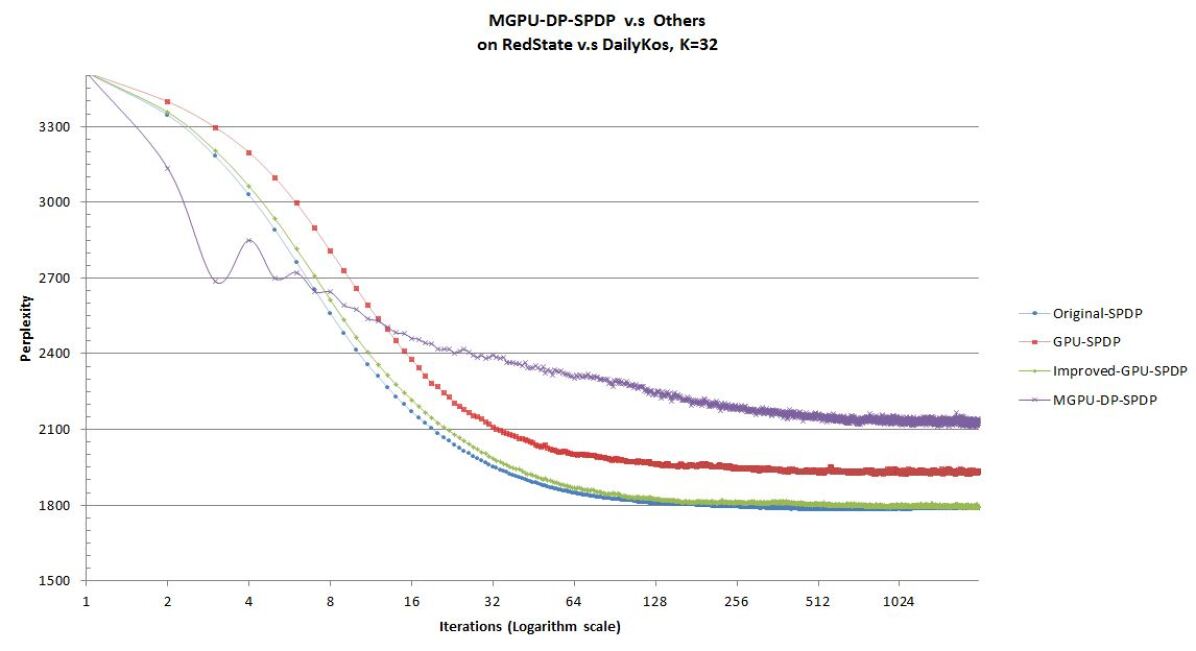
?figurename? 14.10: MGPU-DP-SPDP perplexity convergence with the dataset “RedState v.s DailyKos”

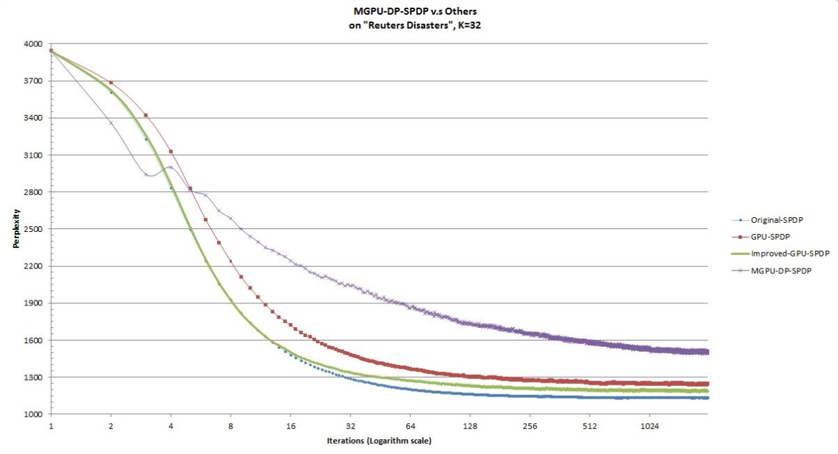
?figurename? 14.11: MGPU-DP-SPDP perplexity convergence with the dataset “Reuters Disasters”

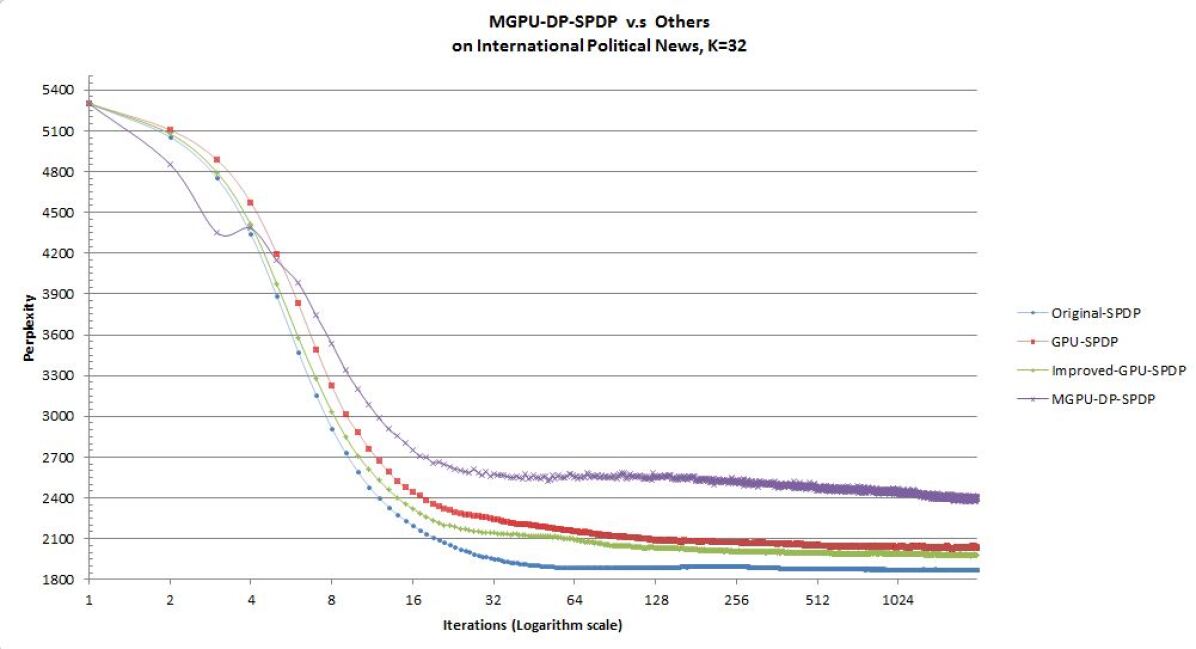
?figurename? 14.12: MGPU-DP-SPDP perplexity convergence with the dataset “International Political News”

The topic quality is shown in Table 24, 20, and 26. Occasionally strange words may appear, but overall the result is interesting, informative, and sensible.

Topic ID	Probability	Rank	Top Words (out of top 50)
21	0.009194	12	iraq, iraqi, surge, petraeus, afghanistan, military, war, sadr, forces, security, success, troops, withdrawal, baghdad, maliki, sunni, taliban, strategy, groups, anbar, counterinsurgency, shi, progress
	0.014949	7	iraq, troops, iraqi, kristol, military, war, surge, forces, violence, occupation, soldiers, invasion, iraqis, basra, success, lives, killed, cheney, sadr, security, mission, british, maliki, army, saddam,
30	0.009467	11	tax, care, taxes, insurance, health, state, private, economic, reform, federal, jobs, businesses, plan, san, costs, schwarzenegger, francisco, government, increases, revenue, taxpayers, amt, spending, city,
	0.007422	23	health, care, tax, insurance, reform, economy, taxes, coverage, cut, legislation, companies, government, state, private, bills, safety, fund, harold, programs, profit, corporations, liveblogging, plan,
19	0.007533	22	energy, oil, prices, gas, tax, gasoline, price, global, jobs, economic, cianfrocca, carbon, crude, company, companies, wheat, francis, warming, farmers, profits, costs, methanol, industrial, motor,
	0.008073	17	oil, park, epa, coal, safety, gas, global, wildlife, stickler, energy, industry, stimulus, administration, hrc, interior, environmental, plants, emissions, companies, waiver, environmentalists, economy,
22	0.008227	17	israel, iran, north, bush, israeli, world, weapons, military, palestinian, rice, nuclear, nations, foreign, president, terrorist, negotiating, peace, talks, korea, administration, knesset, borders,
	0.007767	19	bush, iran, nuclear, pakistan, bhutto, musharraf, minister, weapons, assassination, military, policy, terrorists, war, arms, blah, nato, prime, iranian, arabia, pakistani, resolution, oil, interview,

?tablename? 24: MGPU-DP-SPDP topic quality with the dataset “RedState v.s DailyKos”

Topic ID	Probability	Rank	Top Words (out of top 50)
19	0.015744	10	fire, oil, pipeline, occidental, drilling, blaze, refinery, forest, bangladesh, ongc, crude, refineries, rig, energy, assam, petroleum, ltd, sylhet, extinguish, burst, gas, bhandari, production, bazar,
	0.018931	9	fire, refinery, oil, company, plant, irish, explosion, ireland, production, leak, newsroom, gas, chemical, unit, pipeline, blaze, tonnes, rafinerska, japanese, cork, shut, illegal, trawler, a.s, hoechst,
	0.029501	3	fire, oil, refinery, plant, company, production, singapore, toyota, gas, corp, petroleum, mobil, irish, operations, taiwan, ltd, plants, leak, fishing, unit, spokesman, aisin, pipeline, taoyuan, explosion
	0.028317	4	fire, refinery, plant, oil, gas, company, unit, production, explosion, corp, pipeline, gasoline, energy, shut, tosco, barrels, bpd, crude, natural, facility, rig, drilling, texaco, units, platform, toyota
5	0.010241	19	norwegian, spitzbergen, plane, miners, longyear, arctic, mining, mountain, norway, russian, crashed, barentsburg, airliner, tu-154, NORW, land, tupolev, ntb, recorder, ukrainian, treaty, russians,
	0.009434	23	insurance, shroud, montserrat, turin, cathedral, cloth, london, blaze, caribbean, pzu, insured, claims, volcano, re, glass, cost, guarini, trematore, lloyd, christ, roman, royal, miracle, pay, image,
	0.012325	19	vietnam, insurance, storms, mekong, hanoi, claims, cambodia, rice, houses, ho, cross, delta, chi, losses, flooding, cost, year, maoming, july, compensation, zhanjiang, laos, company, picc, winbond,
	0.012907	16	earthquake, losses, authority, market, cea, insurers, insured, homeowners, claims, companies, industry, property, coverage, pay, insurance, bonds, risk, farm, butler, plan, allstate, quackenbush, premiums,

?tablename? 25: MGPU-DP-SPDP topic quality with the dataset “Reuters Disasters”

Topic ID	Probability	Rank	Top Words (out of top 50)
13	0.005928	27	burundi, hutu, buyoya, army, rebels, coup, regional, killed, ntibantunganya, frodebu, pierre, bujumbura, BURUN, talks, tanzania, imposed, embargo, cndd, tutsi, civilians, 150,000, tutsis, nyangoma, rpf,
	0.009565	17	army, rebels, rebel, epr, talks, guatemala, zapatista, guerrilla, guerrero, mexican, leftist, zapatistas, southern, marcos, guatemalan, urng, chiapas, peace, popular, zedillo, arzu, MEX, city, oaxaca,
	0.014908	5	deng, jiang, chinese, communist, xiaoping, death, mao, CHINA, zemin, square, paramount, tiananmen, shanghai, funeral, power, corruption, zedong, peng, yuan, chen, leadership, zhao, body, source, mourning
26	0.034677	3	budget, percent, economic, year, finance, tax, manuel, economy, market, sector, deficit, oil, spending, revenue, exchange, development, service, privatisation, expenditure, rate, investment, programme,
	0.033753	2	budget, tax, economic, deficit, spending, fiscal, economy, year, cut, debt, reforms, growth, measures, sector, jobs, social, newsroom, taxes, rate, bank, increase, oil, rates, fund, cuts, expected, finance,
	0.034065	2	fiscal, spending, percent, economy, policy, cuts, inflation, rates, budget, growth, rate, market, year, bank, cut, economic, reserve, deficit, savings, economists, markets, 1996/97, investment, current,

?tablename? 26: MGPU-DP-SPDP topic quality with the dataset “International Political News”

14.5 Multi-GPU Distributed Parallelism: Effect of Duplicating Training Data

It was found in one of my early implementations of MGPU-DP-SPDP (which has slightly worse error correction mechanism) that duplicating training data is sometimes crucial to get topic probabilities which do not look ridiculous. In my current version, duplicating the training data is no longer necessary. I found duplicating the data once could slightly improve the correctness of topic probabilities and the topic qualities particularly in a small document collection, which unsurprisingly results a better perplexity. Due to hardware limitations, I am unable to verify if more than one duplicate is required to improve the perplexity for a large number of GPUs, though I believe with good implementation of error correction and optimization, the need of improving the perplexity from duplicating the training data can be completely eliminated. Figure 14.13 shows the perplexity comparison after duplicating the data once for the ”RedState v.s DailyKos” dataset. Table 27 shows the topic qualities.

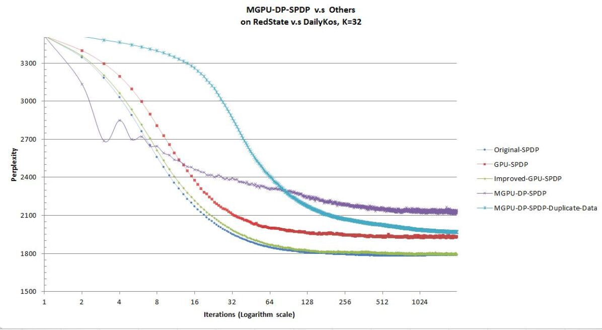
?figurename? 14.13: MGPU-DP-SPDP perplexity convergence with the duplicated dataset “RedState v.s DailyKos”

Topic ID	Probability	Rank	Top Words (out of top 50)
4	0.029230	17	trade, china, chavez, states, united, economic, policy, world, chinese, comes, russia, foreign, power, know, concerning, american, colombia, read, putin, thanks, hugo, regime, freedom, position, castro,
	0.007415	32	trade, economic, united, china, chavez, american, tremendous, know, states, policy, world, weber, nader, murray, safety, miner, neo, chinese, jones, foreign, comes, company, power, msha, canyon
30	0.023349	24	speech, human, rights, religious, religion, conservatives, jesus, liberals, faith, god, men, moral, society, constitution, question, evidence, research, certain, truth, man, merely,
	0.015697	27	religious, rights, religion, human, speech, question, faith, jesus, constitution, god, cell, stem, democracy, word, social, conservatives, church, research, progress, death, society, truth, merely, moral,
19	0.041756	6	romney, mccain, huckabee, thompson, rudy, fred, mitt, think, campaign, paul, iowa, republican, mike, john, ron, conservative, giuliani, gop, candidate, guy, going, state, said, debate, hampshire
	0.021821	21	romney, mccain, huckabee, mitt, rudy, paul, thompson, think, fred, republican, campaign, mike, gop, giuliani, iowa, john, state, going, ron, candidate, guy, candidates, conservative, said, lot, immigration
31	0.038127	10	tax, health, government, state, care, money, taxes, people, economy, private, need, spending, federal, economic, business, pay, insurance, increase, plan, market, jobs, income, program, read, americans,
	0.019285	23	health, tax, care, government, state, need, economy, people, private, pay, taxes, dollars, insurance, money, business, reform, economic, spending, federal, companies, plan, american, americans, increase,

?tablename? 27: MGPU-DP-SPDP topic quality with the duplicated dataset “RedState v.s DailyKos”

14.6 Hellinger Distance

Hellinger distance [40] is a popular measure of the similarity between two topic models. Here two heatmaps in Figure 14.14 and 14.15 are provided to show the Hellinger distance between the original SPDP and Improved-GPU-SPDP, and the Hellinger distance between the original SPDP and MGPU-DP-SPDP, both with dataset “Reuters Disasters” The x-axis is the topics as appeared in Improved-GPU-SPDP, and y-axis is the topics as appeared in the original SPDP, re-ordered to align with the topics in x-axis. Lower values mean better match in topics. The results shown here look almost as good as comparing two runs of the original SPDP.

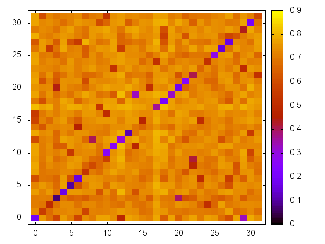
?figurename? 14.14: Hellinger distance between the original SPDP and Improved-GPU-SPDP with the dataset “Reuters Disasters”

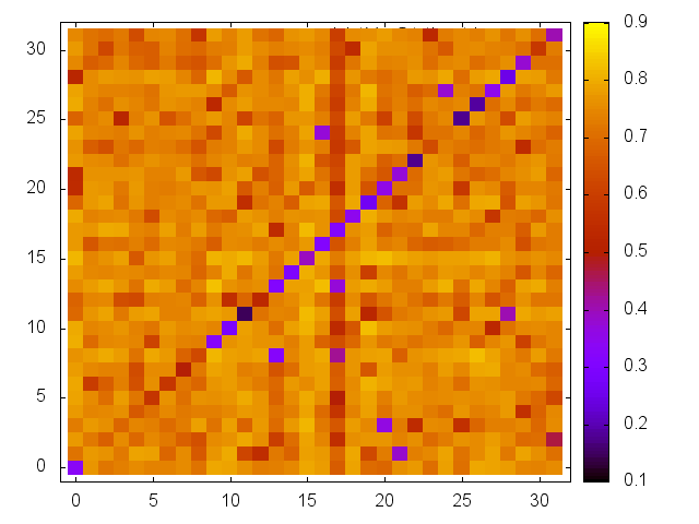
?figurename? 14.15: Hellinger distance between the original SPDP and MGPU-DP-SPDP with the dataset “Reuters Disasters”

?chaptername? 5 Conclusion

15 Conclusions and Key Contributions

I transformed the state-of-art algorithm SPDP into a distributed parallel approximation, where the running speed is substantially improved on a single GPU when only one GPU is used, and sublinearly scalable to number of GPUs available when multiple GPUs are used.

• The single GPU algorithm improved the speed of the differential topic modelling algorithm SPDP by about 50 times on a single, cheap, medium range laptop GPU.

• The multi-GPU algorithm MGPU-DP-SPDP leverages the latest modern multi-GPU architecture, improves the running speed of SPDP and topic modelling on a homemade small GPU cluster, with very small sacrifice in topic quality, and only slightly worse or fairly comparable perplexity.

• SPDP is a representative of perhaps another hundred extensions of LDA. My algorithm is designed in a generalized way, leaving mathematical derivations of SPDP intact. With little modification, the algorithm can be applied to other LDA extensions.

16 Future Work

Although the experiments have been quite successful in my experiments, there are a few other improvements that could be done:

• automated optimization tailored to GPU specifications and parameters;

• scalability and robustness of multi-GPU sampling;

• full SPDP parallelization with non-identity transformation matrices;

• large scale implementation;

• adapting the three-level distributed parallel framework to other LDA extensions.

16.1 Automated Optimization

The OpenCL framework provides APIs for users to get information about the capacity and specification of available devices. It is possible to determine the preferred local workgroup size from these information and tailor my algorithm to maximize the performance. The number of threads per workgroup should be made as close to the preferred size as possible. Each thread should be allowed to compute multiple sample probabilities, and the value should be determined by $\lceil\frac{N_{words}}{N_{threads}}\frac{K(S+1)}{T_{preferred}}\rceil$, where $N_{words}$ is the number of words that can be sampled in parallel with at most $C$ conflicts, $N_{threads}$ is the maximum number of parallel hardware threads the device supports, $K$ is number of topics, $S$ is number of word associations ($S=1$ if transformation matrix $P$ is identity), $T_{preferred}$ is the preferred local workgroup size, $C$ is a constant value to be determined. The formula simply states that we should sample as many as possible words per wave in parallel with at most $C$ conflicts. A conflict is defined as multiple access to one count variable, which could happen when two workgroups represent the same word and topic, or same word and document, or same document and topic.

To have this idea implemented efficiently, kernel code must be generated dynamically and complicated change needs to be done in host code. With this properly implemented, we may expect a significant speed improvement to the algorithm due to better occupancy hence more efficient use of GPU device.

16.2 Scalability And Robustness of Multi-GPU Sampling

The results of the experiments imply that the current error correction mechanism works well with word probabilities, but not as well with topic probabilities, hence increasing the perplexity. A better error correction mechanism is required for multi-GPU sampling. In addition, sending and reading data from multiple GPUs can be inefficient especially when the number of GPUs is large. It is possible to leave data on the GPUs, perform the error correction, random number generation, and count regeneration on GPUs. Complicated issues may arise, such as looking for an efficient way to generate random numbers and propagate to all GPU devices, and how not to make error while correcting error in parallel. We may also consider using the model introduced by Smola et al.  in [33], having a dedicated GPU to update counts for all devices. However, the implementation of this model would be very complicated, and may require approximation as some features supported by the CPU and distributed networks are not supported by the GPU and OpenCL.

16.3 Full SPDP Parallelization With Non-identity Transformation Matrices

Chen has showed in [2] that appropriate transformation matrices could uniformly improve the perplexity and the topic quality. For simplicity we implemented MGPU-DP-SPDP in Algorithm 1 and 2 assuming transformation matrices $P^{i}$ are identity matrices. As mentioned in Section 11.1.2, the difficulty in dealing with non-identity transformation matrices is in implementing a linked list $v$ that can be modified in parallel with high performance. One easy solution is to store the modifications in a separate array, which is to be merged into linked list $v$ after the GPU kernel finishes execution. However, because a massive number of words are scheduled to be sampled on the GPU, this may causes substantial delay in updating the linked list variable $v$ and the count variable $q$, which may cost the algorithm more than the benefit of non-identity transformation matrices could bring. Another approach is to allocate a fixed amount of global memory and local memory for each workgroup to store the linked list corresponding to the words they are assigned to, and merge the linked lists at the start of execution of each workgroup into the local memory. This allows any update to $v$ and $q$ to be reflected immediately, but consequently the algorithm may be slowed down substantially due to significantly increased amount of global memory access.

16.4 Large Scale Implementation

With a GPU cluster supercomputer, my algorithm has the potential to improve the running speed of SPDP and topic modelling to an unparallel level of magnitude, potentially sublinear to number of GPUs times number of cores available on a single GPU. Take this medium sized GPU cluster supercomputer [41] in CSIRO for example, a GPU cluster with 64 Tesla S2050s containing 256 GPUs with 114688 streaming processors. Assuming each GPU can only improve the running speed of SPDP by 100 times (which is a highly conservative under-estimate, consider these GPUs are all the highest range professional scientific computing GPUs, and even my cheap laptop GPU is powerful enough to improve the running speed of SPDP by 54 times before optimization). Based on the evidence in my experiments it is reasonable to estimate that my algorithm running on this GPU cluster could speed up SPDP by thousands of times before optimization, if the document collection is large enough and a few issues faced in my experiments are solved through better implmentation. This value is much greater than the speedup achieved by Smola et al$.\$did for LDA[33], which is the best speedup known so far to LDA. Of course, this is only an estimate, it may cause the algorithm to produce more error when the algorithm is running at a large scale, and it may take large amount of effort to make my algorithm scale to the level similar to CSIRO GPU cluster, since there could be many synchronization and memory issues.

16.5 Adapting the Three-level Distributed Parallel Framework to Other LDA Extensions

Although my three-level distributed parallel framework is proposed and implemented for SPDP, it does not use many specific properties of SPDP. In particular, the mathematical derivation of SPDP is not modified. This enables the algorithm to be generalized and adapted to other LDA extensions, or LDA itself. It requires few modification to the framework, and a small amount of work for implementing error correction and other related parts. The framework is especially beneficial to those extensions with complex structures with many variables. Furthermore, the same approach may be taken to parallelize and approximate Markov chains and solve a wider range of problems.

- [1] D. M. Blei, A. Y. Ng, and M. I. Jordan. Latent Dirichlet Allocation. Journal of Machine Learning Research, 3:993–1022, 2003.
- [2] Nan Ding Lexing Xie Lan Du Changyou Chen, Wray Buntine. Transformation Poisson-Dirichlet processes for differential topic modeling. In Technical report, ANU & NICTA, 2012, 2012.
- [3] Wikipedia. Zipf’s law, 2008.
- [4] Advanced Micro Devices, Inc. Heterogeneous Computing OpenCL and the ATI Radeon HD 5870 Evergreen Architecture, 2012.
- [5] Microway, Inc. GPGPU Architecture and Performance Comparison, 2010.
- [6] Advanced Micro Devices, Inc. AMD Accelerated Parallel Processing OpenCL Programming Guide, 2012.
- [7] Sungpack Hong, Tayo Oguntebi, and Kunle Olukotun. Efficient Parallel Graph Exploration on Multi-Core CPU and GPU. In Lawrence Rauchwerger and Vivek Sarkar, editors, PACT, pages 78–88. IEEE Computer Society, 2011.
- [8] Wray Buntine. Discovery in Text: Visualisation, Topics and Statistics, 2011.
- [9] Chenghua Lin and Yulan He. Joint sentiment/topic model for sentiment analysis. In Proceedings of the 18th ACM conference on Information and knowledge management, CIKM ’09, pages 375–384, New York, NY, USA, 2009. ACM.
- [10] Sang Su Lee, Tagyoung Chung, and Dennis McLeod. Dynamic Item Recommendation by Topic Modeling for Social Networks. In ITNG, pages 884–889. IEEE Computer Society, 2011.
- [11] Marco Pennacchiotti and Siva Gurumurthy. Investigating topic models for social media user recommendation. In Proceedings of the 20th international conference companion on World wide web, WWW ’11, pages 101–102, New York, NY, USA, 2011. ACM.
- [12] Noriaki Kawamae. Trend analysis model: trend consists of temporal words, topics, and timestamps. In Irwin King, Wolfgang Nejdl, and Hang Li, editors, WSDM, pages 317–326. ACM, 2011.
- [13] Arjumand Younus, Muhammad Atif Qureshi, Suneel Kumar Kingrani, et al. Investigating bias in traditional media through social media. In Alain Mille, Fabien L. Gandon, Jacques Misselis, Michael Rabinovich, and Steffen Staab, editors, WWW (Companion Volume), pages 643–644. ACM, 2012.
- [14] Michal Rosen-Zvi, Thomas Griffiths, Mark Steyvers, and Padhraic Smyth. The author-topic model for authors and documents. In Proceedings of the 20th conference on Uncertainty in artificial intelligence, UAI ’04, pages 487–494, Arlington, Virginia, United States, 2004. AUAI Press.
- [15] David Newman, Timothy Baldwin, Lawrence Cavedon, et al. Visualizing search results and document collections using topic maps. J. Web Sem., 8(2-3):169–175, 2010.
- [16] John D. Owens, Mike Houston, David Luebke, Simon Green, John E. Stone, and James C. Phillips. GPU Computing, 2009.
- [17] http://www.top500.org. Top 500 Supercomputer List, June 2012, 2009.
- [18] NVIDIA Inc. GPU’s to Crunch Data from a Square Kilometer-Sized Radio Telescope, 2011.
- [19] Bitcoin.org. Bitcoin, P2P Digital Currency, 2012.
- [20] Christopher M. Bishop. Pattern Recognition and Machine Learning. Springer, New York, 2006.
- [21] G. Heinrich. Parameter estimation for text analysis. Technical report, 2009.
- [22] Thomas Hofmann. Probabilistic Latent Semantic Analysis. In Kathryn B. Laskey and Henri Prade, editors, UAI, pages 289–296. Morgan Kaufmann, 1999.
- [23] Issei Sato and Hiroshi Nakagawa. Topic models with power-law using Pitman-Yor process. In Bharat Rao, Balaji Krishnapuram, Andrew Tomkins, and Qiang Yang, editors, KDD, pages 673–682. ACM, 2010.
- [24] Wray L. Buntine and Marcus Hutter. A Bayesian Review of the Poisson-Dirichlet Process. CoRR, abs/1007.0296, 2010.
- [25] Hemant Ishwaran and Lancelot F. James. Gibbs Sampling Methods for Stick-Breaking Priors. Journal of the American Statistical Association, 96(453):161–173, 2001.
- [26] Yee Whye Teh. A Hierarchical Bayesian Language Model Based On Pitman-Yor Processes. In Nicoletta Calzolari, Claire Cardie, and Pierre Isabelle, editors, ACL. The Association for Computer Linguistics, 2006.
- [27] Changyou Chen, Lan Du, and Wray Buntine. Sampling Table Configurations for the Hierarchical Poisson-Dirichlet Process. In Proceedings of the ECML/PKDD 2011, 2011.
- [28] Y. W. Teh, M. I. Jordan, M. J. Beal, and D. M. Blei. Hierarchical Dirichlet processes. Journal of the American Statistical Association, 101:1566–1581, 2006.
- [29] C. P. Robert and G. Casella. Monte Carlo Statistical Methods. Springer-Verlag New York Inc., 2004.
- [30] J. Pitman and M. Yor. The two-parameter Poisson-Dirichlet distribution derived from a stable subordinator. Annals of Probability, 25(2):855–900, 1997.
- [31] David Newman, Jey Han Lau, Karl Grieser, and Timothy Baldwin. Automatic Evaluation of Topic Coherence. In HLT-NAACL, pages 100–108. The Association for Computational Linguistics, 2010.
- [32] David Newman, Arthur U. Asuncion, Padhraic Smyth, and Max Welling. Distributed Algorithms for Topic Models. Journal of Machine Learning Research, 10:1801–1828, 2009.
- [33] Alexander J. Smola and Shravan Narayanamurthy. An Architecture for Parallel Topic Models. PVLDB, 3(1):703–710, 2010.
- [34] Khronos OpenCL Working Group. The OpenCL Specification, version 1.0.29, 8 December 2008.
- [35] Kamran Karimi, Neil G. Dickson, and Firas Hamze. A Performance Comparison of CUDA and OpenCL. CoRR, abs/1005.2581, 2010.
- [36] Jianbin Fang, Ana Lucia Varbanescu, and Henk J. Sips. A Comprehensive Performance Comparison of CUDA and OpenCL. In Guang R. Gao and Yu-Chee Tseng, editors, ICPP, pages 216–225. IEEE, 2011.
- [37] bitcoin.it. Mining hardware comparison, 2012.
- [38] Ying Zhang, Lu Peng, Bin Li, Jih-Kwon Peir, Jianmin Chen. Architecture Comparisons between Nvidia and ATI GPUs: Computation Parallelism and Data Communications, 2012.
- [39] D.D. Lewis, Y. Yand, T.G. Rose, and F. Li. RCV1: A New Benchmark Collection for Text Categorization Research. Journal of Machine Learning Research, 5:361–397, 2004.
- [40] Lan Du, Wray Buntine, and Huidong Jin. Modelling Sequential Text with an Adaptive Topic Model. In Empirical Methods in Natural Language Processing (EMNLP), page 9, Jeju /Korea, July 2012.
- [41] CSIRO. Speeding up science: CSIRO’s CPU-GPU supercomputer, 2012.