The $\beta$-expansion of the $D=1$ fermionic spinless Hubbard model off the half-filling regime

Abstract

We found that when the spinless model is off the half-filling regime ($\mu\neq V$), the Helmholtz free energy (HFE) can be written as two $\beta$-expansions: one expansion comes from the half-filling configuration and another one that depends on the parameter $x=\mu-V$. We show numerically that the chemical potential as a function of temperature satisfies a relation similar to the one derived from the particle-hole symmetry of the fermionic spinless model. We extend the $\beta$-expansion of the HFE of the one-dimensional fermionic spinless Hubbard model up to order $\beta^{8}$.

Key words: quantum statistical mechanics, strongly correlated electron system, spin chain models

PACS: 05.30.Fk, 71.27.+a, 75.10.Pq

Abstract

Встановлено, що для безспiнової моделi поза половинним заповненням ($\mu\neq V$) вiльну енергiю Гельмгольца можна записати у виглядi двох $\beta$-розвинень: одне розвинення походить вiд конфiгурацiї з половинним заповнення, а iнше залежить вiд параметра вiдхилення $x=\mu-V$. Чисельно показано, що хiмiчний потенцiал як функцiя температури задовольняє спiввiдношення подiбне до того, яке отримується з симетрiї частинка-дiрка фермiонної безспiнової моделi. $\beta$-розвинення вiльної енергiї Гельмгольца одновимiрної фермiонної безспiнової моделi Габбарда продовжено аж до порядку $\beta^{8}$.

Ключовi слова: квантова статистична механiка, сильно скорельвана електронна система, моделi спiнових ланцюжкiв

1 Introduction

One-dimensional models are certainly easier to handle than higher-dimensional ones, and for a long time they have been treated as toy models. In general, these models are a simplified description of a real physical system. It is often difficult to realize what is missing in those simple models in order to explain the experimental results.

The development of optical lattices over the last two decades has made possible the physical realization of one-dimensional models like the spin-$1/2$ Ising model [1], thus offering the opportunity for the experimental verification of the predictions of simplified models like the one-band Hubbard model [2, 3], that partially describes quantum magnetic phenomena.

The simplest one-dimensional fermionic model is the fermionic spinless Hubbard model, the generalizations of which have been applied to the description of Verwey metal-insulator transitions and charge-ordering phenomena of Fe₃O₄, Ti₄O₇, LiV₂O₄ and other $d$-metal compounds [4, 5, 6].

In references [7, 8] it is shown that the fermionic spinless Hubbard model in $D=1$ is mapped onto the exactly soluble $D=1$ spin-$1/2$ $XXZ$ Heisenberg model in the presence of a longitudinal magnetic field. The fermionic model has a particle-hole symmetry [8]. In reference [9] we explore the consequences of that symmetry on the thermodynamic functions of this model in the whole interval of temperature $T>0$.

The spin-$1/2$ $XXZ$ Heisenberg model is an exactly solvable model. Its thermodynamics can be derived from the thermodynamic Bethe ansatz equations [10].

Bühler et al. calculated the $\beta$-expansion of the specific heat and the susceptibility, both per site, of the frustrated and unfrustrated spin-$1/2$ Heisenberg chain up to order $\beta^{16}$ and $\beta^{24}$, respectively, in the absence of an external magnetic field [11] [$h=0$ on the r.h.s. of equation (2.2)]. In 2001 Takahashi derived an integral equation to obtain the HFE of the spin-$1/2$ $XXZ$ model [12]. The high temperature expansions of the specific heat and the susceptibility, both per site, of the isotropic spin-$1/2$ $XXX$ model [13] were calculated up to order $\beta^{100}$ also for $h=0$. In the language of the spinless model, the absence of a magnetic field in the spin-$1/2$ model corresponds to the half-filling case.

In reference [14] we calculated the $\beta$-expansion of the Helmholtz free energy (HFE) of the one-dimensional spin-$S$ $XXZ$ Heisenberg model in the presence of a longitudinal magnetic field, $S\in\{\frac{1}{2},1,\frac{3}{2},\dots$} up to order $\beta^{6}$. By applying the mapping between the aformentioned one-dimensional fermionic and spin models, we obtain the expansion of the HFE of the fermionic spinless Hubbard model also up to order $\beta^{6}$. These high temperature expansions are analytic and valid for any set of parameters of the respective Hamiltonian, thus letting one avoid the numerical solution of a hierarchy of coupled integral for every set of parameters of the spin-$1/2$ $XXZ$ model.

In the present article we study the $\beta$-expansion of thermodynamic functions of the spinless Hubbard model off the half-filling regime. We calculate two additional orders in the $\beta$-expansion of the HFE of reference [14] and verify the consequences of those extra terms on the specific heat per site and on the mean number of spinless fermions per site. We also numerically study the dependence of the chemical potential on the temperature when the number of particles in the chain is fixed.

In section 2 we present the Hamiltonian of the one-dimensional fermionic spinless Hubbard model and its mapping onto the $D=1$ spin-$1/2$ $XXZ$ Heisenberg model in the presence of a longitudinal magnetic field. We present the relations satisfied by the HFE of the model due to the particle-hole symmetry. In section 3 we discuss the $\beta$-expansion of the specific heat per site and the mean number of spinless fermions per site off the half-filling regime, and show the parameters of expansions of thermodynamic functions. In section 4 we use the $\beta$-expansion of the mean number of spinless fermions per site to numerically discuss the dependence of the chemical potential on temperature when the number of fermions in the chain is kept constant. Finally, section 5 has a summary of our results. Appendix A has the $\beta$-expansion of the HFE of the fermionic spinless Hubbard model in $D=1$, up to order $\beta^{8}$.

2 The fermionic spinless Hubbard model in $D=1$ and its exact relations

The fermionic spinless Hubbard model in $D=1$ is a very simple anti-commutative model whose Hamiltonian is [8]:

$${\bf H}(t,V,\mu)=\sum_{i=1}^{N}\;{\bf H}_{i,i+1}(t,V,\mu),$$ (2.1a)

in which

$${\bf H}_{i,i+1}(t,V,\mu)\equiv t({\bf c}_{i}^{{\dagger}}{\bf c}_{i+1}+{\bf c}_{i+1}^{{\dagger}}{\bf c}_{i})+V{\bf n}_{i}{\bf n}_{i+1}-\mu{\bf n}_{i}\,,$$ (2.1b)

the operators ${\bf c}_{i}$ and ${\bf c}_{i}^{{\dagger}}$, with $i\in\{1,2,\dots,N\}$, are the destruction and creation fermionic operators, respectively, and $N$ is the number of sites in the periodic chain (${\bf H}_{N,N+1}={\bf H}_{N,1}$). Those operators satisfy anti-commutation relations, $\{{\bf c}_{i},{\bf c}_{j}^{{\dagger}}\}=\delta_{ij}{\rm 1\hskip-2.56064ptl}_{i}$ and $\{{\bf c}_{i},{\bf c}_{j}\}=0$. In this Hamiltonian $t$ is the hopping integral, $V$ is the strength of the repulsion ($V>0$) or attraction ($V<0$) between first-neighbour fermions, and $\mu$ is the chemical potential. The operator number of fermions at the $i^{\rm th}$ site of the chain is defined as ${\bf n}_{i}\equiv{\bf c}_{i}^{{\dagger}}{\bf c}_{i}$.

It is shown in the literature [7, 8] that the equivalence of the Hamiltonian (2.1a)–(2.1b) and the one that describes the spin-$1/2$ $XXZ$ Heisenberg model in $D=1$,

$${\bf H}_{S=1/2}(J,\Delta,h)=\sum_{i=1}^{N}\left[J\left({\bf S}_{i}^{x}{\bf S}_{i+1}^{x}+{\bf S}_{i}^{y}{\bf S}_{i+1}^{y}+\Delta{\bf S}_{i}^{z}{\bf S}_{i+1}^{z}\right)-h{\bf S}_{i}^{z}\right],$$ (2.2)

in which ${\bf S}^{l}={\sigma^{l}}/{2}$, $l\in\{x,y,z\}$, and $\sigma^{l}$ are the Pauli matrices; the parameters of both Hamiltonians satisfy the relations:

$$J=2t,\qquad\Delta=\frac{V}{2t}\qquad\text{and}\qquad h=\mu-V.$$ (2.3)

The Hamiltonians (2.1a)–(2.1b) and (2.2), with their parameters satisfying conditions (2.3), differ by a constant operator

$${\bf H}(t,V,\mu)={\bf H}_{S=1/2}(J=2t,\Delta={V}/{2t},h=\mu-V)-N\left(\frac{J\Delta}{4}+\frac{h}{2}\right){\rm 1\hskip-2.56064ptl},$$ (2.4)

in which ${\rm 1\hskip-2.56064ptl}$ is the identity operator of the chain.

Let ${\cal Z}(t,V,\mu;\beta)$ and ${\cal Z}_{S=1/2}(J,\Delta,h;\beta)$ be the partition functions of the fermionic spinless model and the spin chain model, respectively,

$${\cal Z}(t,V,\mu;\beta) = \textrm{Tr}\left\{\mathrm{e}^{-\beta{\bf H}(t,V,\mu)}\right\},$$ (2.5a)

$${\cal Z}_{S=1/2}(J,\Delta,h;\beta) = \textrm{Tr}\left\{\mathrm{e}^{-\beta{\bf H}_{S=1/2}(J,\Delta,h)}\right\},$$ (2.5b)

in which $\beta={1}/{kT}$, $k$ is the Boltzmann’s constant and $T$ is the absolute temperature in kelvin.

The functions $W(t,V,\mu;\beta)$ and $W_{S=1/2}(J,\Delta,h;\beta)$ are the HFE’s associated to the Hamiltonians (2.1a)–(2.1b) and (2.2), respectively, in the thermodynamic limit ($N\rightarrow\infty$)

$$W(t,V,\mu;\beta) = -\lim_{N\rightarrow\infty}\frac{1}{N}\frac{1}{\beta}\ln\left[{\cal Z}(t,V,\mu;\beta)\right],$$ (2.6a)

$$W_{S=1/2}(J,\Delta,h;\beta) = -\lim_{N\rightarrow\infty}\frac{1}{N}\frac{1}{\beta}\ln\left[{\cal Z}_{S=1/2}(J,\Delta,h;\beta)\right],$$ (2.6b)

in which $N$ is the number of sites in the chain.

Due to the equality of operators in equation (2.4), we have a relation between the HFE’s (2.6a) and (2.6b) [8],

$$W(t,V,\mu;\beta)=W_{S=1/2}(J=2t,\Delta={V}/{2t},h=\mu-V;\beta)+\left(\frac{V}{4}-\frac{\mu}{2}\right),$$ (2.7)

valid at any non-null temperature $T$. This relation permits to relate the thermodynamic functions of both one-dimensional models.

The expression of the function $W_{S=1/2}(J,\Delta,h;\beta)$ comes from the calculation of the trace of the operator $\mathrm{e}^{-\beta{\bf H}_{S=1/2}(J,\Delta,h)}$ over all sites in the chain. In the $\beta$-expansion of this function, only terms with an even number of operators ${\bf S}_{i}^{z}$ at each site give a non-null value to the trace at the $i^{th}$ site, and, therefore, we obtain that the HFE of the one-dimensional $S=1/2$ $XXZ$ Heisenberg model is an even function of the longitudinal magnetic field $h$,

$$W_{S=1/2}(J,\Delta,-h;T)=W_{S=1/2}(J,\Delta,h;T).$$ (2.8)

Another way to understand the invariance (2.8) of $W_{S=1/2}$ is to remember the symmetry of the Hamiltonian (2.2) upon reversal of the external magnetic field, $h\rightarrow-h$, and of the spin operators, $\vec{\bf S}_{i}\rightarrow-\vec{\bf S}_{i}$, in which $i\in\{1,2,\dots N\}$.

Consider, for a given magnetic field $h$ and a fixed value (positive, null or negative) of $V$, the chemical potential $\mu$ so that $h=\mu-V$. For a reversed magnetic field, the corresponding chemical potential $\mu_{2}$ for which $-h=\mu_{2}-V$ is

$$\mu_{2}=-\mu+2V.$$ (2.9)

The identity (2.8) and the condition (2.9) recover the symmetry particle-hole of the fermionic spinless Hubbard model for any values of $V$ and $\mu$. This symmetry is summarized in the relation of the HFE of the fermionic spinless model at the same potential $V$ and different chemical potentials,

$$W(t,V,\mu;\beta)=W(t,V,\mu_{2}=-\mu+2V;\beta)-(\mu-V).$$ (2.10)

In reference [9] we explore the effect of the relation (2.10) on the thermodynamic functions of the one-dimensional fermionic spinless model at the same potential $V$ but with chemical potentials $\mu$ and $\mu_{2}$. The results discussed in reference [9] are valid in the whole range of temperatures of $T>0$.

In reference [14] we use the method of reference [15] to calculate the $\beta$-expansion of the spin-$S$ $XXZ$ Heisenberg model in $D=1$, in the presence of a longitudinal magnetic field up to order $\beta^{6}$, with $S\in\{\frac{1}{2},1,\frac{3}{2},\dots\}$ For a summary of the results of reference [15] we suggest to the reader reference [16]. Relation (2.7) permits to derive the HFE of the chain of spinless fermions from the $\beta$-expansion presented in reference [14] up to order $\beta^{6}$.

In this article we introduce a new set of rules for algebraic calculation using the method of reference [15] that enables us to calculate the $\beta$-expansion of the HFE of the fermionic spinless Hubbard model in $D=1$ up to order $\beta^{8}$.

In equation (A.1) we present the $\beta$-expansion of the HFE of the one-dimensional fermionic spinless Hubbard model up to order $\beta^{8}$. This result is calculated using the method of reference [15] for arbitrary values of the parameters in the Hamiltonian (2.1a)–(2.1b). The coefficient of the $\beta^{n}$ term, with $n\in\{-1,0,1,\dots,8\}$, in expansion (A.1) is exact. The polynomial form of the HFE expansion in $\beta$ and in the parameters of the Hamiltonian (2.1b) can be easily handled by any computer algebra system. Thermodynamic functions of the model can be derived from the appropriate derivatives of the HFE.

We explicitly verified that expansion (A.1) satisfies the relation (2.10), which is valid separately for each coefficient of the $\beta^{l}$ terms of this HFE, with $l\in\{1,2,\dots,8\}$.

3 Discussion on the $\beta$-expansion of the HFE of the model

The $\beta$-expansion (A.1) of the HFE of the fermionic spinless Hubbard model in $D=1$ permits the derivation of the $\beta$-expansion of various thermodynamic functions. In this article we discuss only two thermodynamic functions: the specific heat per site ${\cal C}(t,V,\mu;\beta)=-\beta^{2}{\partial^{2}[\beta W]}/{\partial\beta^{2}}$, and the mean number of spinless fermions per site $\rho(t,V,\mu;\beta)=-{\partial W}/{\partial\mu}$. (From this point on, it will be ommitted that those functions are calculated per site.) The expansion (A.1) is two orders higher in $\beta$ than the $\beta$-expansion of the HFE of the one-dimensional spin-$1/2$ $XXZ$ Heisenberg model, in the presence of a longitudinal magnetic field, presented in reference [14]. In what follows we make a simple comparison, the $\beta$-expansions of the specific heat and the mean number of particles, derived from the expansion of the HFE in reference [14] and equation (A.1), are compared to their respective exact expressions of two simple limiting cases, and the interval of $\beta$ in which there is a good agreement between them is determined.

In order to verify the range of convergence of each expansion, we compare them to the respective thermodynamic function of two limiting cases of the Hamiltonians (2.1a)–(2.1b) and (2.2): the free spinless fermion model [17] and the spin-$1/2$ Ising model in the presence of a longitudinal magnetic field [18]. We do not need any extra computational effort to exactly calculate these two limiting cases for arbitrary values of the parameters in their respective Hamiltonians.

Let ${\cal C}_{7}$ and ${\cal C}_{9}$ be the specific heat and the $\beta$-expansion up to order $\beta^{7}$ and $\beta^{9}$, respectively, derived from the HFE of reference [14] and equation (A.1). We have compared the expansions ${\cal C}_{7}$ and ${\cal C}_{9}$ to the specific heat of the free spinless fermion model [14] and the spin-$1/2$ Ising model [17, 18], both in $D=1$. In order to measure the difference between each specific heat of the exactly soluble models and its expansions ${\cal C}_{7}$ and ${\cal C}_{9}$, we define the percentage difference,

$$\delta_{D}{\cal C}_{k}\equiv 100\%\times\left(\frac{{\cal C}_{M}-{\cal C}_{k}}{{\cal C}_{M}}\right),\hskip 28.45274ptk\in\{7,\ 9\},$$ (3.1)

with $M\in\{\text{Ising},\ \text{Free}\}$. Let ${\cal C}_{\textrm{Ising}}$ and ${\cal C}_{\textrm{Free}}$ be the specific heat of the spin-$1/2$ Ising model and that of the free spinless fermion model, respectively.

Table 1 compares the expansions ${\cal C}_{7}$ and ${\cal C}_{9}$ to the exact specific heat of the free spinless fermion model, showing the percentage differences of the expansions of this thermodynamic function to the exact result for $t=1$, $V=0$ and $\mu=0$. Table 2 compares the exact specific heat of the spin-$1/2$ Ising model, in the presence of a longitudinal magnetic field, in $D=1$, mapped onto the fermionic spinless Hubbard model to the expansions ${\cal C}_{7}$ and ${\cal C}_{9}$ of this model, for $t=0$, $V=0.5$ and $\mu=0.8$. From data in tables 1 and 2 we conclude that the addition of two more orders in $\beta$ in the previous expansion of the specific heat increases the interval in $\beta$ where this expansion is a good approximation of the exact expression of the specific heat. Certainly, this improvement depends on the values of the set ($t,V,\mu$).

Table 1: Comparison of the percentage difference (3.1) of the expansions ${\cal C}_{7}$ and ${\cal C}_{9}$ of the specific heat of the free spinless fermion model for $t=1$, $V=0$ and $\mu=0$.

$|t|\beta$	0.5	0.82
$\delta_{D}\;{\cal C}_{7}(\%)$	– 0.35	– 7.49
$\delta_{D}\;{\cal C}_{9}(\%)$	0.04	2.38

Table 2: Comparison of the percentage difference (3.1) of the expansions ${\cal C}_{7}$ and ${\cal C}_{9}$ of the specific heat corresponding to the mapping onto the spin-$1/2$ Ising model in the presence of a longitudinal magnetic field for $t=0$, $V=0.5$ and $\mu=0.8$.

$|t|\beta$	1.6	1.91
$\delta_{D}\;{\cal C}_{7}(\%)$	– 2.10	– 6.70
$\delta_{D}\;{\cal C}_{9}(\%)$	0.54	2.32

Let $\rho_{6}(t,V,\mu;\beta)$ and $\rho_{8}(t,V,\mu;\beta)$ be the $\beta$-expansions up to order $\beta^{6}$ and $\beta^{8}$, respectively, of the average number of spinless fermions derived from the HFE of reference [14] and the equation (A.1). The effect on the convergence $\beta$-intervals due to the terms $\beta^{7}$ and $\beta^{8}$ in $\rho_{8}(t,V,\mu;\beta)$ can be determined by comparison of the expansions $\rho_{6}(t,V,\mu;\beta)$ and $\rho_{8}(t,V,\mu;\beta)$ to the exact expression of this termodynamic function on the mapping of the fermionic spinless Hubbard model onto on the spin-$1/2$ Ising model, in the presence of a longitudinal magnetic field. In analogy to (3.1), the percentage difference regarding the functions $\rho_{6}(t,V,\mu;\beta)$, $\rho_{8}(t,V,\mu;\beta)$ and $\rho_{\textrm{Ising}}$ can be defined as

$$\delta_{D}\rho_{k}\equiv 100\%\times\left(\frac{\rho_{\textrm{Ising}}-\rho_{k}}{\rho_{\textrm{Ising}}}\right),\hskip 28.45274ptk=7\;\;\mbox{or}\;\;9.$$ (3.2)

Here, $\rho_{\textrm{Ising}}$ is the mean value of the number of spinless fermions derived from the exactly soluble spin-$1/2$ Ising model.

Table 3: Comparison of the percentage difference (3.2) of the expansions $\rho_{6}$ and $\rho_{8}$ of the of the mean number of spinless fermions per site corresponding to the mapping of the fermionic spinless model onto the spin-$1/2$ Ising model in the presence of a longitudinal magnetic field for $t=0$, $V=0.5$ and $\mu=0.8$.

$\beta$	2.5	2.7	3
$\delta_{D}\;\rho_{6}(\%)$	– 0.46	– 0.78	–1.62
$\delta_{D}\;\rho_{8}(\%)$	0.35	0.67	1.64

Table 3 has been generated with the percentage difference of the expansions $\rho_{6}(t,V,\mu;\beta)$, $\rho_{8}(t,V,\mu;\beta)$ to the $\rho_{\textrm{Ising}}$, for $t=0$, $V=0.5$ and $\mu=0.8$. Data shows that for the function $\rho(t,V,\mu;\beta)$ the presence of two orders in its $\beta$-expansion does not really increase the region where the expansion is a good approximation of the exact result, although $\rho_{8}(t,V,\mu;\beta)$ is closer to the correct result.

In general, the $\beta$-expansions of the thermodynamic functions associated to a given model get worse as the parameters of the Hamiltonian increase. Let us choose two sets of values of parameters in the Hamiltonian (2.1a)–(2.1b) that map onto the spin-$1/2$ Ising model in the presence of a longitudinal magnetic field:

$$(t=0,V=0.5,\mu=0.7) \equiv (1),$$ (3.3a)

$$(t=0,V=0.5,\mu=0) \equiv (2).$$ (3.3b)

In what follows we use the notations:

$${\cal C}_{9}^{(1)} \equiv {\cal C}_{9}(t=0,V=0.5,\mu=0.7;\beta),$$ (3.4a)

$${\cal C}_{9}^{(2)} \equiv {\cal C}_{9}(t=0,V=0.5,\mu=0;\beta),$$ (3.4b)

$$\rho_{9}^{(1)} \equiv \rho_{9}(t=0,V=0.5,\mu=0.7;\beta),$$ (3.4c)

$$\rho_{9}^{(2)} \equiv \rho_{9}(t=0,V=0.5,\mu=0;\beta).$$ (3.4d)

Figure 1 show the percentage differences of ${\cal C}_{9}$ and $\rho_{9}$, given by (3.1) and (3.2), respectively, to their respective exact expressions for the set of values (3.3a) and (3.3b). Figure 1 show that for both thermodynamic functions the percentage differences increase more rapidly for $\mu=0$ than for $\mu=0.7$. How to explain that a higher value of $\mu$ yields a larger interval in $\beta$ where the expansions of the thermodynamic functions are better approximations of the exact functions?

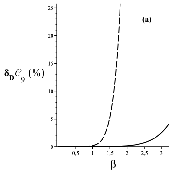
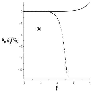
Figure 1: (a): percentage differences of ${\cal C}_{9}^{(1)}$ (solid line) and ${\cal C}_{9}^{(2)}$ (dashed line) to the specific heat of the spin-$1/2$ Ising model. (b): percentage differences of $\rho_{9}^{(1)}$ (solid line) and $\rho_{9}^{(2)}$ (dashed line) to the mean value of spinless fermions also derived from the spin-$1/2$ Ising model.

In order to understand the convergence behavior of the expansions of the functions ${\cal C}(t,V,\mu;\beta)$ and $\rho(t,V,\mu;\beta)$, we define the parameter

$$x\equiv\mu-V=h.$$ (3.5)

as a measure of how much the chain is off the half-filling regime (i.e., $\mu=V$). Rewriting the relation (2.7) between the HFE’s of the one-dimensional fermionic spinless Hubbard model and the spin-$1/2$ $XXZ$ Heisenberg model in $D=1$ in the presence of a longitudinal magnetic field in terms of the parameter $x$, we obtain

$$W(t,V,\mu=V+x;\beta)=-\left(\frac{V}{4}+\frac{x}{2}\right)+W_{S=1/2}\left(J=2t,\Delta={V}/{2t},h=x;\beta\right).$$ (3.6)

The function $W_{S=1/2}(J,\Delta,h;\beta)$ has a Taylor expansion in $\beta$ whose coefficient of the $\beta^{n}$ term is a product of powers of the parameters in Hamiltonian (2.2), $J^{n_{1}}\Delta^{n_{2}}h^{n_{3}}$, with $n_{1}+n_{2}+n_{3}=n+1$. This thermodynamic function can be written as an expansion in any of the parameters: $J,\Delta,h$ and $\beta$. The expansion of $W_{S=1/2}$ around $h=0=x$ corresponds to an expansion of $W(t,V,\mu=V+x;\beta)$ about the half-filling configuration, $\mu=V$.

Expanding the HFE $W(t,V,\mu=V+x;\beta)$ about $x=0$ yields

$$W(t,V,\mu=V+x;\beta)\equiv W(t,V,\mu=V;\beta)+\widetilde{W}(t,V,x;\beta),$$ (3.7a)

in which

$$\widetilde{W}(t,V,x=0;\beta)=0.$$ (3.7b)

The symmetry relation (2.8) and the definition (3.7a) permit to conclude that

$$\widetilde{W}(t,V,x;\beta)=-\frac{x}{2}+\omega(t,V,x^{2};\beta).$$ (3.8)

From the form the HFE in equation (3.7a) is written, one can affirm that the thermodynamic quantities of the chain off the half-filling regime can be expressed as a contribution of the half-filling configuration plus an amount due to how off the system is from the half-filling regime (that depends, naturally, on the parameter $x$).

The decomposition (3.7a) and the definitions of the specific heat and the mean number of fermions permit us to write those functions in terms of the parameter $x$,

$${\cal C}(t,V,\mu=V+x;\beta)={\cal C}(t,V,\mu=V;\beta)+\Delta{\cal C}(t,V,x;\beta),$$ (3.9a)

in which

$$\Delta{\cal C}(t,V,x;\beta)\equiv-\beta^{2}\;\frac{\partial^{2}[\beta\widetilde{W}(t,V,x;\beta)]}{\partial\beta^{2}},$$ (3.9b)

and

$$\rho(t,V,\mu=V+x;\beta)=\frac{1}{2}+\Delta\rho(t,V,x;\beta)$$ (3.10a)

with

$$\Delta\rho(t,V,x;\beta)\equiv-\frac{\partial}{\partial x}\left[\widetilde{W}(t,V,x;\beta)+\frac{x}{2}\right].$$ (3.10b)

Returning to the set of values (3.3a) and (3.3b) for the parameters of Hamiltonian (2.1a)–(2.1b) we notice that the values of $x$ for those sets are, respectively,

$$x^{(1)}=0.2\qquad\text{and}\qquad x^{(2)}=-0.5.$$ (3.11)

Notice that the absolute value of $x^{(1)}$ is smaller than the absolute value of $x^{(2)}$, and this explains why the good approximations of those two functions are obtained in intervals of $\beta$ that are larger for the set (3.3a) than those for the set (3.3b). This result is clearly shown in figure 1.

In order to verify that $x$ is one of the possible parameters of an expansion of the function $\rho(T,V,\mu=V+x;\beta)$ rather than the chemical potential $\mu$, we calculate the percentage weight of the $\beta^{8}$ term in its $\beta$-expansion. Let us denote the $\beta$-expansion of $\Delta\rho$ by

$$\Delta\rho_{8}(t,V,x;\beta)\equiv\sum_{l=1}^{8}\;a_{l}(t,V,x)\;\beta^{l}.$$ (3.12)

The percentage weight $\delta_{W}a_{8}$ of the $\beta^{8}$ term in the expansion of $\Delta\rho$ is

$$\delta_{W}a_{8}(t,V,x;\beta)\equiv 100\%\;\frac{a_{8}(t,V,x)\beta^{8}}{\Delta\rho(t,V,x;\beta)}.$$ (3.13)

Table 4: The values of $|t|\beta_{\textrm{max}}$ calculated from the percentage weight $\delta a_{8}$ (3.13) for $t=1$ and ${V}/{|t|}=0.5$.

$\frac{x}{|t|}$	$\frac{\mu}{|t|}$	$|t|\beta_{\textrm{max}}$	$\delta_{W}\;a_{8}(\%)$
$\pm$ 0.1	0.4	1.12	– 4.13
	0.6
$\pm 0.5$	0	0.98	+ 4.03
	1
$\pm 1$	– 0.5	0.77	+ 4.03
	1.5

Let $\beta_{\textrm{max}}$ be the maximum value of the variable $\beta$ for which $|\delta_{W}a_{8}(t,V,x;\beta)|\stackrel{{\scriptstyle<}}{{{}_{\sim}}}4\%$, and for which we expect that the expansion should be still a good approximation to the exact function $\Delta\rho(t,V,x;\beta)$. Table 4 shows the values of $|t|\beta_{\textrm{max}}$ and the corresponding value of $\delta_{W}a_{8}$ for different values of ${x}/{|t|}$ for $t=1$ and ${V}/{|t|}=0.5$. The second column in this table shows the two distinct values of $\mu$ for which the same value of $|t|\beta_{\textrm{max}}$ is obtained. In particular, for ${x}/{|t|}=\pm 0.5$ we have the chemical potentials $\mu=0$ and $\mu=1$ yielding the same value of $|t|\beta_{\textrm{max}}$.

In order to discuss the value of $\beta_{\textrm{max}}$ for which the specific heat can be well described by its expansion, we define the coefficients of the $\beta$-expansions of ${\cal C}(t,V,\mu=V+x;\beta)$ and of the function $\Delta{\cal C}(t,V,x;\beta)$,

$${\cal C}_{9}(t,V,\mu=V+x;\beta)\equiv\sum_{l=2}^{9}\;\;c_{l}(t,V,x)\beta^{l}$$ (3.14a)

and

$$\Delta{\cal C}_{9}(t,V,x;\beta)\equiv\sum_{l=2}^{9}\;\;g_{l}(t,V,x)\beta^{l}.$$ (3.14b)

We also define the percentage weight $\delta_{W}c_{9}$ of the term of order $\beta^{9}$ in the expansion ${\cal C}_{9}$ as

$${\delta_{W}c_{9}}(t,V,x;\beta)\equiv 100\%\;\frac{c_{9}(t,V,x)\beta^{9}}{{\cal C}_{9}(t,V,V+x;\beta)},$$ (3.15)

in order to determine the value of $\beta_{\textrm{max}}$ for the specific heat.

Table 5: The percentage weight $\delta_{W}c_{9}$ of the term of order $\beta^{9}$ in the expansion ${\cal C}_{9}(t,V,V+x;\beta)$. The values of $|t|\beta_{\textrm{max}}$ are calculated for $t=1$ and ${V}/{|t|}=0.5$.

$\frac{x}{|t|}$	$\frac{\mu}{|t|}$	$|t|\beta_{\textrm{max}}$	$\delta_{W}\;c_{9}(\%)$
$\pm$ 0.1	0.4	0.68	– 4.10
	0.6
$\pm 0.5$	0	0.69	– 4.06
	1
$\pm 1$	– 0.5	0.65	+ 4.05
	1.5

Table 5 shows the values of $|t|\beta_{\textrm{max}}$ for the specific heat where $\delta_{W}c_{9}\stackrel{{\scriptstyle<}}{{{}_{\sim}}}4\%$. The calculations have been done with $t=1$ and ${V}/{|t|}=0.5$. Again we obtain that for $x=\pm 0.5$, the $\beta$- interval, where the expansion ${\cal C}_{9}$ is a good approximation of the exact expression of this thermodynamic function, is the same for $\mu=0$ and $\mu=1$.

The function $\Delta{\cal C}$ in equation (3.9b) measures the difference between the specific heat in the half-filling regime and that function at the chemical potential $\mu=V+x$. It also has a $\beta$-expansion that depends on $x$. In order to verify the value of $\beta_{\textrm{max}}$ for the function $\Delta{\cal C}_{9}$, we define the percentage weight of the term of order $\beta^{9}$ in this function,

$$\delta_{W}g_{9}(t,V,x;\beta)\equiv 100\%\;\frac{g_{9}(t,V,x)\beta^{9}}{\Delta{\cal C}_{9}(t,V,x;\beta)}.$$ (3.16)

Table 6 shows the values of $|t|\beta_{\textrm{max}}$ for the function $\Delta{\cal C}_{9}(t,V,x;\beta)$ with $|t|=1$ and ${V}/{|t|}=0.5$. We verify that the values of $|t|\beta_{\textrm{max}}$ for the functions ${\cal C}_{9}(t,V,V+x;\beta)$ and $\Delta{\cal C}_{9}(t,V,x;\beta)$ can be different.

Table 6: The percentage weight $\delta_{W}g_{9}(\%)$ of the term of order $\beta^{9}$ in the expansion of $\Delta{\cal C}_{9}(t,V,V+x;\beta)$. The values of $|t|\beta_{\textrm{max}}$ are calculated for $t=1$ and ${V}/{|t|}=0.5$.

$\frac{x}{|t|}$	$\frac{\mu}{|t|}$	$|t|\beta_{\textrm{max}}$	$\delta_{W}g_{9}(\%)$
$\pm$ 0.1	0.4	0.56	– 4.03
	0.6
$\pm 0.5$	0	0.56	+ 4.05
	1
$\pm 1$	– 0.5	0.47	+ 4.00
	1.5

4 The temperature dependence of the chemical potential

The chemical potential $\mu$ is one of the parameters in the Hamiltonian (2.1a)–(2.1b). For a given fixed value of $\mu$, the relation $\rho(t,V,\mu;\beta)=-{\partial W(t,V,\mu;\beta)}/{\partial\mu}$ permits the determination, from the expansion (A.1), how the mean number of spinless fermions varies with the temperature.

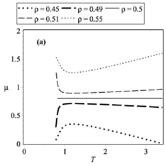
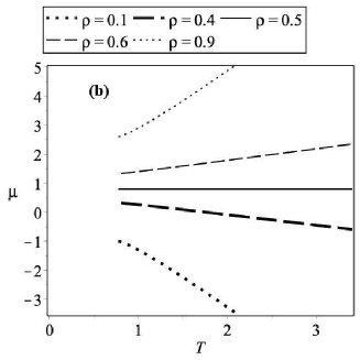
Figure 2: The chemical potential $\mu(t,V,\rho_{8};T)$ as function of the temperature $T$. (a): for $t=1$ and ${V}/{|t|}=0.8$. (b): for $t=0$ and ${V}/{|t|}=1$.

How should the chemical potential vary for a given temperature $T$, keeping the chain in thermal equilibrium at this temperature, so that the chain keeps its number of fermions per site? The relation between $\rho(t,V,\mu;\beta)$ and $W(t,V,\mu;\beta)$ permits to rewrite the expansion $\rho_{8}(t,V,\mu;\beta)$ as a polynomial in the chemical potential $\mu$ of order $\mu^{7}$, written as

$$\rho_{8}=n_{0}(t,V;\beta)\mu^{0}+n_{1}(t,V;\beta)\mu^{1}+\cdots+n_{7}(t,V;\beta)\mu^{7}.$$ (4.1)

The coefficients $n_{l}(t,V;\beta)$, with $l\in\{0,1,\dots,7\}$, are known and — differently from the coefficients of the $\beta$-terms in the expansion (A.1) — they have corrections from higher orders in $\beta$.

In order to derive the dependence of the function $\mu$ on the variables $\rho_{8}$, $t,V$ and $\beta$, one must obtain the roots of a $7^{\rm th}$ degree polynomial in $\mu$. Figure 2 show our numerical results for the dependence of $\mu$ on the temperature $T$ for $t=0$ and $t=1$, for fixed values of ${V}/{|t|}$ and $\rho_{8}$.

By comparing the curves in each graph of figure 2, we obtain the relation

$$\mu(t,V,\rho=0.5+\delta;T)=2V-\mu(t,V,\rho=0.5-\delta;\beta),$$ (4.2)

with $\delta\in[-0.5,0.5]$. This is similar to equation (2.9), derived from the hole-particle symmetry of the one-dimensional fermionic spinless Hubbard model.

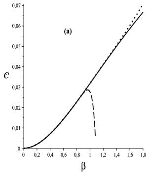
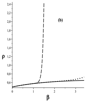
Figure 3: (a): comparison of the specific heat curves ${\cal C}_{\textrm{Ising}}$ (solid line), ${\cal C}_{8}$ (dotted line) and ${\cal C}_{24}$ (dashed line). (b): comparison of the average number of fermions $\rho_{\textrm{Ising}}$ (solid line), $\rho_{7}$ (dotted line) and $\rho_{23}$ (dashed line). In both panels, $t=0$, $V=0.5$ and $\mu=0.9$.

5 Conclusions

The one-dimensional fermionic spinless fermionic Hubbard model is the simplest fermionic model, and it has the particle-hole symmetry. This model can be mapped onto the spin-$1/2$ $XXZ$ Heisenberg model in the presence of a longitudinal magnetic field in $D=1$. Some years ago we derived the $\beta$-expansion of the HFE of the latter up to order $\beta^{6}$ [14]. In this article we have extended the $\beta$-expansion of the HFE of both models up to order $\beta^{8}$. Each $\beta$ term in the expansion satisfies the condition (2.10) derived from the particle-hole symmetry of the one-dimensional fermionic model.

We have used the expansion (A.1) of the HFE of the fermionic spinless model (2.1a)–(2.1b) to study how the interval of convergence (in $\beta$) of the specific heat per site [${\cal C}(t,V,\mu;\beta)$] and of the mean number of spinless fermions per site [$\rho(t,V,\mu;\beta)$] is modified by the presence of two more orders in $\beta$ in their respective expansions.

An interesting result that we obtain for the $\beta$ expansions of the thermodynamic functions comes from the relation (2.7) between the HFE of the fermionic spinless model and the spin-$1/2$ model. When the chain is off the half-filling regime ($\mu\not=V$), the relation (2.7) permits to write the thermodynamic functions of the chain in this regime as two $\beta$-expansions: the expansion of the function in the half-filling ($\mu=V$) plus another expansion that depends on the set of parameters ($t,V,x=\mu-V;\beta)$. The parameter $x$ is a measure of how off the chain is from the half-filling regime. This fact explains why the expansions ${\cal C}_{9}(t,V,\mu;\beta)$ and $\rho_{8}(t,V,\mu;\beta)$ with $\mu=0$ have shorter $\beta$ intervals of convergence than those for $|\mu|>0$.

We have numerically obtained the dependence of the chemical potential $\mu$ on the temperature $T$ when the mean value of fermions per site $\rho$ is kept fixed. We have verified that the relation (4.2), satisfied by $\mu(T)$ for $\rho=0.5\pm\delta$ with $\delta\in[-0.5,+0.5]$, is similar to equation (2.9) derived from the particle-hole symmetry of the fermionic spinless Hubbard model in $D=1$.

Finally, we point out that the present $\beta$-expansion of the HFE of the one-dimensional spinless Hubbard model is valid for any set of parameters of its Hamiltonian, including the cases $V>0$ (repulsion) and $V<0$ (attraction).

Appendix A The HFE of the one-dimensional fermionic spinless Hubbard model up to order $\beta^{8}$

We have applied the method of reference [15] to calculate the $\beta$-expansion of the HFE associated to the Hamiltonian (2.1a)–(2.1b) and to the Hamiltonian (2.2) [see equation (2.7)]. We have also implemented a new set of rules that permit the algebraic computation of the HFE of the one-dimensional fermionic spinless Hubbard model up to order $\beta^{8}$,

$$W(t,V,\mu;\beta)=\!\! - \frac{\ln\left(2\right)}{\beta}+\frac{1}{4}\,V-\frac{1}{2}\,\mu+\left(-\frac{5}{32}\,{V}^{2}+1/4\,V\mu\frac{1}{8}\,{\mu}^{2}-\frac{1}{4}\,{t}^{2}\right)\beta$$ (A.1)

$$+ \left(\frac{1}{16}\,{V}^{3}-\frac{1}{8}\,{V}^{2}\mu+\frac{1}{16}\,V{\mu}^{2}-\frac{1}{16}\,V{t}^{2}\right){\beta}^{2}+\left(-\frac{31}{3072}\,{V}^{4}+\frac{1}{96}\,{V}^{3}\mu+\frac{1}{64}\,{V}^{2}{\mu}^{2}\right.$$

$$+ \left.\frac{7}{96}\,{V}^{2}{t}^{2}-\frac{1}{48}\,V{\mu}^{3}-1/8\,V\mu\,{t}^{2}+\frac{1}{192}\,{\mu}^{4}+\frac{1}{16}\,{\mu}^{2}{t}^{2}+\frac{1}{32}\,{t}^{4}\right){\beta}^{3}+\left(-{\frac{1}{128}}\,{V}^{5}\right.$$

$$+ {\frac{7}{192}}\,{V}^{4}\mu-{\frac{23}{384}}\,{V}^{3}{\mu}^{2}-{\frac{7}{256}}\,{V}^{3}{t}^{2}+\frac{1}{24}\,{V}^{2}{\mu}^{3}+\frac{1}{16}\,{V}^{2}\mu\,{t}^{2}-{\frac{1}{96}}\,V{\mu}^{4}-\frac{1}{32}\,V{\mu}^{2}{t}^{2}$$

$$+ \left.\frac{1}{32}\,V{t}^{4}\right){\beta}^{4}+\left({\frac{287}{36864}}\,{V}^{6}-{\frac{239}{7680}}\,{V}^{5}\mu+{\frac{139}{3072}}\,{V}^{4}{\mu}^{2}\right.-{\frac{21}{2560}}\,{V}^{4}{t}^{2}-{\frac{31}{1152}}\,{V}^{3}{\mu}^{3}$$

$$+ {\frac{7}{192}}\,{V}^{3}\mu\,{t}^{2}+{\frac{5}{1536}}\,{V}^{2}{\mu}^{4}-{\frac{23}{384}}\,{V}^{2}{\mu}^{2}{t}^{2}-{\frac{47}{1536}}\,{V}^{2}{t}^{4}+{\frac{1}{480}}\,V{\mu}^{5}+\frac{1}{24}\,V{\mu}^{3}{t}^{2}$$

$$+ \frac{1}{16}\,V\mu\,{t}^{4}-{\frac{1}{2880}}\,{\mu}^{6}\left.-{\frac{1}{96}}\,{\mu}^{4}{t}^{2}-\frac{1}{32}\,{\mu}^{2}{t}^{4}-{\frac{1}{144}}\,{t}^{6}\right){\beta}^{5}+\left(-{\frac{29}{10240}}\,{V}^{7}\right.$$

$$+ {\frac{389}{46080}}\,{V}^{6}\mu-{\frac{119}{30720}}\,{V}^{5}{\mu}^{2}+{\frac{1603}{92160}}\,{V}^{5}{t}^{2}-{\frac{7}{576}}\,{V}^{4}{\mu}^{3}-{\frac{53}{768}}\,{V}^{4}\mu\,{t}^{2}+{\frac{41}{2304}}\,{V}^{3}{\mu}^{4}$$

$$+ {\frac{157}{1536}}\,{V}^{3}{\mu}^{2}{t}^{2}+{\frac{83}{23040}}\,{V}^{3}{t}^{4}-{\frac{17}{1920}}\,{V}^{2}{\mu}^{5}-{\frac{13}{192}}\,{V}^{2}{\mu}^{3}{t}^{2}-{\frac{1}{64}}\,{V}^{2}\mu\,{t}^{4}+{\frac{17}{11520}}\,V{\mu}^{6}$$

$$+ {\frac{13}{768}}\,V{\mu}^{4}{t}^{2}+{\frac{1}{128}}\,V{\mu}^{2}{t}^{4}\left.-{\frac{11}{768}}\,V{t}^{6}\right){\beta}^{6}+\left(-{\frac{108527}{165150720}}\,{V}^{8}+{\frac{17}{645120}}\,{\mu}^{8}\right.$$

$$+ {\frac{17}{9216}}\,{t}^{8}+{\frac{1709}{46080}}\,{V}^{5}\mu\,{t}^{2}-{\frac{1439}{30720}}\,{V}^{4}{\mu}^{2}{t}^{2}+{\frac{19}{1152}}\,{V}^{3}{\mu}^{3}{t}^{2}-{\frac{83}{1536}}\,{V}^{3}\mu\,{t}^{4}$$

$$+ {\frac{49}{4608}}\,{V}^{2}{\mu}^{4}{t}^{2}+{\frac{73}{1024}}\,{V}^{2}{\mu}^{2}{t}^{4}-{\frac{17}{1920}}\,V{\mu}^{5}{t}^{2}-{\frac{17}{384}}\,V{\mu}^{3}{t}^{4}-{\frac{17}{576}}\,V\mu\,{t}^{6}$$

$$+ {\frac{9241}{1290240}}\,{V}^{7}\mu-{\frac{8939}{368640}}\,{V}^{6}{\mu}^{2}-{\frac{12877}{1290240}}\,{V}^{6}{t}^{2}+{\frac{3539}{92160}}\,{V}^{5}{\mu}^{3}-{\frac{2311}{73728}}\,{V}^{4}{\mu}^{4}$$

$$+ {\frac{191}{12288}}\,{V}^{4}{t}^{4}+{\frac{287}{23040}}\,{V}^{3}{\mu}^{5}-{\frac{73}{46080}}\,{V}^{2}{\mu}^{6}+{\frac{31}{2880}}\,{V}^{2}{t}^{6}-{\frac{17}{80640}}\,V{\mu}^{7}$$

$$+ {\frac{17}{11520}}\,{\mu}^{6}{t}^{2}+{\frac{17}{1536}}\,{\mu}^{4}{t}^{4}\left.+{\frac{17}{1152}}\,{\mu}^{2}{t}^{6}\right){\beta}^{7}+\left({\frac{817}{92160}}\,{V}^{6}\mu\,{t}^{2}-{\frac{841}{20480}}\,{V}^{5}{\mu}^{2}{t}^{2}\right.$$

$$+ {\frac{85}{1152}}\,{V}^{4}{\mu}^{3}{t}^{2}+{\frac{473}{7680}}\,{V}^{4}\mu\,{t}^{4}-{\frac{299}{4608}}\,{V}^{3}{\mu}^{4}{t}^{2}-{\frac{1393}{15360}}\,{V}^{3}{\mu}^{2}{t}^{4}+{\frac{107}{3840}}\,{V}^{2}{\mu}^{5}{t}^{2}$$

$$+ {\frac{23}{384}}\,{V}^{2}{\mu}^{3}{t}^{4}-{\frac{5}{1152}}\,{V}^{2}\mu\,{t}^{6}-{\frac{107}{23040}}\,V{\mu}^{6}{t}^{2}-{\frac{23}{1536}}\,V{\mu}^{4}{t}^{4}+{\frac{5}{2304}}\,V{\mu}^{2}{t}^{6}$$

$$+ {\frac{4619}{3096576}}\,{V}^{9}-{\frac{24649}{2580480}}\,{V}^{8}\mu+{\frac{125497}{5160960}}\,{V}^{7}{\mu}^{2}+{\frac{367}{4128768}}\,{V}^{7}{t}^{2}-{\frac{4259}{138240}}\,{V}^{6}{\mu}^{3}$$

$$+ {\frac{3449}{184320}}\,{V}^{5}{\mu}^{4}-{\frac{9991}{645120}}\,{V}^{5}{t}^{4}-{\frac{53}{23040}}\,{V}^{4}{\mu}^{5}-{\frac{443}{138240}}\,{V}^{3}{\mu}^{6}+{\frac{65}{13824}}\,{V}^{3}{t}^{6}$$

$$+ \left.{\frac{31}{20160}}\,{V}^{2}{\mu}^{7}-{\frac{31}{161280}}\,V{\mu}^{8}+{\frac{29}{4608}}\,V{t}^{8}\right){\beta}^{8}+{\cal O}(\beta^{9}).$$

Ukrainian 0

$\beta$-розвинення $D=1$ фермiонної безспiнової моделi Габбарда поза половинним заповненням

Е.В. Кореа Сiльва${}^{\textsf{\footnotesize{\mbox{?}}}}$, М.Т. Томаз${}^{\textsf{\footnotesize{\mbox{?}}}}$, O. Рохас${}^{\textsf{\footnotesize{\mbox{?}}}}$

             
${}^{\textsf{\footnotesize 1}}$ Технологiчний факультет, Державний унiверситет м. Рiо-де-Жанейро, Резендi, Бразилiя ${}^{\textsf{\footnotesize 2}}$ Iнститут фiзики, Федеральний унiверситет Флумiненсе, Нiтерой, Бразилiя ${}^{\textsf{\footnotesize 3}}$ Вiддiл фiзики, Федеральний унiверситет Лаврас, Лаврас, Бразилiя

References

- [1] Simon J., Bakr W.S., Ma R., Tai M.E., Preiss P.M., Greiner M., Nature, 2011, 472, 307; doi:10.1038/nature09994.
- [2] Hubbard J., Proc. R. Soc. Lond. A, 1963, 276, 238; doi:10.1098/rspa.1963.0204.
- [3] Hubbard J., Proc. R. Soc. Lond. A, 1964, 277, 237; doi:10.1098/rspa.1964.0019.
- [4] Verwey E.J.W., Haaymann P.W., Physica, 1941, 8, 979; doi:10.1016/S0031-8914(41)80005-6.
-
[5]
Kobayashi K., Susaki T., Fujimori A., Tonogai T., Takagi H., Europhys. Lett., 2002, 59, 868;
doi:10.1209/epl/i2002-00123-2 -
[6]
Fulde P., Penc K., Shannon N., Ann. Phys. (Berlin), 2002, 11 892;
doi:10.1002/1521-3889(200212)11:12<892::AID-ANDP892>3.0.CO;2-J. - [7] Haldane F.D.M., Phys. Rev. Lett., 1980, 45, 1358; doi:10.1103/PhysRevLett.45.1358.
- [8] Sznajd J., Becker K., J. Phys.: Condens. Matter, 2005, 17, 7359; doi:10.1088/0953-8984/17/46/020.
- [9] Thomaz M.T., Corrêa Silva E.V., Rojas O., Condens. Matter Phys., 2014, 17, 23002; doi:10.5488/CMP.17.23002.
- [10] Takahashi M., Thermodynamics of One-Dimensional Solvable Models, Cambridge Univ. Press, Cambridge, 1999.
- [11] Bühher A., Elstner N., Uhrig G.S., Eur. Phys. J. B, 2000, 16, 475; doi:10.1007/s100510070206.
- [12] Takahasi M., In: Physics and Combinatorics, Kirillov A.K., Liskova N. (Eds.), World Scientific, Singapore, 2001, p. 299.
- [13] Shiroishi M., Takahashi M., Phys. Rev. Lett., 2002, 89, 117201; doi:10.1103/PhysRevLett.89.117201.
-
[14]
Rojas O., de Souza S.M., Corrêa Silva E.V., Thomaz M.T.,
Eur. Phys. J. B, 2005, 47, 165;
doi:10.1140/epjb/e2005-00310-5. - [15] Rojas O., de Souza S.M., Thomaz M.T., J. Math. Phys., 2002, 43, 1390; doi:10.1063/1.1432484.
-
[16]
Moura-Melo W.A., Rojas O., Corrêa Silva E.V., de Souza S.M., Thomaz M.T., Physica A, 2003, 322, 393;
doi:10.1016/S0378-4371(02)01749-1. - [17] Rojas O., de Souza S.M., Corrêa Silva E.V., Thomaz M.T., Braz. J. Phys., 2001, 31, 577 (Please notice a misprint in the HFE of this reference; the constant in equation (25) should read ).
- [18] Baxter R.J., Exactly Solved Models in Statistical Mechanics, Academic Press, New York, 1982, Chapter 2.
Ukrainian \adddialect\l@ukrainian0 \l@ukrainian