Effective stability around the Cassini state
in the spin-orbit problem

Abstract

We investigate the long-time stability in the neighborhood of the Cassini state in the conservative spin-orbit problem. Starting with an expansion of the Hamiltonian in the canonical Andoyer-Delaunay variables, we construct a high-order Birkhoff normal form and give an estimate of the effective stability time in the Nekhoroshev sense. By extensively using algebraic manipulations on a computer, we explicitly apply our method to the rotation of Titan. We obtain physical bounds of Titan’s latitudinal and longitudinal librations, finding a stability time greatly exceeding the estimated age of the Universe. In addition, we study the dependence of the effective stability time on three relevant physical parameters: the orbital inclination, $i$, the mean precession of the ascending node of Titan orbit, $\dot{\Omega}$, and the polar moment of inertia, $C$.

1 Introduction

Like the Moon, most of the regular satellites of the Solar System present the same face to their planet. Cassini (1693), considering a simplified model of the rotation of the Moon, showed how this peculiar feature corresponds to an equilibrium, called a Cassini state. Moreover, he showed how small perturbations of this model do not lead to the destabilization of this equilibrium, but just to the excitation of librations around it. The fact that so many natural satellites are found in spin-orbit synchronization is due to dissipative effects, see, e.g., Goldreich & Peale (1966).

Further investigations of the spin-orbit problem, also introducing more refined models, have been carried out, see, e.g., Colombo (1966), Peale (1969), Beletskii (1972), Ward (1975), Henrard & Murigande (1987), Bouquillon et al. (2003) and Henrard & Schwanen (2004). It has been found that the equilibrium described by Cassini is not the only one. Indeed, depending on the values of some parameters, one or three other ones are possible.

In this paper we study the problem of the stability around a Cassini state in the light of Birkhoff normal form (1927) and Nekhoroshev theory (1977, 1979). We remark that Nekhoroshev theorem consists of an analytic part and a geometric part. Our approach is just based on the analytic part of the theorem; nevertheless, let us stress that in the isochronous case one does not need the geometric part to achieve the exponential stability time.

Our aim is to give a long-term analytical bound to both the latitudinal and longitudinal librations. Thus we give an estimate of the effective stability time for the elliptic equilibrium point corresponding to the Cassini state. The procedure that we propose is reminiscent of the one that has already been used in Giorgilli et al. (2009, 2010) and Sansottera et al. (2011) where the authors gave an estimate of the long-time stability for the Sun-Jupiter-Saturn system and the planar Sun-Jupiter-Saturn-Uranus system, respectively. In addition, a study of the long-time stability for artificial satellites has been done in Steichen & Giorgilli (1997).

Our method has been applied to the largest moon of Saturn, Titan, by making extensive use of algebraic manipulations on a computer. As a result, we obtain physical bounds for Titan latitudinal and longitudinal librations. It turns out that the effective stability time around the Cassini state largely exceeds the estimated age of the Universe. Finally, we study the dependence of the stability time on three relevant physical parameters: the orbital inclination, $i$, the mean precession of the ascending node of Titan orbit, $\dot{\Omega}$, and the polar moment of inertia, $C$.

The paper is organized as follows. In Section 2, we introduce the Hamiltonian model of the spin-orbit problem and sketch the steps of the expansion in the canonical Andoyer-Delaunay variables. The Hamiltonian turns out to have the form of a perturbed system of harmonic oscillators. Therefore, we construct a high-order Birkhoff normal form and investigate the stability around the Cassini state in the Nekhoroshev sense. This part is worked out in Section 3. In Section 4, we apply our method to Titan, giving an estimate of the effective stability time and investigating its dependence on the mean inclination, precession of the ascending node and polar moment of inertia. Finally, our results are summarized in Section 5. An Appendix follows.

2 Hamiltonian formulation of the spin-orbit problem

We consider a rotating body (e.g., Titan) with mass $m$ and equatorial radius $R_{\rm e}\,$, orbiting around a point body (e.g., Saturn) with mass $M$. The rotating body is considered as a triaxial rigid body whose principal moments of inertia are $A$, $B$ and $C$, with $A\leq B<C$.

We closely follow the Hamiltonian formulation that has already been used in previous works, see, e.g., Henrard & Schwanen (2004) for a general treatment of synchronous satellites, Henrard (2005a) for Io, Henrard (2005b) for Europa, D’Hoedt & Lemaître (2004) and Lemaître et al. (2006) for Mercury, Noyelles et al. (2008) for Titan, and Lhotka (2013) for a symplectic mapping model. We try to make the paper self-contained by describing the main aspects and we refer to the quoted works for a more detailed exposition. First, we briefly describe how to express the Hamiltonian in the Andoyer-Delaunay set of coordinates. Then we introduce a simplified spin-orbit model that keeps the main features of the problem and represents the basis of our study.

2.1 Reference frames

In order to describe the spin-orbit motion we need four reference frames, centered at the center of mass of the rotating body, see D’Hoedt & Lemaître (2004):

1. the inertial frame, $(X_{0},Y_{0},Z_{0})\,$, with $X_{0}$ and $Y_{0}$ in the ecliptic plane;

2. the orbital frame, $(X_{1},Y_{1},Z_{1})\,$, with $Z_{1}$ perpendicular to the orbit plane;

3. the spin frame, $(X_{2},Y_{2},Z_{2})\,$, with $Z_{2}$ pointing to the spin axis direction and $X_{2}$ to the ascending node of the equatorial plane on the ecliptic plane;

4. the body frame, $(X_{3},Y_{3},Z_{3})\,$, with $Z_{3}$ in the direction of the axis of greatest inertia and $X_{3}$ of the axis of smallest inertia.

We define the direction $\nu_{01}$ chosen along the ascending node of the plane $(X_{0},Y_{0})$, on the plane $(X_{1},Y_{1})\,$. Likewise we define $\nu_{23}$ taking the planes $(X_{2},Y_{2})$ and $(X_{3},Y_{3})$. We denote by $K$ the angle between $Z_{0}$ and $Z_{2}$, and $J$ the angle between $Z_{2}$ and $Z_{3}$. We also introduce the angles related to the rotational motion: (i) $l_{s}$, between $\nu_{23}$ and $X_{3}$, measured in the plane $(X_{3},Y_{3})$; (ii) $g_{s}$, between $X_{2}$ and $\nu_{23}$, measured in the plane $(X_{2},Y_{2})$; (iii) $h_{s}$, between $X_{0}$ and $X_{2}$, measured in the plane $(X_{0},Y_{0})$. Finally, for the orbital dynamics, we denote by $l_{o}$ the mean anomaly, $\omega$ the pericenter argument and $\Omega$ the argument of the ascending node of the rotating body.

The four reference frames and angles defined here above, that are needed to introduce the Andoyer and Delaunay canonical variables, are reported in Figure 1.

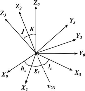
Figure 1: The four reference frames and the relevant angles related to the Andoyer (left) and Delaunay (right) canonical variables. See the text for more details.

2.2 Andoyer variables

For the rotational motion, following Deprit (1967), we adopt the Andoyer variables,

$$L_{s} =G_{s}\cos{J}\ , l_{s}\ ,$$

$$G_{s} \ , g_{s}\ ,$$

$$H_{s} =G_{s}\cos{K}\ , h_{s}\ ,$$

where $G_{s}$ is the norm of the angular momentum.

The Andoyer variables present two virtual singularities: for $J=0$, i.e., when the angular momentum is collinear with the direction of the axis of greatest inertia, and $K=0$, i.e., when the spin axis of rotation is perpendicular to the orbital plane. Therefore, we introduce the modified Andoyer variables, see Henrard (2005a),

$$L_{1} =\frac{G_{s}}{n_{o}C}\ , l_{1} =l_{s}+g_{s}+h_{s}\ ,$$ (1)

$$L_{2} =\frac{G_{s}-L_{s}}{n_{o}C}\ , l_{2} =-l_{s}\ ,$$

$$L_{3} =\frac{G_{s}-H_{s}}{n_{o}C}\ , l_{3} =-h_{s}\ ,$$

where $n_{o}$ is the orbital mean motion of the rotating body. Let us remark that this change of coordinates is a canonical transformation with multiplier $(n_{0}C)^{-1}$.

2.3 Delaunay variables

For the orbital motion, we introduce the classical Delaunay variables,

$$L_{o} =m\sqrt{\mu a}\ , l_{o} \ ,$$

$$G_{o} =L_{o}\sqrt{1-e^{2}}\ , g_{o} =\omega\ ,$$

$$H_{o} =G_{o}\cos{i}\ , h_{o} =\Omega\ ,$$

where $\mu=\mathcal{G}(m+M)$, $\mathcal{G}$ is the universal constant of gravitation, $a$ is the semi-major axis, $e$ the eccentricity and $i$ the inclination of the orbit described by the rotating body.

The Delaunay variables are singular for $e=0$ and $i=0$. Therefore, we introduce the modified Delaunay variables,

$$L_{4} =L_{o}\ , l_{4} =l_{o}+g_{o}+h_{o}\ ,$$ (2)

$$L_{5} =L_{o}-G_{o}\ , l_{5} =-g_{o}-h_{o}\ ,$$

$$L_{6} =G_{o}-H_{o}\ , l_{6} =-h_{o}\ .$$

Let us remark that $L_{5}$ and $L_{6}$ are of the same order of magnitude as the eccentricity, $e$, and inclination, $i$, respectively.

2.4 Free rotation

The rotational kinetic energy, Deprit (1967), reads

$$T=\frac{L_{s}^{2}}{2C}+\frac{1}{2}(G_{s}^{2}-L_{s}^{2})\left(\frac{\sin^{2}{l_{s}}}{A}+\frac{\cos^{2}{l_{s}}}{B}\right)\ .$$

Thus, in our set of variables, we get

$$\frac{T}{n_{o}C}=\frac{n_{o}L_{1}^{2}}{2}+\frac{n_{0}L_{3}(2L_{1}-L_{3})}{2}\left(\frac{\gamma_{1}+\gamma_{2}}{1-\gamma_{1}-\gamma_{2}}\sin^{2}(l_{3})+\frac{\gamma_{1}-\gamma_{2}}{1-\gamma_{1}+\gamma_{2}}\cos^{2}(l_{3})\right)\ ,$$

where

$$\gamma_{1}=\frac{2C-B-A}{2C}\quad\hbox{and}\quad\gamma_{2}=\frac{B-A}{2C}\ .$$

2.5 Perturbation by another body

The perturbation induced by the point body mass on the rotation of the rigid body, can be expressed via a gravitational potential, $V$, see, e.g., Henrard & Schwanen (2004) for a detailed exposition. The gravitational potential has the form

$$V=-{\mathcal{G}M}\iiint_{W}\frac{\varrho}{r}\,{\rm d}W\ ,$$

where $\varrho$ is the density inside the volume $W$ of the body and $r$ the distance between the point mass and a volume element inside the body. Using the classical expansion of the potential in spherical harmonics (see, e.g., Bertotti & Farinella(1990)), we get

$$V=-\frac{\mathcal{G}M}{r}\left(1+\sum_{n\geq 1}r^{-n}\sum_{m=0}^{n}P_{n}^{m}(\sin\varphi)\biggl{(}C_{n}^{m}\cos m\psi+S_{n}^{m}\sin m\psi\biggr{)}\right)\ ,$$

where $\varphi$ is the latitude and $\psi$ the longitude of the perturbing mass in the body frame. Limiting the expansion to the terms of order two and neglecting the first term $-{\mathcal{G}M}/r$, which does not affect the rotation, we have

$$V=\frac{3}{2}\frac{\mathcal{G}M}{a^{3}}\biggl{(}\frac{a}{r}\biggr{)}^{3}\left(C_{2}^{0}\bigl{(}x_{3}^{2}+y_{3}^{2}\bigr{)}-2C_{2}^{2}\bigl{(}x_{3}^{2}-y_{3}^{2}\bigr{)}\right)\ ,$$

where $(x_{3},y_{3},z_{3})$ are the components (in the body frame) of the unit vector pointing to the perturbing body. The coefficients $C_{2}^{0}$ and $C_{2}^{2}$, can be written in terms of the moments of inertia and of the dimensionless parameters $J_{2}$ and $C_{22}$, as

$$C_{2}^{0} =\frac{A+B-2C}{2}=-mR_{{\rm e}}^{2}J_{2}\ ,$$

$$C_{2}^{2} =\frac{B-A}{4}=mR_{{\rm e}}^{2}C_{22}\ .$$

Introducing the quantity $n_{o}^{*}=\sqrt{\mathcal{G}M/a^{3}}$, we get

$$\frac{V}{n_{o}C}=n_{0}\biggl{(}\frac{a}{r}\biggr{)}^{3}\left(\delta_{1}\bigl{(}x_{3}^{2}+y_{3}^{2}\bigr{)}+\delta_{2}\bigl{(}x_{3}^{2}-y_{3}^{2}\bigr{)}\right)\ ,$$ (3)

with

$$\delta_{1}=-\frac{3}{2}\left(\frac{n_{o}^{*}}{n_{o}}\right)^{2}\gamma_{1}\quad\hbox{and}\quad\delta_{2}=-\frac{3}{2}\left(\frac{n_{o}^{*}}{n_{o}}\right)^{2}\gamma_{2}\ .$$

In order to express the potential $V$ in terms of the canonical Andoyer-Delaunay variables, we use the following relation,

$$\left(\begin{array}[]{c}x_{3}\\ y_{3}\\ z_{3}\end{array}\right)=R_{3}(l_{s})R_{1}(J)R_{3}(g_{s})R_{1}(K)R_{3}(h_{s})R_{3}(-h_{o})R_{1}(-i_{o})R_{3}(-g_{o})\left(\begin{array}[]{c}\cos(v_{o})\\ \sin(v_{o})\\ 0\end{array}\right)\ ,$$

where $v_{o}$ is the true anomaly and $R_{i}$ are rotation matrices,

$$R_{1}(\varphi)=\begin{pmatrix}\phantom{-}\cos(\varphi)&\sin(\varphi)&0\\ -\sin(\varphi)&\cos(\varphi)&0\\ 0&0&1\end{pmatrix}\qquad\hbox{and}\qquad R_{3}(\varphi)=\begin{pmatrix}1&0&0\\ 0&\phantom{-}\cos(\varphi)&\sin(\varphi)\\ 0&-\sin(\varphi)&\cos(\varphi)\end{pmatrix}\ .$$

Finally, in order to get the expression of the potential in the canonical variables, we have to compute the expansions of $(a/r)^{3}$, $\cos(v_{o})$ and $\sin(v_{o})$ in terms of the eccentricity, $e$, and mean anomaly, $l_{o}$, see, e.g. Poincaré (1892, 1905).

2.6 The spin-orbit model

We now consider a simplified spin-orbit model, making some strong assumptions on the system. Similar assumptions have already been used in previous studies, see, e.g., Henrard & Schwanen (2004), Henrard (2005a, 2005b), Noyelles et al. (2008) and Lhotka (2013).

1. We assume that the wobble, $J$, is equal to zero. This means that the spin axis is aligned with respect to the direction of the axis of greatest inertia. Thus, we have

   $$\frac{T}{n_{o}C}=\frac{n_{o}L_{1}^{2}}{2}\ .$$

2. The rotating body is assumed to be locked in a $1$:$1$ spin-orbit resonance. We introduce the resonant variables

   $$\Sigma_{1} =L_{1}\ , \sigma_{1} =l_{1}-l_{4}\ ,$$ (4)

   $$\Sigma_{3} =L_{3}\ , \sigma_{3} =l_{3}-l_{6}\ ,$$

   and, after introducing these new coordinates, neglect the effects of the fast dynamics on the long-term evolution via an average over the angle, $l_{4}$, namely

   $$\langle V\rangle_{l_{4}}=\frac{1}{2\pi}\int_{0}^{2\pi}V\,{\rm d}l_{4}\ .$$

3. We neglect the influence of the rotation on the orbit of the body. Indeed, we assume that the orbital variables, see Eq. (2), are known functions of time acting as external parameters. Namely, we consider that the perturbing body lies on a slowly precessing eccentric orbit, with constant precession frequency $\dot{\Omega}\,$. The time dependence of the Hamiltonian can be modelled via the two angular variables,

   $$l_{4}(t)=n\,t+l_{4}(0)\qquad\hbox{and}\qquad l_{6}(t)=\dot{\Omega}\,t+l_{6}(0)\ .$$

Finally, we end up with a Hamiltonian that reads

$$H=\frac{n_{o}\Sigma_{1}^{2}}{2}-n_{o}\Sigma_{1}+\dot{\Omega}\Sigma_{3}+\langle V\rangle_{l_{4}}\ .$$ (5)

Taking into account a more general perturbed orbit (e.g., including the wobble and thus removing hypothesis (i) by adding one degree of freedom or replacing the first order average in (ii) by an higher order average), would not be difficult, but would introduce many supplementary parameters. The expanded Hamiltonian would have a form similar to Eq. (5), but, having more terms, it would be heavier from the computational point of view. In this work we want to focus on the estimate of the long-time stability around the Cassini state, thus we take this simplified spin-orbit model that keeps the relevant features of the system.

The Hamiltonian (5) possesses an equilibrium, the Cassini state, defined by

$$\sigma_{1} =0\ , \frac{\partial H}{\partial\Sigma_{1}} =0\ ,$$ (6)

$$\sigma_{3} =0\ , \frac{\partial H}{\partial\Sigma_{3}} =0\ .$$

We denote by $\Sigma_{1}^{*}$ and $\Sigma_{3}^{*}$ the values at the equilibrium. Geometrically, $\sigma_{1}=0$ means that the smallest axis of inertia points towards the perturbing body, while $\sigma_{3}=0$ means that the nodes of the orbit and equator are locked. The values $\Sigma_{1}^{*}$ and $\Sigma_{3}^{*}$, correspond to fixing the inertial obliquity $K^{*}$. Finally, $\Sigma_{1}^{*}-1$ is a small correction of the unperturbed spin frequency, $n_{0}\Sigma_{1}^{*}$.

3 Stability around the Cassini state

We now aim to study the dynamics in the neighborhood of the Cassini state defined here above. We introduce the translated canonical variables

$$\Delta\Sigma_{1}=\Sigma_{1}-\Sigma_{1}^{*}\ ,\qquad\sigma_{1}\ ,$$ (7)

$$\Delta\Sigma_{3}=\Sigma_{3}-\Sigma_{3}^{*}\ ,\qquad\sigma_{3}\ ,$$

and, with a little abuse of notation, in the following we will denote again $\Delta\Sigma_{i}$ by $\Sigma_{i}$, with $i=1,\,3\,$. Let us also introduce the shorthand notations $\Sigma=(\Sigma_{1},\Sigma_{3})$ and $\sigma=(\sigma_{1},\sigma_{3})\,$. In these new coordinates, the equilibrium is set at the origin, thus we can expand the Hamiltonian (5) in power series of $(\Sigma,\,\sigma)$. Let us remark that the linear terms disappear, as the origin is an equilibrium, thus the lowest order terms in the expansion are quadratic in $(\Sigma,\,\sigma)\,$. Precisely, we can write the Hamiltonian as

$$H(\Sigma,\sigma)=H_{0}(\Sigma,\sigma)+\sum_{j>0}H_{j}(\Sigma,\sigma)\ ,$$ (8)

where $H_{j}$ is an homogeneous polynomial of degree $j+2$ in $(\Sigma,\,\sigma)\,$. In the latter equation the quadratic term, $H_{0}$, has been separated in view of its relevance in the perturbative scheme. The analytical expression of $H_{0}$ can be found in the Appendix A of Henrard & Schwanen (2004).

3.1 Diagonalization of the quadratic part

The quadratic part of the Hamiltonian reads

$$H_{0}(\Sigma,\sigma)= \mu_{{\scriptscriptstyle\Sigma_{1}\Sigma_{1}}}\Sigma_{1}^{2}+2\mu_{{\scriptscriptstyle\Sigma_{1}\Sigma_{3}}}\Sigma_{1}\Sigma_{3}+\mu_{{\scriptscriptstyle\Sigma_{3}\Sigma_{3}}}\Sigma_{3}^{2}$$

$$+\mu_{{\scriptscriptstyle\sigma_{1}\sigma_{1}}}\sigma_{1}^{2}+2\mu_{{\scriptscriptstyle\sigma_{1}\sigma_{3}}}\sigma_{1}\sigma_{3}+\mu_{{\scriptscriptstyle\sigma_{3}\sigma_{3}}}\sigma_{3}^{2}\ .$$

Following the approach of Henrard & Schwanen (2004), we introduce a canonical transformation to reduce the Hamiltonian $H_{0}$ to a sum of squares,

$$\Sigma_{1} =(1-\alpha\beta)\Sigma_{1}^{\prime}-\alpha\Sigma_{3}^{\prime}\ , \sigma_{1} =\sigma_{1}^{\prime}-\beta\sigma_{3}^{\prime}\ ,$$ (9)

$$\Sigma_{3} =\beta\Sigma_{1}^{\prime}+\Sigma_{3}^{\prime}\ , \sigma_{3} =\alpha\sigma_{1}^{\prime}+(1-\alpha\beta)\sigma_{3}^{\prime}\ ,$$

where the parameter $\alpha$ and $\beta$ have to be chosen to get rid of the mixed terms in $H_{0}$, namely,

$$\beta\mu_{{\scriptscriptstyle\sigma_{1}\sigma_{1}}}-(1-2\alpha\beta)\mu_{{\scriptscriptstyle\sigma_{1}\sigma_{3}}}-\alpha(1-\alpha\beta)\mu_{{\scriptscriptstyle\sigma_{3}\sigma_{3}}}=0\ ,$$

$$\alpha(1-\alpha\beta)\mu_{{\scriptscriptstyle\Sigma_{1}\Sigma_{1}}}-(1-2\alpha\beta)\mu_{{\scriptscriptstyle\Sigma_{1}\Sigma_{3}}}-\beta\mu_{{\scriptscriptstyle\Sigma_{3}\sigma_{3}}}=0\ .$$

This change of coordinates is the so-called “untangling transformation”, see Henrard & Lemaître (2005), and permits to write $H_{0}$ as

$$H_{0}(\Sigma^{\prime},\sigma^{\prime})=\left(\mu^{\prime}_{{\scriptscriptstyle\Sigma_{1}^{\prime}\Sigma_{1}^{\prime}}}\Sigma_{1}^{\prime 2}+\mu^{\prime}_{{\scriptscriptstyle\sigma_{1}^{\prime}\sigma_{1}^{\prime}}}\sigma_{1}^{\prime 2}\right)+\left(\mu^{\prime}_{{\scriptscriptstyle\Sigma_{3}^{\prime}\Sigma_{3}^{\prime}}}\Sigma_{3}^{\prime 2}+\mu^{\prime}_{{\scriptscriptstyle\sigma_{3}^{\prime}\sigma_{3}^{\prime}}}\sigma_{3}^{\prime 2}\right)\ .$$ (10)

Thus, if the products of the coefficients $\mu^{\prime}_{{\scriptscriptstyle\Sigma_{i}^{\prime}\Sigma_{i}^{\prime}}}$ and $\mu^{\prime}_{{\scriptscriptstyle\sigma_{i}^{\prime}\sigma_{i}^{\prime}}}$, with $i=1,\,3\,$, are positive the quadratic part of the Hamiltonian describes a couple of harmonic oscillators.

We now perform a rescaling and introduce the polar coordinates,

$$\Sigma_{1}^{\prime} =\sqrt{2U_{1}/U_{1}^{*}}\cos(u_{1})\ ,\qquad\sigma_{1}^{\prime}=\sqrt{2U_{1}U_{1}^{*}}\sin(u_{1})\ ,$$ (11)

$$\Sigma_{3}^{\prime} =\sqrt{2U_{3}/U_{3}^{*}}\cos(u_{3})\ ,\qquad\sigma_{3}^{\prime}=\sqrt{2U_{3}U_{3}^{*}}\sin(u_{3})\ ,$$

where

$$U_{1}^{*}=\sqrt{\mu^{\prime}_{{\scriptscriptstyle\Sigma_{1}^{\prime}\Sigma_{1}^{\prime}}}/\mu^{\prime}_{{\scriptscriptstyle\sigma_{1}^{\prime}\sigma_{1}^{\prime}}}}\ ,\qquad\hbox{and}\qquad U_{3}^{*}=\sqrt{\mu^{\prime}_{{\scriptscriptstyle\Sigma_{3}^{\prime}\Sigma_{3}^{\prime}}}/\mu^{\prime}_{{\scriptscriptstyle\sigma_{3}^{\prime}\sigma_{3}^{\prime}}}}\ .$$

After this last transformation, the quadratic part of the Hamiltonian is expressed in action-angle variables and reads

$$H_{0}=\omega_{u_{1}}U_{1}+\omega_{u_{3}}U_{3}\ ,$$

where $\omega_{u_{1}}$ and $\omega_{u_{3}}$ are the frequencies of the angular variables $u_{1}$ and $u_{3}$, respectively. Again, we introduce the shorthand notations $U=(U_{1},\,U_{3})\,$, $u=(u_{1},\,u_{3})$ and $\omega_{u}=(\omega_{u_{1}},\,\omega_{u_{3}})\,$.

Finally, we apply the same transformations that allow to introduce the action-angle variables for the quadratic term, i.e., equations (10) and (11), to the full Hamiltonian (8). In these new coordinates, the transformed Hamiltonian can be expanded in Taylor-Fourier series and reads

$$H^{(0)}(U,\,u)=\omega_{u}\cdot U+\sum_{j>0}H^{(0)}_{j}(U,\,u)\ ,$$ (12)

where the terms $H_{j}$ are homogeneous polynomials of degree $j/2+1$ in $U$, whose coefficients are trigonometric polynomials in the angles $u\,$.

The Hamiltonian (12) has the form of a perturbed system of harmonic oscillators, thus we are led to study the stability of the equilibrium, placed at the origin, corresponding to the Cassini state. Let us stress that the change of coordinates in Eq. (11) is singular at the origin, nevertheless, this virtual singularity is harmless as we will just be interested in giving a bound of an analytic function in a disc around the origin. Moreover, one could adopt the cartesian coordinates avoiding the singularity problem. We now aim to investigate the stability of the equilibrium in the light of Nekhoroshev theory, introducing the so-called effective stability time.

3.2 Birkhoff normal form

Following a quite standard procedure we construct the Birkhoff normal form for the Hamiltonian (12) (see Birkhoff (1927); for an application of Nekhoroshev theory see, e.g., Giorgilli (1988)). This is a well known topic, thus we limit our exposition to a short sketch adapted to the present context.

The aim is to give the Hamiltonian the normal form at order $r$

$$H^{(r)}(U,\,u)=Z_{0}(U)+\ldots+Z_{r}(U)+\sum_{s>r}\mathcal{R}^{(r)}_{s}(U,\,u)\ ,$$ (13)

where $Z_{s}$, for $s=0,\,\ldots\,,r\,$, is a homogeneous polynomial of degree $s/2+1$ in $U$ and in particular it is zero for odd $s$. The unnormalized reminder terms $\mathcal{R}^{(r)}_{s}$, for $s>r$, are homogeneous polynomials of degree $s/2+1$ in $U$, whose coefficients are trigonometric polynomials in the angles $u\,$.

We proceed by induction. For $r=0$ the Hamiltonian (12) is already in Birkhoff normal form. Assume that the Hamiltonian is in normal form up to a given order $r>0$, we determine the generating function $\chi^{(r+1)}$ and the normal form term $Z_{r+1}$, by solving the equation

$$\left\{\chi^{(r+1)},\,\omega_{u}\cdot U\right\}+\mathcal{R}^{(r)}_{r+1}(U,\,u)=Z_{r+1}(U)\ ,$$

where $\{\cdot,\cdot\}$ denotes the usual Poisson bracket. Using the Lie series algorithm, see, e.g., Henrard (1973) and Giorgilli (1995), we compute the new Hamiltonian as $H^{(r+1)}=\exp(L_{\chi^{(r+1)}})H^{(r)}\,$. It is easy to show that $H^{(r+1)}$ has a form analogous to Eq. (13) with new functions $\mathcal{R}^{(r+1)}_{s}$ of degree $s/2+1$ (with $s>r+1$) and the normal form part ending with $Z_{r+1}$ , which is equal to zero if $r$ is even. As usual when using Lie series methods, with a little abuse of notation, we denote again by $(U,\,u)$ the new coordinates.

This algorithm can be iterated up to the order $r$ provided that the non-resonance condition

$$k\cdot\omega_{u}\neq 0\qquad\hbox{for }k=(k_{1},\,k_{2})\in\mathbb{Z}^{2}\hbox{ such that }0<|k|_{1}\leq r+2\ ,$$

is fulfilled, where we used the usual notation $|k|_{1}=|k_{1}|+|k_{2}|$.

3.3 Effective stability

It is well known that the Birkhoff normal form at any finite order $r$ is convergent in some neighborhood of the origin, but the analyticity radius shrinks to zero when the order $r\to\infty\,$. Thus, the best strategy is to look for stability over a finite time, possibly long enough with respect to the lifetime of the system. We concentrate here on the quantitative estimates that allow to give an upper bound of the effective stability time that has to be evaluated.

Let us pick two positive numbers $R_{1}$ and $R_{3}$, and consider a polydisk $\Delta_{\varrho R}$ centered at the origin of $\mathbb{R}^{2}$, defined as

$$\Delta_{\varrho R}=\left\{U\in\mathbb{R}^{2}:|U_{j}|\leq\varrho R_{j}\ ,\ j=1,3\right\}\ ,$$

$\varrho>0$ being a parameter.

Let us consider a function

$$f_{s}(U,\,u)=\sum_{|l|=s+2,k\in\mathbb{Z}^{2}}f_{l,k}\,U^{l/2}{\sin\atop\cos}(k\cdot u)\ ,$$

which is a homogeneous polynomial of degree $s/2+1$ in the actions $U$ and depends on the angles $u$. We define the quantity $|f_{s}|_{R}$ as

$$|f_{s}|_{R}=\sum_{|l|=s+2,k\in\mathbb{Z}^{2}}|f_{l,k}|R_{1}^{l_{1}/2}R_{3}^{l_{2}/2}\ .$$

Thus we get the estimate

$$|f(U,u)|\leq|f|_{R}\,\varrho^{s/2+1}\ ,\quad\hbox{for }U\in\Delta_{\varrho R}\,,\ u\in\mathbb{T}^{2}\ .$$

Let now $U(0)\in\Delta_{\varrho_{0}R}$, with $\varrho_{0}<\varrho$. Then we have $U(t)\in\Delta_{\varrho R}$ for $t\leq T$, where $T$ is the escape time from the domain $\Delta_{\varrho R}$. This is the effective stability time that we want to evaluate. We consider the trivial estimate

$$|U(t)-U(0)|\leq|t|\cdot\sup|\dot{U}|\ ,$$

thus we need to bound the quantity $\sup|\dot{U}|$. To this end, taking the Hamiltonian (13), which is in Birkhoff normal form up to order $r$, we get

$$|\dot{U}|\leq|\{U,H^{(r)}\}|=\sum_{s>r}|\{U,\mathcal{R}^{(r)}_{s}\}|\leq c|\{U,\mathcal{R}^{(r)}_{r+1}\}|_{R}\,\varrho^{r/2+1}\ ,$$

with $c\geq 1$. In fact, after having set $\varrho$ smaller than the convergence radius of the remainder series, $\mathcal{R}^{(r)}_{s}$ for $s>r$, the above inequality holds true for some value $c$.

The latter equation allows us to find a lower bound for the escape time from the domain $\Delta_{\varrho R}$, namely

$$\tau(\varrho_{0},\varrho,r)=\frac{\varrho-\varrho_{0}}{c|\{U,\mathcal{R}^{(r)}_{r+1}\}|_{R}\,\varrho^{r/2+1}}\ ,$$ (14)

which, however, depends on $\varrho_{0}$, $\varrho$, and $r$. Let us emphasize that $\varrho_{0}$ is the only physical parameter, being fixed by the initial data, while $\varrho$, and $r$ are left arbitrary. Indeed, the parameter $\varrho_{0}$ must be chosen in such a way that the domain $\Delta_{\varrho_{0}R}$ contains the initial conditions of the system. Thus we try to find an estimate of the escape time, $T(\varrho_{0})$, depending only on the physical parameter $\varrho_{0}$.

We optimize $\tau(\varrho_{0},\varrho,r)$ with respect to $\varrho$ and $r$, proceeding as follows. First we keep $r$ fixed, and remark that the function $\tau(\varrho_{0},\varrho,r)$ has a maximum for

$$\varrho_{\rm opt}=\frac{r+2}{r}\varrho_{0}\ .$$

This gives an optimal value of $\varrho$ as a function of $\varrho_{0}$ and $r$, thus we define

$$\widetilde{\tau}(\varrho_{0},r)=\tau(\varrho_{0},\varrho_{\rm opt},r)\ .$$

Finally, we look for the optimal value $r_{\rm opt}$ of the normalization order, which maximizes $\widetilde{\tau}(\varrho_{0},r)$. Namely, we look for the quantity

$$T(\varrho_{0})=\max_{r\geq 1}\widetilde{\tau}(\varrho_{0},r)\ ,$$

which is our best estimate of the escape time, we define this quantity as the effective stability time.

4 Application to Titan

We now come to the application of our study to the largest moon of Saturn, Titan. Let us stress that we take a simplified model: we consider Titan as a rigid body orbiting around Saturn, regarded as a point body mass. Moreover, we keep all the assumptions that we have made in Subsection 2.6 for the spin-orbit model. Concerning the hypothesis (iii), i.e., the constant precession frequency $\dot{\Omega}\,$, we remark that in this case is not restrictive. Indeed, for Titan, the expansion of $\dot{\Omega}$ has a dominant term, while the other ones are negligible, see Vienne & Duriez (1995) (Table 6d).

We first make an expansion of the Hamiltonian (5) up to degree $8$ in the eccentricity, by using the Wolfram Mathematica software. Then, we express the Hamiltonian in the canonical Andoyer-Delaunay variables, see equations (1) and (2), and introduce the resonant coordinates $(\Sigma,\,\sigma)$, defined in Eq. (4). In the actual computation we take the physical parameters reported in Table 1.

Table 1: Titan physical parameters. The parameters related to the gravity field and shape of Titan, $J_{2}$, $C_{22}$ and $C/MR_{\rm e}^{2}$, are taken from Iess et al. (2010). The orbital data are taken from Vienne & Duriez (1995).

$|^{|^{|}}$ $M$	$\phantom{-}5.683200\times 10^{+26}\,$ Kg
$J_{2}$	$\phantom{-}3.180800\times 10^{-5}$
$C_{22}$	$\phantom{-}9.983000\times 10^{-6}$
$C/MR_{\rm e}^{2}$	$\phantom{-}3.414000\times 10^{-1}$
$a$	$\phantom{-}1.221865\times 10^{+6}\,$ Km
$e$	$\phantom{-}2.890000\times 10^{-2}$
$i$	$\phantom{-}5.579818\times 10^{-3}\,$ rad
$\dot{\Omega}$	$-8.931240\times 10^{-3}\,$ rad/year
$n_{o}$	$\phantom{-}1.439240\times 10^{+2}\,$ rad/year

A numerical solution of Eq. (6) gives $\Sigma_{1}^{*}=1+1.829\times 10^{-9}$ and $\Sigma_{3}^{*}=2.947\times 10^{-5}$. These are the values at the equilibrium, the Cassini state; thus we expand the Hamiltonian (8) in the translated canonical variables, see Eq. (7). Following the procedure in Subsection 3.1, we perform the so-called “untangling transformation”, see Eq. (9) and introduce the action-angle variables $(U,\,u)\,$, where $U_{1}^{*}=5.348\times 10^{1}$ and $U_{3}^{*}=1.696\times 10^{4}$. This allows us to write the Hamiltonian as

$$H^{(0)}(U,\,u)=\omega_{u}\cdot U+\sum_{j>0}H^{(0)}_{j}(U,\,u)\ ,$$

with $\omega_{u_{1}}=2.690$ and $\omega_{u_{3}}=2.375\times 10^{-2}\,$. More details concerning the semi-analytical expansion of the Hamiltonian, including the explicit form of some relevant quantities, are reported in Appendix A. We now compute a high-order Birkhoff normal form up to order $r=30$, see Eq. (13), by using a specially devised algebraic manipulator, see Giorgilli & Sansottera (2011). As shown in Subsection 3.3, the estimate of the effective stability time is now straightforward. Let us remark that, in this specific case, it is enough to set $c=2$ in Eq. (14).

First, we give an estimate of the stability time as a function of the parameter $\varrho_{0}$, that parametrizes the radius of the polydisk containing the initial data. Let us remark that $\varrho_{0}=0$ corresponds to the exact Cassini state, while taking $\varrho_{0}>0$ allows small oscillations around the equilibrium point. The results of our computations are reported in Figure 2. The best estimate corresponds to the highest order of normalization, namely $r=30$, however already at order $r=20$ we obtain really good estimates. As shown in the plot, we reach an effective stability time greatly exceeding the estimated age of the Universe in a domain $\Delta_{R}$ that roughly corresponds to a libration of $0.1$ radians. Quoting J.E. Littlewood in his papers about the stability of the Lagrangian equilateral equilibria of the problem of three bodies, “while not eternity, this is a considerable slice of it.”.

2(a):

2(b):

Figure 2: Evaluation of the estimated effective stability time. The time unit is the year. In 2 we report the effective stability time evaluated according to the algorithm described in Subsection 3.3. The three lines correspond (from down to top) to three different normalization orders: $r=10$ (blue), $r=20$ (pink) and $r=30$ (red). In 2–2 we report the effective stability time as a function of the mean inclination, $i$, (continued on the following page)

2(c):

2(d):

Figure 2: (continued from the previous page) the mean precession of the ascending node of Titan orbit, $\dot{\Omega}\,$ and the normalized greatest moment of inertia, $C/MR_{\rm e}^{2}$. The colors refer to the stability time (in logarithmic scale), the yellow region is the most stable one.

Finally, we investigate the dependence of the effective stability time on three relevant physical parameters: the orbital inclination, $i$, the mean precession of the ascending node of Titan orbit, $\dot{\Omega}$, and the polar moment of inertia, $C$.

The results for the investigation of the stability time as a function of $i$ and $\dot{\Omega}\,$, is reported in Figure 2. The effective stability time turns out to grow up for increasing values of the inclination, while the dependence on the precession of the ascending node is less significant. In Figure 2 we report the outcome of our computations of the effective stability time as a function of $C/MR_{\rm e}^{2}$ and $\dot{\Omega}\,$. We let vary the parameter $C/MR_{\rm e}^{2}$ in the range $[0.3,0.4]$. This interval should guarantee that we include the true value of the parameter, as for the Galilean satellites of Jupiter. We see that the effective stability time decreases for both increasing values of the normalized greatest moment of inertia and precession of the ascending node. The dependence of the stability time on the parameters $i$ and $C/MR_{\rm e}^{2}$ is reported in Figure 2. Again the effective stability time is growing for increasing values of the inclination, while the parameter $C/MR_{\rm e}^{2}$, in this case, is less important.

5 Conclusions and outlook

We have studied the long-time stability around the Cassini state in the spin-orbit problem. As explained in details in Section 2 and 3, the Hamiltonian of the system turns out to have the form of a perturbed system of harmonic oscillators. We have computed a high-order Birkhoff normal form that allows us to obtain an analytical estimate of the effective stability time around the Cassini state.

Our aim was to investigate the physical relevance of the long-time stability in the framework of the Nekhoroshev theory. For this reason we used a simplified spin-orbit model that keeps all the relevant features of the system. Taking a more general model into account, would not substantially change the form of the Hamiltonian and certainly deserves to be studied in the future.

The main conclusion is that our estimates are physically relevant. We investigate a region of the parameters that contains the real data of Titan and the stability around the Cassini state is assured over very long times, largely exceeding the age of the Universe. Therefore, our work is a further confirmation that the long-time stability predicted by Nekhoroshev theory may be very relevant for physical systems.

The effective stability time depends on many physical parameters, e.g., the mean inclination, $i$, the mean precession rate, $\dot{\Omega}$ and the greatest moment of inertia, $C$. These parameters play a crucial role in understanding Titan rotation and their estimation is a major challenge. As shown in the last part of the previous section, our method can be used to determine the most stable region of the parameters and supports the estimates given by observations.

The natural question is how far these results can be extended considering more realistic models. On the one hand, let us recall that the simplified spin-orbit model we adopt, makes strong assumptions on the system. Thus, our model might be less perturbed than the real system, and therefore more stable. However, if the question concerns the stability around the Cassini state, meaning that we just look for bounds on the librations, then further terms in the Hamiltonian would be relevant only if they produce resonances that make their size in the perturbation expansions to grow, due to the small divisors. Indeed, all our estimates of the stability time are based on the evaluation of the size of the perturbing terms. Finally, let us remark that our method is strongly based on Hamiltonian theory, thus other non conservative effects cannot be taken into account in this framework.

Appendix A Semi-analytical expansion of the Hamiltonian (Titan application)

We report here the explicit expansions of the relevant Hamiltonian functions related to the application to Titan. We recall that the Titan physical parameters adopted here are reported in Table 1.

The averaged potential in Eq. (5) takes the form

$$\langle V\rangle_{l_{4}}= -1.01\times 10^{-2}\cos^{2}K-3.13\times 10^{-7}\sin^{2}K$$

$$-1.12\times 10^{-4}\cos\left(\sigma_{3}\right)\cos K\sin K$$

$$-\cos\left(2\sigma_{1}\right)\left(3.14\times 10^{-3}+6.29\times 10^{-3}\cos K+3.14\times 10^{-3}\cos^{2}K\right)$$

$$+\cos\left(2\sigma_{3}\right)\left(1.56\times 10^{-7}\cos^{2}K-1.56\times 10^{-7}\right)$$

$$-\cos\left(2\sigma_{1}+\sigma_{3}\right)\left(3.51\times 10^{-5}\cos K+3.51\times 10^{-5}\right)\sin K$$

$$+\cos\left(2\sigma_{1}+2\sigma_{3}\right)\left(4.90\times 10^{-8}\cos^{2}K-9.79\times 10^{-8}\sin^{2}K-4.90\times 10^{-8}\right)$$

$$+\cos\left(2\sigma_{1}+3\sigma_{3}\right)\left(2.73\times 10^{-10}\cos K-2.73\times 10^{-10}\right)\sin K$$

$$-1.91\times 10^{-13}\cos\left(2\sigma_{1}+4\sigma_{3}\right)\left(1.00-1.00\cos K\right)^{2}\ .$$

The quadratic part of the Hamiltonian (8), $H_{0}$, reads

$$H_{0} =2.52\times 10^{-2}\sigma_{1}^{2}+1.08\times 10^{-6}\sigma_{1}\sigma_{3}+7.00\times 10^{-7}\sigma_{3}^{2}$$

$$\quad+7.20\times 10^{1}\Sigma_{1}^{2}-2.08\times 10^{-2}\Sigma_{1}\Sigma_{3}+2.01\times 10^{2}\Sigma_{3}^{2}\ ,$$

and the values of the parameter $\alpha$ and $\beta$ corresponding to the untangling transformation, see Eq. (9), are $\alpha=-8.46\times 10^{-5}$ and $\beta=2.14\times 10^{-5}\,$. Thus, the quadratic part of the Hamiltonian (10) in diagonal form reads

$$H_{0}=2.52\times 10^{-2}\sigma_{1}^{2}+7.00\times 10^{-7}\sigma_{3}^{2}+7.20\times 10^{1}\Sigma_{1}^{2}+2.01\times 10^{2}\Sigma_{3}^{2}\ .$$

The parameters $U_{1}^{*}$ and $U_{3}^{*}$ related to the rescaled polar coordinates, see Eq. (11), take the values $U_{1*}=5.348\times 10^{1}$ and $U_{3*}=1.696\times 10^{4}\,$, and the quadratic part of the Hamiltonian in action angle variables, see Eq. (12), reads

$$H_{0}=2.69\,U_{1}+2.37\times 10^{-2}U_{3}\ ,$$

while the term of order $3$ in Eq. (12), $H^{(0)}_{1}\,$, reads

$$H^{(0)}_{1}= 2.86\times 10^{-7}\cos(u_{1})\sqrt{U_{1}}^{3}-2.87\times 10^{-7}\cos(3u_{1})\sqrt{U_{1}}^{3}$$

$$+1.98\times 10^{-3}\cos(2u_{1}-u_{3})U_{1}\sqrt{U_{3}}-3.99\times 10^{-3}\cos(u_{3})U_{1}\sqrt{U_{3}}$$

$$+2.01\times 10^{-3}\cos(2u_{1}+u_{3})U_{1}\sqrt{U_{3}}-3.97\times 10^{-3}\cos(u_{1})\sqrt{U_{1}}U_{3}$$

$$+9.29\times 10^{-2}\cos(u_{1}-2u_{3})\sqrt{U_{1}}U_{3}-9.62\times 10^{-2}\cos(u_{1}+2u_{3})\sqrt{U_{1}}U_{3}$$

$$-2.19\cos(u_{3})\sqrt{U_{3}}^{3}-2.19\cos(3u_{3})\sqrt{U_{3}}^{3}\ .$$

We provide the approximation of Eq. (12), up to order $6$ in $\left(\sqrt{U_{1}}\,,\ \sqrt{U_{3}}\,\right)\,$, in the electronic Supplemental Material (see Table 2) while we report below the number of coefficients in Eq. (12) at each order,

Order	2	3	4	5	6	7	8	9	10	11	12	13	14	15	16
#terms	2	10	19	28	44	54	70	84	93	105	112	125	130	143	145

.

Finally, we report in the electronic Supplemental Material (see Table 3) the truncated normal form, up to order $12$. In this case the number of terms of order $2r$ in $\left(\sqrt{U_{1}}\,,\ \sqrt{U_{3}}\,\right)$ is just equal to $r+1\,$, thus, at each order, we report in the table below the number of coefficients in the remainder term at different orders

Order	3	4	5	6	7	8	9	10	11	12	13	14	15	16
#terms	10	19	28	44	60	85	110	146	182	231	280	345	423	544

.

References

- Beletskii (1972) V.V. Beletskii: Resonance rotation of celestial bodies and Cassini’s laws, CeMDA, 6, 356–378 (1972).
- Bertotti & Farinella (1990) B. Bertotti and P. Farinella: Physics of the Earth and the Solar System, Springer, Geophysics and Astrophysics Monographs, 31, (1990).
- Birkhoff (1927) G.D. Birkhoff: Dynamical systems, AMS, Colloquium publications 9, (1927).
- Bouquillon et al. (2003) S. Bouquillon, H. Kinoshita and J. Souchay: Extension of Cassini’s Laws, CeMDA, 86, 29–57 (2003).
- Cassini (1693) G.D. Cassini: Traité de l’origine et des progrès de l’Astronomie, Paris (1693).
- Colombo (1966) G. Colombo: Cassini’s Second and Third Laws, AJ, 71, 891–896 (1966).
- Deprit (1967) A. Deprit: Free rotation of a rigid body studied in the phase plane, AJP, 35, 424–428 (1967).
- D’Hoedt & Lemaître (2004) S. D’Hoedt and A. Lemaître: The spin-orbit resonant rotation of Mercury: A two degree of freedom Hamiltonian model, CeMDA, 89, 267–283 (2004).
- Giorgilli (1988) A. Giorgilli: Rigorous results on the power expansions for the integrals of a Hamiltonian system near an elliptic equilibrium point, Annales de l’I. H. P., 48, 423–439 (1988).
- Giorgilli (1995) A. Giorgilli: Quantitative methods in classical perturbation theory, NATO Advanced Study Institute on From Newton to Chaos, 21–37 (1995).
- Giorgilli et al. (2009) A. Giorgilli, U. Locatelli and M. Sansottera: Kolmogorov and Nekhoroshev theory for the problem of three bodies, CeMDA, 104, 159–173 (2009).
- Giorgilli et al. (2010) A. Giorgilli, U. Locatelli and M. Sansottera: Su un’estensione della teoria di Lagrange per i moti secolari, Rend. Ist. Lom., 143, 223–239 (2010).
- Giorgilli & Sansottera (2011) A. Giorgilli and M. Sansottera: Methods of algebraic manipulation in perturbation theory, Workshop Series of the Asociación Argentina de Astronomía, 3, 147–183 (2011).
- Goldreich & Peale (1966) P. Goldreich and S. Peale: Spin-orbit coupling in the solar system, AJ, 71, 425–437 (1966).
- Henrard (1973) J. Henrard: The Algorithm of the Inverse for Lie Transform, Recent Advances in Dynamical Astronomy, Astrophysics and Space Science Library, 39, 250–259 (1973).
- Henrard & Murigande (1987) J. Henrard and C. Murigande: Colombo’s top, CeMDA, 40, 345–366 (1987).
- Henrard & Schwanen (2004) J. Henrard and G. Schwanen: Rotation of Synchronous Satellites, Application to the Galilean Satellites, CeMDA, 89, 181–199 (2004).
- Henrard (2005a) J. Henrard: The rotation of Io, Icarus, 178, 144–153 (2005a).
- Henrard (2005b) J. Henrard: The Rotation of Europa, CeMDA, 91, 131–149 (2005b).
- Henrard & Lemaître (2005) J. Henrard and A. Lemaître: The untangling transformation, AJ, 130, 2415–2417 (2005).
- Iess et al. (2010) L. Iess, J. Rappaport, A. Jacobson, P. Racioppa and D.J. Stevenson: Gravity Field Shape and Moment of Inertia of Titan, Science, 327, 1367–1369 (2010).
- Lemaître et al. (2006) A. Lemaître, S. D’Hoedt and N. Rambaux: The 3:2 spin-orbit resonant motion of Mercury, CeMDA, 95, 213–224 (2006).
- Lhotka (2013) C. Lhotka: A symplectic mapping for the synchronous spin-orbit problem, CeMDA, 115, 405–426 (2013).
- Nekhoroshev (1977) N.N. Nekhoroshev: Exponential estimates of the stability time of near-integrable Hamiltonian systems, Russ. Math. Surveys, 32, 1–65 (1977).
- Nekhoroshev (1979) N.N. Nekhoroshev: Exponential estimates of the stability time of near-integrable Hamiltonian systems, II. Trudy Sem. Petrovs., 5, 5–50 (1979).
- Noyelles et al. (2008) B. Noyelles, A. Lemaître and A. Vienne: Titan’s rotation. A 3-dimensional theory, A&A, 478, 959–970 (2008).
- Peale (1969) S.J. Peale: Generalized Cassini’s Laws, AJ, 74, 483–489 (1969).
- Poincaré (1892) H. Poincaré: Les méthodes nouvelles de la Mécanique Céleste, Gauthier-Villars, Paris (1892).
- Poincaré (1905) H. Poincaré: Leçons de Mécanique Céleste, tomes I-II, Gauthier-Villars, Paris (1905).
- Sansottera et al. (2011) M. Sansottera, U. Locatelli and A. Giorgilli: On the stability of the secular evolution of the planar Sun-Jupiter-Saturn-Uranus system, Math. and Comp. in Sim., 88, 1–14 (2013).
- Steichen & Giorgilli (1997) D. Steichen and A. Giorgilli: Long Time Stability for the Main Problem of Artificial Satellites, CeMDA, 69, 317–330 (1997).
- Vienne & Duriez (1995) A. Vienne and L. Duriez: TASS1.6: Ephemerides of the major Saturnian satellites, A&A, 297, 588–605 (1995).
- Ward (1975) W.R. Ward: Tidal friction and generalized Cassini’s laws in the solar system, AJ, 80, 64–70 (1975).