On higher order radiative corrections to elastic electron-proton scattering

Abstract

QED radiative corrections to elastic electron-proton scattering at low energies are discussed. Corrections to the electron line and effects due to vacuum polarization are computed. Higher order effects are estimated for the conditions of the experiment on the electric and magnetic proton form factors by A1 Collaboration. Calculations are performed within the next-to-leading approximation. Inclusion of the higher order effects can affect the value of the proton charge radius extracted from the experimental data.

1 Introduction

First of all, our paper is motivated by recent very accurate experimental measurements of the electron-proton elastic scattering at the Mainz Microtron (MAMI) Bernauer:2013tpr . The average point-to-point errors in the cross sections measurement was of the order of a few permille.

Besides extraction of the proton electromagnetic form factors, the experiment managed to define the value of the proton electric charge radius with high precision. It is worth to note that the result for the charge radius extracted from the electron-proton scattering data was found to be inconsistent with the one obtained from muonic hydrogen Antognini:1900ns . The disagreement stimulates theoretical studies aimed at its resolution. In the present paper we are going to discuss several effects which can affect the data analysis of low-energy elastic electron-proton scattering.

The high precision of the experimental measurement of the differential cross section provides the clear requirement on the magnitude of effects which should be taken into account. We assume that aiming at the one-permille accuracy, we have to treat systematically all relative corrections being at least of $10^{-4}$ size.

2 Preliminaries and Notation

Let us consider the process

$$e(p_{1})+p(P_{1})\longrightarrow e(p_{2})+p(P_{2})+(n\gamma,\ e^{+}e^{-}).$$ (1)

The initial electron energy $E_{1}=p_{1}^{0}\equiv E$ is of the order 1 GeV, $E\gg m_{e}$. The momentum transfer squared $Q^{2}=-(p_{2}-p_{1})^{2}$ will be taken in the range $0.003<Q^{2}<1$ GeV² which was explored in the experiment. Note that the condition $Q^{2}\gg m_{e}^{2}$ holds for the whole range. The differential cross section ${d\sigma}/{d\Omega_{e}}$ of process (1) will be considered.

One-loop QED corrections to the process under consideration are well known. They are naturally separated into the following parts:
— real and virtual corrections to the electron line,
— real and virtual corrections to the proton line,
— interference of amplitudes of the first two types,
— the effect due to vacuum polarization. The corresponding analytic results were reproduced in Bernauer:2013tpr Among one-loop corrections, there is still an open discussion about the proper treatment of double photon exchange contributions, see e.g. papers Arrington:2011dn ; Lee:2015jqa and references therein. We agree with the importance of this point, but it goes beyond the scope of our present study.

To estimate the numerical effect of radiative corrections one has to take into account concrete experimental conditions. Of course, to get the final answer one should include the corrections into the whole program of the data analysis. But our task here will be just to present analytic results with simple estimates of their impact. So we will simplify the set-up (still following the main features of the experiment):
— we assume that the measurement is based on the detection of the final electron energy and momentum,
— the electron is detected “bare”, i.e. without possible accompanying photons,
— there is just a simple cut on the lost energy: $p_{1}^{0}-p_{2}^{0}\geq\Delta E$ where $\Delta$ is a dimensionless parameter, $\Delta\ll 1$ and $\Delta E\gg m_{e}$.

The typical magnitude of the ${\mathcal{O}}\left(\alpha\right)$ corrections to the differential cross section is defined by three major factors:

$$\delta^{(1)}=\frac{{\mathrm{d}}\sigma^{(1)}}{{\mathrm{d}}\sigma^{(0)}}\sim\frac{\alpha}{2\pi}\cdot\ln\left(\frac{Q^{2}}{m_{e}^{2}}\right)\cdot\ln\Delta.$$ (2)

The enhancement by the so called large logarithm $L\equiv\ln\left(Q^{2}/m_{e}^{2}\right)$ and by the logarithm of the cut-off parameter make the size of the one-loop correction to be of the order of a few percent. Since the experimental uncertainties are well below this order, the one-loop corrections were treated in the data analysis with care, see details in Bernauer:2013tpr .

The purpose of our paper is to estimate the leading and next-to-leading higher order corrections. We will consider one by one the following higher order contributions:
1. higher order effects in vacuum polarization;
2. cut-off dependence of the photonic corrections;
3. light pair corrections in the leading logarithmic approximation;
4. complete next-to-leading ${\mathcal{O}}\left(\alpha^{2}L^{1}\right)$ corrections to the lepton line.

As can be seen from the first order, higher order corrections only to the electron line and to vacuum polarization can be numerically important.

2.1 Higher order effects in vacuum polarization

Running of the QED coupling constant can be naturally represented as

$$\alpha(Q^{2})=\frac{\alpha(0)}{1-\Pi(Q^{2})},$$ (3)

$$\Pi(Q^{2})=\Pi_{e}(Q^{2})+\Pi_{\mu}(Q^{2})+\Pi_{\mathrm{hadr}}(Q^{2})+\dots$$

where $\alpha(0)\equiv\alpha\approx 1/137.036$. A discussion of the relative size of different contributions to $\Pi(Q^{2})$ for low $Q^{2}$ values can be found in Ref. Arbuzov:2004wp . The magnitude of $\Pi(Q^{2})$ for the range of momentum transfer under consideration is about $0.01$. The bulk of the vacuum polarization effect comes from one-loop $e^{+}e^{-}$ pair insertion into the photon propagator,

$$\Pi_{e}(Q^{2})=\frac{\alpha(0)}{\pi}\biggl{(}\frac{1}{3}L-\frac{5}{9}\biggr{)}+\biggl{(}\frac{\alpha(0)}{\pi}\biggr{)}^{2}\biggl{(}\frac{1}{4}L$$

$$\quad+\zeta(3)-\frac{5}{24}\biggr{)}+{\mathcal{O}}(\alpha^{3}).$$ (4)

One can note that the ${\mathcal{O}}\left(\alpha^{2}\right)$ contribution is of the next-to-leading order, since it contains only the first power of the large logarithm $L$. So it makes only a $\sim 10^{-5}$ effect well below the precision tag. The resummation of the vacuum polarization effect gives

$$\delta\sigma_{\mathrm{vac.pol.}}=\sigma^{(0)}\left(\frac{\alpha(Q^{2})}{\alpha(0)}\right)^{2}=\frac{\sigma^{(0)}}{|1-\Pi(Q^{2})|^{2}}.$$ (5)

Polarization of vacuum by virtual $\mu^{+}\mu^{-}$ pairs is not as large as by the $e^{+}e^{-}$ ones. But in the bulk of the kinematical domain the suppression is only logarithmic. So,

$$\Pi_{\mu}(Q^{2})=\frac{\alpha}{\pi}\biggl{[}\frac{v_{\mu}}{2}\left(1-\frac{v_{\mu}^{2}}{3}\right)\ln\frac{v_{\mu}+1}{v_{\mu}-1}+\frac{v_{\mu}^{2}}{3}-\frac{8}{9}\biggr{]}$$

$$\quad+{\mathcal{O}}\left(\alpha^{2}\right),\quad v_{\mu}\equiv\sqrt{1+\frac{4m_{\mu}^{2}}{Q^{2}}}$$ (6)

has to be taken into account at least in the first order in $\alpha$. For $Q^{2}=1$ GeV it reaches $2\cdot 10^{-3}$.

Instead of the resummed geometrical series of Eq. 5, the A1 collaboration in Ref. Bernauer:2013tpr used exponentiation of the effect of the vacuum polarization by leptons, which is close numerically for the given $Q^{2}$ range, see Fig. 2 below.

The hadronic contribution $\Pi_{\mathrm{hadr}}(Q^{2})$ is rather small at $Q^{2}\leq 1$ GeV, but at the right edge it is rising steeply and reaches a few permille. Contributions of tau leptons and electroweak bosons are obviously numerically negligible in our case. More detailed numerical estimates of vacuum polarization effects will be presented below in Sect. 3.

2.2 Cut-off dependence of the photonic corrections

The Yennie-Frautschi-Suura theorem Yennie:1961ad proves that emission of each soft photon can be treated as an independent process. As the result, multiple emission of soft photons can be resummed into an exponent. By construction in the case of independent emission of soft photons, the maximal energy of each photon is limited independently. But in the given experimental set-up, we have a cut-off on the total lost energy. The corresponding effect was considered e.g. in Ref. Arbuzov:1998du . For double soft photon emission in gives the following shift:

$$\mathrm{e}^{\delta_{\mathrm{soft}}}\to\mathrm{e}^{\delta_{\mathrm{soft}}}-\left(\frac{\alpha}{\pi}\right)^{2}\frac{\pi^{2}}{3}\left(L-1\right)^{2}.$$ (7)

At $Q^{2}=1$ GeV² this leads to a visible relative shift of the cross section of about $-3.5\cdot 10^{-3}$.

To have the theoretical precision under control we can estimate the effect also for the leading logarithmic photonic correction in the third order. The relative correction reads

$$\delta^{(3)}_{\mathrm{LLA}}=(L-1)^{3}\biggl{(}\frac{\alpha}{\pi}\biggr{)}^{3}\frac{1}{6}\left(P^{(0)}\otimes P^{(0)}\otimes P^{(0)}\right)_{\Delta},$$

$$\left(P^{(0)}\otimes P^{(0)}\otimes P^{(0)}\right)_{\Delta}=8\left(P^{(0)}_{\Delta}\right)^{3}-24\zeta(2)P^{(0)}_{\Delta}$$

$$\quad+16\zeta(3).$$ (8)

So, the treatment of the cut-off results in the relative shift of the order

$$\delta^{(3)}_{\mathrm{cut}}=(L-1)^{3}\biggl{(}\frac{\alpha}{\pi}\biggr{)}^{3}\biggl{[}-4\zeta(2)P^{(0)}_{\Delta}+\frac{8}{3}\zeta(3)\biggr{]}$$ (9)

which is not small and reaches about $2\cdot 10^{-3}$.

In the same way one can verify that the naïve exponentiation leads to a considerable off-set in the fourth order leading logarithmic correction:

$$\delta^{(4)}_{\mathrm{cut}} = (L-1)^{4}\biggl{(}\frac{\alpha}{\pi}\biggr{)}^{4}\biggl{[}-24\zeta(2)\left(P^{(0)}_{\Delta}\right)^{2}+\frac{4\pi^{4}}{15}\biggr{]}$$

which again is of the order of a few times $10^{-3}$. Meanwhile, the total effect of the fourth order leading log correction in the considered kinematical domain does not exceed $1\cdot 10^{-4}$. The explicit expression for convolution of four splitting functions, which appear in

$$\delta^{(4)}_{\mathrm{LLA}}=(L-1)^{4}\biggl{(}\frac{\alpha}{\pi}\biggr{)}^{4}\frac{1}{24}\left(P^{(0)}\right)^{\otimes 4}_{\Delta},$$ (10)

can be found in Ref. Arbuzov:1999cq .

The proper exponentiation of radiative corrections in the leading logarithmic approximation is based on the exact solution of the renormalization group equation, see Kuraev:1985hb . But for the practical application under consideration it is sufficient to compute effect order by order and keep the theoretical uncertainty under control in this way.

2.3 Light pair corrections the leading logarithmic approximation

The contribution of $e^{+}e^{-}$ pairs can be easily estimated with the help of the leading logarithmic approximation (LLA) in QED Kuraev:1985hb ; Skrzypek:1992vk ; Arbuzov:2001rt :

$$\delta_{\mathrm{pair}}^{LLA}=\frac{2}{3}\left(\frac{\alpha}{2\pi}L\right)^{2}P^{(0)}_{\Delta}+\frac{4}{3}\left(\frac{\alpha}{2\pi}L\right)^{3}\biggl{\{}\left(P^{(0)}\otimes P^{(0)}\right)_{\Delta}$$

$$\quad+\frac{2}{9}P^{(0)}_{\Delta}\biggr{\}}+{\mathcal{O}}\left(\alpha^{2}L,\alpha^{4}L^{4}\right)$$ (11)

where the so-called $\Delta$-parts of splitting functions (see e.g. Refs. Skrzypek:1992vk ; Arbuzov:1999cq ) read

$$P^{(0)}_{\Delta}=2\ln\Delta+\frac{3}{2},$$

$$\left(P^{(0)}\otimes P^{(0)}\right)_{\Delta}=\left(P^{(0)}_{\Delta}\right)^{2}-\frac{\pi^{2}}{3}.$$ (12)

Note that in the third order in $\alpha$ we have an effect due to simultaneous (either virtual or soft) radiation of a pair and a photon.

To have a better control on the precision level, we can include also the next-to-leading pair corrections in the order ${\mathcal{O}}\left(\alpha^{2}L\right)$ where some enhancement due to the experimental cut-off takes place. The corresponding effect will be estimated below.

2.4 Complete next-to-leading logarithmic corrections to the lepton line

In order to control the precision of theoretical estimates we can compute the complete set of next-to-leading order (NLO) corrections to the given process by means of the renormalization group approach to QED Kuraev:1985hb . The NLO QED structure functions were first introduced in Berends:1987ab . The corresponding fragmentation functions were used in Arbuzov:2002cn ; Arbuzov:2002rp to evaluate NLO corrections to the muon decay spectrum. Here we can follow the paper Arbuzov:2006mu , where NLO QED corrections were computed in a similar set-up for the case of Bhabha scattering.

The relevant photonic and $e^{+}e^{-}$ pair contributions to the NLO electron structure (str) and fragmentation (frg) functions have the form

$${\mathcal{D}}_{ee}^{\mathrm{str,frg}}(z)=\delta(1-z)+\frac{\alpha}{2\pi}\biggl{(}LP^{(0)}(z)+d_{1}(z)\biggr{)}$$

$$\quad+\biggl{(}\frac{\alpha}{2\pi}\biggr{)}^{2}\biggl{(}\frac{1}{2}L^{2}P^{(0)}\otimes P^{(0)}(z)+\frac{1}{3}L^{2}P^{(0)}(z)$$

$$\quad+LP^{(0)}\otimes d_{1}(z)+LP^{(1,\gamma){\mathrm{str,frg}}}_{ee}(z)$$

$$\quad+LP^{(1,\mathrm{pair}){\mathrm{str,frg}}}_{ee}(z)\biggr{)}+{\mathcal{O}}\left(\alpha^{2}L^{0},\alpha^{3}\right).$$ (13)

Explicit expressions for splitting functions $P^{(n)}_{ee}$ and $d_{1}$ can be found in Arbuzov:2006mu . The master formula for NLO photonic corrections to elastic electron-proton scattering reads

$${\mathrm{d}}\sigma=\int^{1}_{\bar{z}}{\mathrm{d}}z{\mathcal{D}}^{\mathrm{str}}_{ee}(z)\biggl{(}{\mathrm{d}}\sigma^{(0)}(z)+{\mathrm{d}}\bar{\sigma}^{(1)}(z)$$

$$\quad+{\mathcal{O}}\left(\alpha^{2}L^{0}\right)\biggr{)}\int^{1}_{\bar{y}}\frac{{\mathrm{d}}y}{Y}{\mathcal{D}}^{\mathrm{frg}}_{ee}\left(\frac{y}{Y}\right),$$ (14)

where ${\mathrm{d}}\bar{\sigma}^{(1)}$ is the ${\mathcal{O}}\left(\alpha\right)$ correction to the $ep$ scattering with a “massless electron”, calculated using the $\overline{\mathrm{MS}}\$scheme to subtract the lepton mass singularities. The energy fraction of the incoming parton is $z$, and $Y$ is the the energy fraction of the outgoing (observed) electron. As concerning the factorization scale, it is natural to choose it to be equal to the momentum transfer: $L\equiv\ln(Q^{2}/m_{e}^{2})$.

Here we are interested in the contributions due to virtual and soft photons, so both integrals have the same lower limit being equal to $1-\Delta$. First we can perform convolution of the structure and fragmentation functions entering Eq. (2.4) with each other ${\mathcal{D}}^{\mathrm{str}}_{ee}\otimes{\mathcal{D}}^{\mathrm{frg}}_{ee}(z)$. If $z=1-\Delta$ and $\Delta\ll 1$, the result of the convolution gives the probability density to find such a situation where one looses in total due to photon emission $\Delta E_{\mathrm{beam}}$ from the total energy of the process under consideration.

Convolution of the function found above with the Born part of the kernel cross section gives us the corresponding part to the cross section (with the upper limit on the lost energy):

$${\mathrm{d}}\sigma^{\mathrm{NLO}}=\int^{1}_{1-\Delta}{\mathcal{D}}^{\mathrm{str}}_{ee}\otimes{\mathcal{D}}^{\mathrm{frg}}_{ee}(z)$$

$$\quad\times\biggl{[}{\mathrm{d}}\sigma^{(0)}(z)+{\mathrm{d}}\bar{\sigma}^{(1)}(z)\biggr{]}{\mathrm{d}}z$$

$$\quad={\mathrm{d}}\sigma^{(0)}(1)\Biggl{\{}1+2\frac{\alpha}{2\pi}\biggl{[}LP^{(0)}_{\Delta}+(d_{1})_{\Delta}\biggr{]}$$

$$\quad+2\biggl{(}\frac{\alpha}{2\pi}\biggr{)}^{2}\biggl{[}L^{2}\left(P^{(0)}\otimes P^{(0)}\right)_{\Delta}+\frac{1}{3}L^{2}P^{(0)}_{\Delta}$$

$$\quad+2L(P^{(0)}\otimes d_{1})_{\Delta}+L(P^{(1,\gamma)}_{ee})_{\Delta}+L(P^{(1,\mathrm{pair})}_{ee})_{\Delta}\biggr{]}\Biggr{\}}$$

$$\quad+{\mathrm{d}}\bar{\sigma}^{(1)}(1)\,2\frac{\alpha}{2\pi}LP^{(0)}_{\Delta}+{\mathcal{O}}\left(\alpha^{3}L^{3}\right)$$ (15)

where the relevant $\Delta$-parts read

$$(d_{1})_{\Delta}=-2\ln^{2}\Delta-2\ln\Delta+2,$$

$$(P^{(0)}\otimes d_{1})_{\Delta}=-4\ln^{3}\Delta-7\ln^{2}\Delta+\ln\Delta\left(1+8\zeta(2)\right)$$

$$\quad+3-8\zeta(3)+4\zeta(2),$$

$$(P^{(1,\gamma)}_{ee})_{\Delta}=\frac{3}{8}-3\zeta(2)+6\zeta(3),$$

$$(P^{(1,\mathrm{pair})}_{ee})_{\Delta}=-\frac{20}{9}\ln\Delta-\frac{1}{6}-\frac{4}{3}\zeta(2).$$ (16)

The values of the Riemann zeta function are $\zeta(2)=\pi^{2}/6$ and $\zeta(3)\approx 1.202$. The $\Delta$-parts of the structure and fragmentation splitting functions $(P^{(1,\gamma(\mathrm{pair})){\mathrm{str}}}_{ee})_{\Delta}$ and $(P^{(1,\gamma(\mathrm{pair})){\mathrm{frg}}}_{ee})_{\Delta}$ coincide, so the notation is simplified.

Note that by construction in the $\overline{\mathrm{MS}}\$scheme, the complete first order correction is reproduced since

$${\mathrm{d}}\bar{\sigma}^{(1)}(1) = {\mathrm{d}}\sigma^{(1)}(1)$$ (17)

$$- 2{\mathrm{d}}\sigma^{(0)}(1)\frac{\alpha}{2\pi}\biggl{[}LP^{(0)}_{\Delta}+(d_{1})_{\Delta}\biggr{]}.$$

The factor 2 before the subtracted term on the right hand side reflects the presence of mass singularities in both the initial and final state corrections.

3 Numerical results

Fig. 1 shows different contributions to the vacuum polarization correction

$$\delta_{\mathrm{vac.pol.}}=\frac{\delta\sigma_{\mathrm{vac.pol.}}}{\sigma^{(0)}}.$$ (18)

This figure was obtained with the help of the Fortran package alphaQED by F. Jegerlehner Jegerlehner:2011mw . One can see that vacuum polarization by muons and hadrons contributes by up to one percent. That is a rather large effect for the given precision tag. Moreover, the momentum dependence of the total vacuum polarization correction is different from the pure electron one. That can affect the extrapolation procedure which is applied for extraction of the proton charge radius.

As concerning the hadronic contribution to vacuum polarization it can be either treated as a part of radiative corrections or as a part of the proton form factor. To our mind, the former treatment has two advantages. First, this contribution is always there as for point-like as well as for non-point-like particles. Second, in higher order corrections it is not factorized out as can be seen already in Eq. (5). From the first glance the hadronic contribution should not affect the value of the proton charge radius since it is defined at the zero momentum transfer, where this effect is vanishing. Nevertheless, the effect has a pronounced $Q^{2}$ dependence in the explored domain and it certainly affects the extrapolation to the zero momentum transfer point. For this reason we recommend to treat the hadronic vacuum polarization as a part of radiative corrections along this the corresponding leptonic contributions.

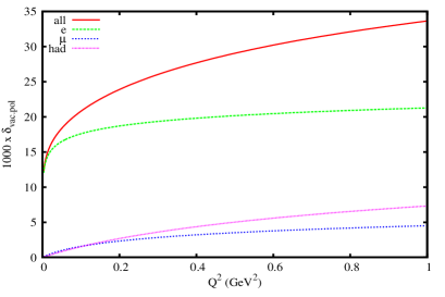
Figure 1: Vacuum polarization corrections due to electrons ($e$), muons ($\mu$), hadrons (had), and the combined effect (all).

Fig. 2 shows the difference between the corrections due to vacuum polarization by electron and muons between the result obtained with the help of the Fortran package alphaQED (taking into account also known 2-loop contributions) and the exponentiated treatment of the effect described in Ref. Bernauer:2013tpr . One can see that the difference is of the order of $2\cdot 10^{4}$ which might be relevant for a better control of systematic errors.

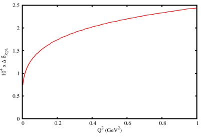
Figure 2: Difference in the leptonic vacuum polarization corrections.

Relative QED corrections to the electron line

$$\delta_{i}=\frac{{\mathrm{d}}\sigma^{(i)}}{{\mathrm{d}}\sigma^{(0)}}$$ (19)

are presented in Fig. 3. Index $i$ runs over:
a) “2,LLA”, i.e. pure photonic ${\mathcal{O}}\left(\alpha^{2}L^{2}\right)$ corrections from Eq. (2.4),
b) “2,NLA”, i.e. the sum of pure photonic ${\mathcal{O}}\left(\alpha^{2}L^{2}\right)$ and ${\mathcal{O}}\left(\alpha^{2}L^{1}\right)$ corrections from Eq. (2.4),
c) “pair”, i.e. the leading log pair corrections from Eq. (2.3) supplemented by subleading pair corrections extracted from Eq. (2.4),
d) “diff.”, i.e. the shift from the exponentiated one-loop result:

$$\delta_{\mathrm{diff.}} = \frac{{\mathrm{d}}\sigma^{\mathrm{NLO}}}{{\mathrm{d}}\sigma^{(0)}(1)}+\delta^{(3)}_{\mathrm{LLA}}+\delta^{(3)}_{\mathrm{LLA,pair}}+\delta^{(4)}_{\mathrm{LLA}}$$ (20)

$$- \exp\{\delta^{(1)}\}.$$

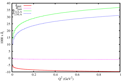
Figure 3: Relative higher order QED corrections to electron line in $ep$ scattering cross section vs momentum transferred squared.

4 Conclusions

In this way we presented results for higher order corrections to elastic electron-proton scattering which can be relevant for modern high-accuracy experiments. The corrections are presented in an analytic form. Numerical results are given for a simplified experimental set-up just to estimate the magnitude of effects. Matching with exponentiated representation of corrections is straightforward, since we have explicit results for sub-leading corrections.

Quantity (20) plotted in Fig. 3 is an estimate of the effect due to an advanced treatment of higher order corrections to the electron line in the process of $ep$ scattering, which is presented here. We have shown also that accurate treatment of vacuum polarization effects is also important for getting a high precision. An adequate treatment of all other relevant effects (double photon exchange, radiative corrections to the proton line, details of the experimental set-up, etc.) is also required.

- (1) J. C. Bernauer et al. [A1 Collaboration], Phys. Rev. C 90 (2014) 1, 015206 [arXiv:1307.6227 [nucl-ex]].
- (2) A. Antognini, F. Nez, K. Schuhmann, F. D. Amaro, FrancoisBiraben, J. M. R. Cardoso, D. S. Covita and A. Dax et al., Science 339 (2013) 417.
- (3) F. A. Berends, W. L. van Neerven and G. J. H. Burgers, Nucl. Phys. B 297 (1988) 429 [Erratum-ibid. B 304 (1988) 921].
- (4) A. Arbuzov and K. Melnikov, Phys. Rev. D 66 (2002) 093003 [hep-ph/0205172].
- (5) A. Arbuzov, JHEP 0303 (2003) 063 [hep-ph/0206036].
- (6) A. B. Arbuzov, D. Haidt, C. Matteuzzi, M. Paganoni and L. Trentadue, Eur. Phys. J. C 34 (2004) 267 [hep-ph/0402211].
- (7) D. R. Yennie, S. C. Frautschi and H. Suura, Annals Phys. 13 (1961) 379.
- (8) A. B. Arbuzov, E. A. Kuraev and B. G. Shaikhatdenov, Mod. Phys. Lett. A 13 (1998) 2305 [hep-ph/9806215].
- (9) E.A. Kuraev and V.S. Fadin, Sov. J. Nucl. Phys. 41 (1985) 466.
- (10) A.B. Arbuzov and E. S. Scherbakova, JETP Lett. 83 (2006) 427 [hep-ph/0602119].
- (11) M. Skrzypek, Acta Phys. Polon. B 23 (1992) 135.
- (12) A.B. Arbuzov, Phys. Lett. B 470 (1999) 252 [hep-ph/9908361].
- (13) F. Jegerlehner, Nuovo Cim. C 034S1 (2011) 31 [arXiv:1107.4683 [hep-ph]].
- (14) A. B. Arbuzov, JHEP 0107 (2001) 043 [hep-ph/9907500].
- (15) J. Arrington, P. G. Blunden and W. Melnitchouk, Prog. Part. Nucl. Phys. 66 (2011) 782 [arXiv:1105.0951 [nucl-th]].
- (16) G. Lee, J. R. Arrington and R. J. Hill, Phys. Rev. D 92 (2015) 1, 013013 [arXiv:1505.01489 [hep-ph]].