Triangular Alignment (TAME):
A Tensor-based Approach for
Higher-order Network Alignment

Abstract

Network alignment has extensive applications in comparative interactomics. Traditional approaches aim to simultaneously maximize the number of conserved edges and the underlying similarity of aligned entities. We propose a novel formulation of the network alignment problem that extends topological similarity to higher-order structures and provides a new objective function that maximizes the number of aligned substructures. This objective function corresponds to an integer programming problem, which is NP-hard. Consequently, we identify a closely related surrogate function whose maximization results in a tensor eigenvector problem. Based on this formulation, we present an algorithm called Triangular AlignMEnt (TAME), which attempts to maximize the number of aligned triangles across networks. Using a case study on the NAPAbench dataset, we show that triangular alignment is capable of producing mappings with high node correctness. We further evaluate our method by aligning yeast and human interactomes. Our results indicate that TAME outperforms the state-of-art alignment methods in terms of conserved triangles. In addition, we show that the number of conserved triangles is more significantly correlated, compared to the conserved edge, with node correctness and co-expression of edges. Our formulation and resulting algorithms can be easily extended to arbitrary motifs.

1 Introduction

Modeling cellular machinery as a network of interacting biomolecules provides significant opportunities for understanding and controlling various biological processes. This complex network, or interactome, may include direct relationships among biomolecules, such as physical, regulatory, or signaling interactions, or indirect phenotypic relationships such as epistatic interactions. One common abstraction is a protein-protein interaction network (PPI), which is an undirected graph, where nodes represent proteins and edges encode physical interactions among pairs of proteins. Protein-protein interaction networks are extensively used for modeling and understanding pathways and protein complexes with respect to their organization and function.

Network motifs are one means of identifying organization and function in these networks. A network motif is a connected subgraph that occurs with significantly higher frequency compared to an ensemble of random graphs with the same size and degree distribution. Over-representation of these patterns are hypothesized to be related to their functional significance [1]; and, indeed, network motif analysis uncovers fundamental circuits that are repeatedly used to perform critical functions within the cell. Due to their important role in decoding biological networks, various algorithms have been proposed in literature for network motif detection [2, 3, 4, 5, 6]. These methods have identified key motifs, such as feed forward and feedback cycles in directed networks and triangles in undirected graphs. Furthermore, these motifs are shown to be involved in regulating cell function, as well as influencing global network characteristics [7, 8, 9, 10, 11].

Concurrent with the development of methods for network motif detection, there has been ongoing work on network alignment algorithms for identification of conserved modules across networks. The goal of network alignment is to identify a mapping between nodes of networks that maximizes similarity (as defined by a suitable measure) between mapped entities. These mappings can be used to infer orthologies for unannotated proteins, as well as transferring known biology regarding common pathways, protein complexes, recurring building blocks, and missing interactions. These conserved substructures are important since cellular functions require all of their constituent components (nodes and their interactions) to be conserved. Conversely, conserved modules provide insights into corresponding functional organization [12].

The network alignment problem, unlike its counterpart over sequences, is NP-complete to solve exactly, since in the most generic form it can be reduced to the subgraph isomorphism problem. However, heuristics have been proposed to generate useful answers through various reformulations as well as by incorporating additional data to guide the alignment process. We survey these methods in Section 2 in more detail. An important distinction among alignment methods is their local versus global nature. Local alignment methods aim to identify conserved functional modules between networks, such as signaling pathways and protein complexes, by optimally aligning these substructures. Due to duplication-divergence events, there can be more than one match for each substructure, which makes alignments ambiguous. Global network alignment, on the other hand, aims to identify a one-to-one mapping between all pair of nodes in the input graphs that maximizes similarity of aligned nodes.

In this paper, we introduce a new class of methods based on higher-order network alignment. These methods combine strengths of both global and local network alignment. In this framework, users can define any network motif structure of interest to drive the alignment process. These general structures can be represented through a motif tensor, in which the order of tensor is the same as the size of the given subgraph template. We encode the higher order network alignment using a tensor-based formulation and show that the exact solution to the alignment problem is equivalent to solving a higher-order integer program, which is NP-hard. To optimize this objective function on large networks, we exploit a bijection between the eigenpairs of the motif tensor and a heuristic approximation of the integer program. We can then use the previously proposed SS-HOPM [13] method to identify maximizing dominant eigenpairs of a symmetric tensor, and propose a higher-order alignment method based on this scheme. The motif tensor of the alignment graph can be represented as the Kronecker product of motif tensors for each input graph. This tensor is too large to fit in the memory for typical PPI networks, even for small motifs. We develop a novel implicit kernel for computing the tensor-vector product as the main operator within SS-HOPM. Similar kernels have been previously proposed in the context of computer vision research  [14, 15]; however, we present a highly efficient, motif-centered version that is easily extensible to higher order sub-structures.

Using a case study of triangle motifs, we present a complete algorithm, called Triangular AlignMEnt (TAME). We propose a constrained variant of our algorithm, cTAME, that operates only on a subset of reliable nodes. This method provides better accuracy in cases where sequence similarity scores are highly reliable proxies for the true-positive alignments. We further validate our method and show that it compares favorably to the state-of-art methods for network alignment on both synthetic datasets from NAPAbench [16] and alignment of yeast and human interactomes. Our framework can be easily extended to arbitrary subgraphs and motivates an alternate view to the network alignment problem.

2 Background and previous methods

Based on the alignment strategy, we can generally classify different methods as either local or global alignment techniques. Local alignment aims to identify common substructures corresponding to pathways or protein complexes that are conserved in networks of different species. Local alignments often yield ambiguous mappings, since functional building blocks can have many-to-many relationships. On the other hand, global alignment attempts to find the best overall mapping between the nodes of input graphs that maximizes both functional and topological similarity of aligned nodes, while enforcing the one-to-one constraint. In pairwise alignment, this leads to a unique alignment for each node in the smaller graph to a node in the larger graph. These alignments are unambiguous and can be used to transfer functional orthologies between pairs of proteins, as well as to compute the overall similarity of input graphs.

Local aligners differ in the topology of the substructures they search for, their objective formulation, and search strategy. PathBlast [17, 18] and NetworkBlast [19, 20] are early examples that use a probabilistic scoring function to search for linear paths and clique-like substructures, respectively. Flannick et al. [21] proposed an evolutionarily-motivated scoring function and incorporated known alignments via a supervised learning scheme [22]. Koyuturk et al. [23, 24] instead posed local alignment as a suitably formulated optimization problem in their MaWISh framework. AlignMCL [25] combines input networks to construct an alignment graph and uses the Markov CLustering (MCL) algorithm to partition the alignment graph and identify protein clusters.

Global aligners, on the other hand, aim to find unique node-to-node mappings that maximize a given objective function. IsoRank  [26, 27] and its predecessor IsoRankN [28] are among the early methods in this class. The main idea behind IsoRank is that a pair of nodes corresponds to a good match if the nodes are homologous and their respective neighborhoods are similar. This recursive scheme is then cast as an eigenvalue problem, the solution of which is identified using power method. Later, Kollias et al. [29, 30] proposed methods to speedup similarity computation and matching phases in IsoRank, respectively. GRAphlet-based ALigner (GRAAL) [31] was proposed as the first member in a family of “GRAAL-based methods.” These methods are distinguished by their use of graphlet degrees of nodes, or the number of induced subgraphs with given topology incident on each vertex, as a topological signature for vertices. H-GRAAL is an extension of the GRAAL method that uses the Hungarian algorithm, hence the name H-GRAAL [32], to compute maximum-weight bipartite matching and extract alignments from the node similarity scores. Matching-based Integrative GRAAL (MI-GRAAL) [33] allows simultaneous integration of five different similarity matrices, including similarity of sequences as well as graphlet degrees. Moreover, it uses a novel seed-and-extend matching strategy that is shown to outperform the Hungarian method in terms of alignment quality. C-GRAAL [34] is a “common-neighbors-based” addition to the GRAAL family that introduces additional heuristics to the seed-and-extend matching strategy. It uses the concept of neighborhood densities to choose the best matching pairs to align. Both heuristics proposed in MI-GRAAL and C-GRAAL aim to implicitly maximize the number of aligned/conserved edges using a greedy alignment strategy. Klau et al. [35, 36] formulate the network alignment problem as an integer quadratic problem (IQP) that aims to simultaneously maximize a convex combination of the total number of aligned edges and overall similarity of mapped nodes. They proposed a method, named NATALIE, which uses Lagrangian relaxation to provide a real approximation to the network alignment problem formulated as an IQP. Bayati et al. [37] proposed a message passing algorithm to solve the IQP proposed by Klau et al. by utilizing the sparsity pattern in the sequence similarity search space. More recently, the latest addition to the GRAAL-family, called Lagrangian GRAAL (L-GRAAL) [38], has been proposed. L-GRAAL is similar to previous members in that it uses graphlet degree signatures as a source of topological similarities. However, it uses a seed-and-extend step that is based on the integer programming and Lagrangian relaxation similar to the one proposed in NATALIE.

In addition to the GRAAL-family, many other methods have been developed. GHOST [39] uses a spectral approach that, similar to GRAAL, tries to encode local topology of each node using a signature vector, called the spectral signature. The similarity of nodes is then identified based on the similarity of their spectral signature. GHOST uses local swaps, similar to the ones proposed in PISwap [40], to post-process the final alignment and improve the results. Similarly, MAGNA [41] is an evolutionary algorithm designed to enhance alignments computed by other methods. The method can also be used as an independent aligner by applying it to a random initial population. MAGNA++ [42] is an extension of MAGNA that allows integration of sequence similarities and provides a GUI for MAGNA. More recently, Gong et al. [43] proposed a memetic algorithm-based algorithm for alignment which is similar in nature to MAGNA in that it iteratively updates alignment using evolutionary swapping operators. HubAlign [44] is a recent network aligner that is based on similar concepts as MaWISh [45]. It uses a minimum degree heuristic to identify and align “important” proteins first, and to use them as anchors to locally extend the alignment to the whole network. Mohammadi et al. [46], Clark et al. [47], and Elmsallati et al. [48] provide a comprehensive comparison of these methods.

3 Notations and Terminology

3.1 Graphs and Hypergraphs

Biochemical networks are often modeled as graphs in which vertices (or nodes) represent biomolecules (proteins, genes, etc.) and edges (or arcs) encode pairwise relationships among them. Formally, a graph $\mathit{\mathbf{\boldsymbol{G}}}$ is represented by $\mathit{\mathbf{\boldsymbol{G}}}=(\mathit{V_{G}},\mathit{E_{G}})$, where $\mathit{V_{G}}$ is a finite set of vertices, $\mathit{V_{G}}=\{v_{1},v_{2},\ldots.,v_{n}\}$, and $\mathit{E_{G}}$ is a finite set of edges, denoted by $(v_{i},v_{j})$, such that $\mathit{E_{G}}\subseteq(\mathit{V_{G}}\times\mathit{V_{G}})$. We focus on undirected graphs, where edges define a symmetric relation among graph vertices. A graph can be represented by a matrix $\mathbf{A}_{\mathit{\mathbf{\boldsymbol{G}}}}$ of size $|\mathit{V_{G}}|\times|\mathit{V_{G}}|$, known as the adjacency matrix, in which $\mathbf{A}_{G}(i,j)=1$ when $(v_{i},v_{j})\in\mathit{E_{G}}$. The graph neighborhood for each node $v_{i}$ in the graph, represented by $\mathit{N}_{G}(i)$, is defined as the set of nodes that have an edge with $v_{i}$; formally $\mathit{N}_{G}(i)=\{j\mid(i,j)\in\mathit{E_{G}}\}$. Given a pair of graphs, $\mathit{\mathbf{\boldsymbol{G}}}=(\mathit{V_{G}},\mathit{E_{G}})$ and $\mathit{\mathbf{\boldsymbol{H}}}=(\mathit{V_{H}},\mathit{E_{H}})$, their Kronecker product is a graph with $|V_{G}|\times|V_{H}|$ vertices that are formed by pairs of vertices from $\mathit{\mathbf{\boldsymbol{G}}}$ and $\mathit{\mathbf{\boldsymbol{H}}}$, e.g., $ii^{\prime}$ for $i$ from $\mathit{V_{G}}$ and $i^{\prime}$ from $\mathit{V_{H}}$. and where each edges between nodes $ii^{\prime}$ and $jj^{\prime}$ corresponds to $(i,j)\in E_{G}$ and $(i^{\prime},j^{\prime})\in E_{H}$.

Hypergraphs are natural generalizations of graphs in which the relations among vertices is not restricted to be pairwise. Formally, a hypergraph is defined using the pair $\mathbfcal{G}=(\mathit{V}_{G},\mathcal{E}_{G})$, where $\mathit{V}$ is the set of vertices and $\mathcal{E}$ is the set of hyperedges. Here, each hyperedge defines a relationship among a nonempty subset of vertices. A $k$-uniform hypergraph is a hypergraph in which the cardinality of each hyperedge is exactly $k$. As such, 2-uniform hypergraphs are equivalent to traditional graphs. A $k$-uniform hypergraph can be represented by a $k^{th}$-order tensor $\mathbf{\mathcal{T}}_{G}$, known as the adjacency tensor, where $\mathbf{\mathcal{T}}_{G}(i_{1},i_{2},\ldots,i_{k})=1$ iff $(i_{1},i_{2},\ldots,i_{k})\in\mathcal{E}_{G}$. The hypergraph incidence set for each node $v_{i}$ in a $k$-uniform hypergraph, represented by $\mathcal{N}_{G}(i)$, is the set of $(k-1)$-node subsets such that adding node $i$ to each subset forms an edge. This is one possible generalization of a neighborhood to a hypergraph, and is formally defined as $\mathcal{N}_{G}(i)=\{(i_{2},i_{3},\ldots,i_{k})\mid(i,i_{2},i_{3},\ldots,i_{k})\in\mathcal{E}_{G}\}$. For a given graph $\mathit{\mathbf{\boldsymbol{G}}}=(\mathit{V_{G}},\mathit{E_{G}})$ and a given size $k$ structural motif $\mathit{\mathbf{\boldsymbol{M}}}=(\mathit{V_{M}},\mathit{E_{M}})$, where $|\mathit{V_{M}}|=k$, we can represent the occurrences of $\mathit{\mathbf{\boldsymbol{M}}}$ in $\mathit{\mathbf{\boldsymbol{G}}}$ by a $k$-way tensor $\mathbf{\mathcal{T}}_{G}$, referred to as the motif-tensor, where $\mathbf{\mathcal{T}}_{G}(i_{1},\ldots,i_{k})=1$ when the induced subgraph among vertices $\{v_{i_{1}},\ldots,v_{i_{k}}\}$ in $\mathit{\mathbf{\boldsymbol{G}}}$ is isomorphic to $\mathit{\mathbf{\boldsymbol{M}}}$. Throughout this paper, we make extensive use of a special case of the motif-tensor where the substructure of interest is the triangle motif. Given an undirected graph $\mathit{\mathbf{\boldsymbol{G}}}$, its triangle tensor, denoted by $\mathbf{\mathcal{\bigtriangleup}}_{G}$, is a third-order tensor such that $\mathbf{\mathcal{\bigtriangleup}}_{G}(i,j,k)=1$ iff $(v_{i},v_{j}),(v_{j},v_{k}),(v_{k},v_{i})\in\mathit{E}_{G}$.

3.2 Tensor definition and properties

A real-valued $m^{th}$-order $n$-dimensional tensor, denoted by $\mathbf{\mathcal{T}}^{[m,n]}$, is a multiway array, whose entries can be indexed using an $m$-dimensional tuple, and each tensor way (or mode) has dimension $n$. An $n$-dimensional vector and square matrix are examples of $1^{st}$-order and $2^{nd}$-order tensors, respectively. We refer to elements of a tensor $\mathbf{\mathcal{T}}^{[m,n]}$ using $\mathbf{\mathcal{T}}(i_{1},i_{2},\ldots,i_{m})$ and $\mathbf{\mathcal{T}}_{i_{1},i_{2},\ldots,i_{m}}$, interchangeably. A tensor $\mathbf{\mathcal{T}}$ is symmetric iff:

$$\mathbf{\mathcal{T}}(i_{1},i_{2},\ldots,i_{m})=\mathbf{\mathcal{T}}(i_{\pi(1)},i_{\pi(2)},\ldots,i_{\pi(m)})$$ (1)

for all $\pi\in\Pi_{m}$, where $\Pi_{m}$ is the set of all permutations of $(1,2,\ldots,m)$. As an example, note that the triangle tensor is a symmetric tensor.

Given a symmetric tensor $\mathbf{\mathcal{T}}^{[m,n]}$, together with an $n$-dimensional vector $\boldsymbol{x}\in\mathbb{R}^{n}$, we concern ourselves with two operations. The first is the tensor-vector product: $\mathbf{\mathcal{T}}\boldsymbol{x}^{m-1}$, which is defined element-wise as

$$(\mathbf{\mathcal{T}}\boldsymbol{x}^{m-1})_{i_{1}}=\sum_{i_{2}=1}^{n}\sum_{i_{3}=1}^{n}\cdots\sum_{i_{m}=1}^{n}\mathbf{\mathcal{T}}_{i_{1},i_{2},\ldots,i_{m}}x_{i_{2}}x_{i_{3}}\ldots x_{i_{m}}.$$ (2)

The second is the scalar polynomial form in $\boldsymbol{x}$: $\mathbf{\mathcal{T}}\boldsymbol{x}^{m}$ defined as

$$\mathbf{\mathcal{T}}\boldsymbol{x}^{m}=\sum_{i_{1}=1}^{n}\sum_{i_{2}=1}^{n}\sum_{i_{3}=1}^{n}\cdots\sum_{i_{m}=1}^{n}\mathbf{\mathcal{T}}_{i_{1},i_{2},\ldots,i_{m}}x_{i_{1}}x_{i_{2}}x_{i_{3}}\ldots x_{i_{m}}.$$ (3)

Note that $\boldsymbol{x}^{T}(\mathbf{\mathcal{T}}\boldsymbol{x}^{m-1})=\mathbf{\mathcal{T}}\boldsymbol{x}^{m}$.

A pair $(\lambda,\boldsymbol{x})$, $\lambda\in\mathbb{R},\boldsymbol{x}\in\mathbb{R}^{n}$, is the Z-eigenpair of the symmetric tensor $\mathbf{\mathcal{T}}$ when:

$$\mathbf{\mathcal{T}}\boldsymbol{x}^{m-1}=\lambda\boldsymbol{x};\text{ with }\|\boldsymbol{x}\|_{2}=1.$$ (4)

Any eigenpair $(\lambda,\boldsymbol{x})$ of tensor $\mathbf{\mathcal{T}}$ is a Karush-Kuhn-Tucker (KKT) point of the following nonlinear optimization problem [49]:

$$\begin{array}[]{ll}\displaystyle\mathop{\text{maximize}}_{\boldsymbol{x}\in\mathbb{R}^{n}}&\mathbf{\mathcal{T}}\boldsymbol{x}^{m}\\ \text{subject to}&\|\boldsymbol{x}\|_{2}=1.\end{array}$$ (5)

We will use one additional concept: the Kronecker product of tensors. This type of product is a reshaped version of the well-established outer product for tensors. Formally, given a pair of symmetric tensors, $\mathbf{\mathcal{T}}_{1}\in\mathcal{R}^{[m,n_{1}]},\mathbf{\mathcal{T}}_{2}\in\mathcal{R}^{[m,n_{2}]}$, their Kronecker product, denoted by $\mathbf{\mathcal{T}}_{1}\otimes\mathbf{\mathcal{T}}_{2}\in\mathcal{R}^{[m,n_{1}n_{2}]}$, is defined as:

$$(\mathbf{\mathcal{T}}_{1}\otimes\mathbf{\mathcal{T}}_{2})(i_{1}i_{1}^{\prime},\ldots,i_{m}i_{m}^{\prime})=\mathbf{\mathcal{T}}_{1}(i_{1},\ldots,i_{m})\mathbf{\mathcal{T}}_{2}(i_{1}^{\prime},\ldots,i_{m}^{\prime})$$ (6)

with $1\leq i_{1},\ldots,i_{m}\leq n_{1}$, $1\leq i_{1}^{\prime},\ldots,i_{m}^{\prime}\leq n_{2}$, and the notation $i_{k}i^{\prime}_{k}$ denotes a specific index for the index representing the pair which is $(i_{k}-1)n_{2}+i^{\prime}_{k}$.

4 Higher-Order Network Alignment

Our framework for higher-order network alignment draws heavily on the integer quadratic program for global network alignment. We begin by reviewing this formulation [50, 35, 36].

4.1 Formulation of global network alignment as a Binary Quadratic Program (BQP)

Given a pair of networks, represented by $\mathit{\mathbf{\boldsymbol{G}}}=(\mathit{V}_{G},\mathit{E}_{G})$ and $\mathit{\mathbf{\boldsymbol{H}}}=(\mathit{V}_{H},\mathit{E}_{H})$, the global network alignment problem aims to find an optimal one-to-one mapping between vertices of $\mathit{\mathbf{\boldsymbol{G}}}$ and $\mathit{\mathbf{\boldsymbol{H}}}$ that maximizes both the prior (known) similarity and the topological similarity among pairs of aligned nodes. The topological similarity is the number of edges preserved in both $\mathit{\mathbf{\boldsymbol{G}}}$ and $\mathit{\mathbf{\boldsymbol{H}}}$ under the matching.

Let us denote by $\boldsymbol{w}(ii^{\prime})$ the prior similarity of a pair of nodes $i\in\mathit{V}_{\mathit{\mathbf{\boldsymbol{G}}}}$ and $i^{\prime}\in\mathit{V}_{\mathit{\mathbf{\boldsymbol{H}}}}$. Here, $ii^{\prime}$ is a shorthand for the linear index $(i^{\prime}-1)|\mathit{V}_{\mathit{\mathbf{\boldsymbol{G}}}}|+i$. (For more detail about this derivation, please see [50].) Furthermore, we use a binary indicator vector $\boldsymbol{x}$ to represent matches, where $\boldsymbol{x}(ii^{\prime})$ is one if node $i$ is matched to node $i^{\prime}$, and zero otherwise. Finally, we define a binary matrix $\mathbf{S}$, where $\mathbf{S}(ii^{\prime},jj^{\prime})$ is one if $(i,j)\in\mathit{E}_{\mathit{\mathbf{\boldsymbol{G}}}}$ and $(i^{\prime},j^{\prime})\in\mathit{E}_{\mathit{\mathbf{\boldsymbol{H}}}}$, and zero otherwise. For the choice of $ii^{\prime}$ listed above, $\mathbf{S}=A_{\mathit{\mathbf{\boldsymbol{H}}}}\otimes A_{\mathit{\mathbf{\boldsymbol{G}}}}$. Using this notation, we can write the global network alignment as the following binary quadratic program (BQP):

$$\begin{array}[]{ll}\displaystyle\mathop{\text{maximize}}_{\boldsymbol{x}}&\displaystyle(1-\alpha)\boldsymbol{w}^{T}\boldsymbol{x}+\frac{\alpha}{2}\boldsymbol{x}^{T}\mathbf{S}\boldsymbol{x}\\ \text{subject to}&\mathbf{C}\boldsymbol{x}\leq\boldsymbol{1}_{|V_{G}|+|V_{H}|}\\ &\boldsymbol{x}(ii^{\prime})\in\{0,1\}.\end{array}$$ (7)

where $\mathbf{C}$ is the unsigned node-edge incidence matrix of the complete bipartite graph on $|V_{G}|$ and $|V_{H}|$ vertices. This problem is also equivalent to a binary linear program through a standard linearizing transformation [35, 50]. Different global alignment methods can be viewed as algorithms that either implicitly or explicitly optimize this BQP formulation.

4.2 The higher-order generalization

We generalize the node alignment solutions proposed earlier to the problem of aligning higher-order substructures in graphs. As previously mentioned, this is motivated by the existence of motifs in biological networks. Again, we will use vectors whose indices represent pairs $ii^{\prime}$ as above. Let $\mathbf{\mathcal{T}}_{G}$ and $\mathbf{\mathcal{T}}_{H}$ be the motif-tensors associated with a motif $\mathit{\mathbf{\boldsymbol{M}}}$ in both graphs $G$ and $H$, where this motif has $m$-nodes. Then the higher-order network alignment problem is the binary polynomial problem:

$$\begin{array}[]{ll}\displaystyle\mathop{\text{maximize}}_{\boldsymbol{x}}&\displaystyle(1-\alpha)\boldsymbol{w}^{T}\boldsymbol{x}+\frac{\alpha}{m!}(\mathbf{\mathcal{T}}_{H}\otimes\mathbf{\mathcal{T}}_{G})\boldsymbol{x}^{m}\\ \text{subject to}&\mathbf{C}\boldsymbol{x}\leq\boldsymbol{1}_{|V_{G}|+|V_{H}|}\\ &\boldsymbol{x}(ii^{\prime})\in\{0,1\}.\end{array}$$ (8)

This problem can again be converted into a binary linear program through a standard linearization procedure on the higher-order polynomials, but that is tangential to our discussion here. As a generalization of the network alignment problem, this problem is NP-hard as well.

We focus on triangle motifs, which are special cases of feed-forward/backward motifs. Please note that our method is general, and can be applied to arbitrary motifs. Denote the triangle tensor of graph $\mathit{\mathbf{\boldsymbol{G}}}$ and $\mathit{\mathbf{\boldsymbol{H}}}$ using $\mathbf{\mathcal{\bigtriangleup}}_{G}$ and $\mathbf{\mathcal{\bigtriangleup}}_{H}$, respectively. Also, denote the triangle tensor for the product graph by $\mathbf{\mathcal{\bigtriangleup}}_{H\times G}=\mathbf{\mathcal{\bigtriangleup}}_{H}\otimes\mathbf{\mathcal{\bigtriangleup}}_{G}$. Using this notation, we can write the higher-order network alignment problem as a binary cubic program:

$$\begin{array}[]{ll}\displaystyle\mathop{\text{maximize}}_{\boldsymbol{x}}&\displaystyle(1-\alpha)\boldsymbol{w}^{T}\boldsymbol{x}+\frac{\alpha}{6}(\mathbf{\mathcal{\bigtriangleup}}_{H\times G})\boldsymbol{x}^{3}\\ \text{subject to}&\mathbf{C}\boldsymbol{x}\leq\boldsymbol{1}_{|V_{G}|+|V_{H}|}\\ &\boldsymbol{x}(ii^{\prime})\in\{0,1\}.\end{array}$$ (9)

In this formulation, $\mathbf{\mathcal{\bigtriangleup}}_{H\times G}\boldsymbol{x}^{3}$ counts the number of triangles that are conserved under the alignment represented by vector $\boldsymbol{x}$, and $\boldsymbol{w}^{T}\boldsymbol{x}$ plays a similar role as in BQP formulation of global alignment.

We propose a heuristic procedure to optimize this objective. First, we remove the one-to-one constraint on $\boldsymbol{x}$ from the optimization problem. Second, we relax the the problem over the reals. In this case, the solution is unbounded. So we introduce a 2-norm constraint on the solution vector $\boldsymbol{x}$. When $\alpha=1$, then the resulting problem coincides with the eigenvectors of tensor $\mathbf{\mathcal{\bigtriangleup}}_{H\times G}$, as presented in Equation 5. Specifically, the surrogate we use is:

$$\begin{array}[]{ll}\displaystyle\mathop{\text{maximize}}_{\boldsymbol{x}}&(\mathbf{\mathcal{\bigtriangleup}}_{H\times G})\boldsymbol{x}^{3}\\ \text{subject to}&\|\boldsymbol{x}\|=1.\end{array}$$ (10)

For this problem, there is a known algorithm, called shifted symmetric higher-order power method (SS-HOPM) [13], which can be used to identify eigenpairs of $\mathbf{\mathcal{\bigtriangleup}}_{H\times G}$ with large eigenvalues. When $\alpha$ is not 1, we still compute the same tensor eigenvector. We incorporate sequence similarities encoded by $\boldsymbol{w}$ by starting iterations from $\boldsymbol{x}_{0}=\boldsymbol{w}$. Finally, we take the real-valued solution from SS-HOPM and form a matrix $\mathbf{X}(i,i^{\prime})=\boldsymbol{x}(ii^{\prime})$ that we will post-process to produce a 1-1 matching.

We now describe a number of ways to exploit the structure of the problem in this setup for a more efficient implementation. The fundamental computational difficulty is manipulating the tensor $\mathbf{\mathcal{\bigtriangleup}}_{H\times G}$. A straightforward application of SS-HOPM on this tensor would utilize a data structure that consumes 55 TB of memory (this exploits sparsity alone, like traditional graph algorithms). To see how this structure balloons in size, consider the case of aligning the yeast and human interactomes. These networks have $347,079$ and $407,650$ triangles, respectively. If we store the non-zeros in a sparse tensor representation of $\mathbf{\mathcal{\bigtriangleup}}_{H\times G}$ using three 32-bit indices per non-zero, it requires (347,079$~{}\times~{}$ 407,650 motifs)$~{}\times~{}$(36 symmetry non-zeros per motif)$~{}\times~{}$(12 bytes per non-zero)$~{}\approx~{}$55.5 terabytes of memory to store the product tensor ( or 1.5 terabytes, if we exploit the symmetry). Forming the full non-zero structure, however, is unnecessary as we only need to use this tensor to compute the tensor-times-vector operation. This can be done implicitly without forming the complete structure, which is discussed in Section 4.3.

4.3 An implicit kernel for computing tensor-vector products

The key challenge in computing the tensor-vector product is that the number of elements in the triangle tensor of product graph, $\mathbf{\mathcal{\bigtriangleup}}_{H\times G}$, is too large to fit in the memory of most modern computers, even for relatively small graphs. To remedy this problem, we note that there is no need to explicitly construct $\mathbf{\mathcal{\bigtriangleup}}_{H\times G}$. All we need to run SS-HOPM is to compute $\mathbf{\mathcal{\bigtriangleup}}_{H\times G}\boldsymbol{x}^{3}$ and $\mathbf{\mathcal{\bigtriangleup}}_{H\times G}\boldsymbol{x}^{2}$. Re-writing the tensor-vector product formulation in Equation 2, we find the following vertex-centered, implicit kernel as follows:

$$(\mathbf{\mathcal{\bigtriangleup}}_{H\times G}\boldsymbol{x}^{2})_{ii^{\prime}}$$ (11)

$$\quad=\sum_{\mathclap{jj^{\prime},kk^{\prime}}}\mathbf{\mathcal{\bigtriangleup}}_{H\times G}(ii^{\prime},jj^{\prime},kk^{\prime})\boldsymbol{x}(jj^{\prime})\boldsymbol{x}(kk^{\prime})$$

$$\quad=\sum_{\mathclap{j,j^{\prime},k,k^{\prime}}}\mathbf{\mathcal{\bigtriangleup}}_{G}(i,j,k)\mathbf{\mathcal{\bigtriangleup}}_{H}(i^{\prime},j^{\prime},k^{\prime})\mathbf{X}(j,j^{\prime})\mathbf{X}(k,k^{\prime})$$

$$\quad=\sum_{\mathclap{j,k}}\mathbf{\mathcal{\bigtriangleup}}_{G}(i,j,k)\sum_{j^{\prime}}\mathbf{X}(j,j^{\prime})\sum_{k^{\prime}}\mathbf{\mathcal{\bigtriangleup}}_{H}(i^{\prime},j^{\prime},k^{\prime})\mathbf{X}(k,k^{\prime})$$

where $\mathbf{X}=\textbf{unvec}(\boldsymbol{x})$. Additionally, we can simplify this vertex-centered formulation to derive a more efficient motif-centered kernel. To this end, we note that triangle tensors of graphs $\mathit{\mathbf{\boldsymbol{G}}}$ and $\mathit{\mathbf{\boldsymbol{H}}}$ represent a 3-uniform hypergraph over the set of vertices $V_{G}$ and $V_{H}$, respectively. Denote the hypergraph incidences of these hypergraphs by $\mathcal{N}_{\bigtriangleup_{G}}$ and $\mathcal{N}_{\bigtriangleup_{H}}$, where $\mathcal{N}_{\bigtriangleup_{G}}(i)=\{(j,k)\mid(v_{i},v_{j}),(v_{j},v_{k}),(v_{k},v_{i})\in\mathit{E}_{G}\}$, and $\mathcal{N}_{\bigtriangleup_{H}}(i^{\prime})=\{(j^{\prime},k^{\prime})\mid(v_{i^{\prime}},v_{j^{\prime}}),(v_{j^{\prime}},v_{k^{\prime}}),(v_{k^{\prime}},v_{i^{\prime}})\in\mathit{E}_{H}\}$. Then

$$\mathbf{\mathcal{\bigtriangleup}}_{H\times G}\boldsymbol{x}^{2}(ii^{\prime})=$$ (12)

$$\qquad 2\sum_{\mathclap{(j,k)\in\mathcal{N}_{\bigtriangleup_{G}}(i)}}\textstyle\sum_{(j^{\prime},k^{\prime})\in\mathcal{N}_{\bigtriangleup_{H}}(i^{\prime})}\scriptstyle\mathbf{X}(j,j^{\prime})\mathbf{X}(k,k^{\prime})+\mathbf{X}(j,k^{\prime})\mathbf{X}(k,j^{\prime}).$$

In this formulation, we make use of the symmetric property of triangle tensors, where the outer factor of $2$ corresponds to the $(m-1)$ degrees of symmetries. The inner summation accounts for the fact that nodes $v_{j}$ and $v_{k}$ from $\mathit{\mathbf{\boldsymbol{G}}}$, or vertices $\{v_{i_{2}},\ldots,v_{i_{k}}\}$ when dealing with motif-tensors of size $k$, can be mapped to their counterpart vertices $v_{j^{\prime}}$ and $v_{k^{\prime}}$ in $\mathit{\mathbf{\boldsymbol{H}}}$ in $(m-1)!$ different ways. Each of these mappings contribute a factor of one in $\mathbf{\mathcal{\bigtriangleup}}_{H\times G}$. However, their corresponding $\boldsymbol{x}$ values are different and we need to separately compute their product. We use this motif-centered formulation in our final algorithm to compute the implicit tensor-kernel product, $\tilde{\boldsymbol{x}}=\mathbf{\mathcal{\bigtriangleup}}_{H\times G}\boldsymbol{x}^{2}$. Having $\tilde{\boldsymbol{x}}$, one can easily compute $\mathbf{\mathcal{\bigtriangleup}}_{H\times G}\boldsymbol{x}^{3}=\boldsymbol{x}^{T}\tilde{\boldsymbol{x}}$. The simplified pseudo-code of the implicit kernel for computing $\mathbf{\mathcal{\bigtriangleup}}_{G\times H}\boldsymbol{x}^{2}$ is provided in Algorithm 1. The computation time of this algorithm is of $O(|{\bigtriangleup}_{G}|\times|{\bigtriangleup}_{H}|)$.

0:  Triangle-tensors ${\bigtriangleup}_{G},\mathbf{\mathcal{\bigtriangleup}}_{H}$, for $\mathit{\mathbf{\boldsymbol{G}}}$ and $\mathit{\mathbf{\boldsymbol{H}}}$; a vector $\boldsymbol{x}$

0:  $\boldsymbol{y}=\mathbf{\mathcal{\bigtriangleup}}_{H\times G}\boldsymbol{x}^{2}$

1:  $\mathbf{X}=\textbf{unvec}(\boldsymbol{x})$

2:  $\mathbf{Y}=\mathbf{0}$

3:  for $v_{i}\in V_{G}$ do

4:     for $v_{i^{\prime}}\in V_{H}$ do

5:        for $\{(j,k)\in\mathit{N}_{\bigtriangleup_{G}}(i)\}$ do

6:           for $\{(j^{\prime},k^{\prime})\in\mathit{N}_{\bigtriangleup_{H}}(i^{\prime})\}$ do

7:              $\mathbf{Y}(i,i^{\prime})\mbox{{+=}}\mathbf{X}(j,j^{\prime})\mathbf{X}(k,k^{\prime})+\mathbf{X}(j,k^{\prime})\mathbf{X}(k,j^{\prime})$

8:           end for

9:        end for

10:        $\mathbf{Y}(i,i^{\prime})=\mathbf{Y}(i,i^{\prime})*2$

11:     end for

12:  end for

13:  $\boldsymbol{y}=\textbf{vec}(\mathbf{Y})$

Algorithm 1 Implicit tensor-times-vector product (impTTV)

4.4 Triangular AlignMEnt (TAME) algorithm

We now integrate different building blocks introduced earlier to present a higher-order alignment method for triangle motifs. This code uses one additional primitive. The function score solves a bipartite maximum-weight matching problem (using the Hungarian method) and returns the total number of triangles $t$ aligned by the matching. The pseudocode for TAME algorithm is presented in Algorithm 2.

0:  Triangle tensors $\mathbf{\mathcal{\bigtriangleup}}_{G},\mathbf{\mathcal{\bigtriangleup}}_{H}$; Sequence similarities $\boldsymbol{w}$; Shift parameter $\beta$

0:  The best topological scores $\mathbf{X}$ from any iteration

1:  $k=0$ {Iteration number}

2:  $\boldsymbol{w}\leftarrow\boldsymbol{w}/\|\boldsymbol{w}\|$

3:  $\boldsymbol{x_{0}}=\boldsymbol{w}$

4:  $t_{0}=0$

5:  repeat

6:     $\tilde{\boldsymbol{x}}_{k+1}=\textbf{impTTV}(\mathbf{\mathcal{\bigtriangleup}}_{G},\mathbf{\mathcal{\bigtriangleup}}_{H},\boldsymbol{x}_{k})$

7:     $\lambda_{k+1}=\boldsymbol{x}_{k}^{T}\tilde{\boldsymbol{x}}_{k+1}$

8:     $\hat{\boldsymbol{x}}_{k+1}=\tilde{\boldsymbol{x}}_{k+1}+\beta\boldsymbol{x}_{k}$

9:     $\boldsymbol{x}_{k+1}=\frac{\hat{\boldsymbol{x}}_{k+1}}{\|\hat{\boldsymbol{x}}_{k+1}\|}$

10:     $\mathbf{X}_{k+1}=\bf{unvec}(\boldsymbol{x}_{k+1})$

11:     $t_{k+1}=\bf{score}(\mathbf{X}_{k+1})$

12:     Update $(\mathbf{X},t)_{\text{best}}$ to $(\mathbf{X},t)_{k+1}$ if $t_{k+1}>t_{\text{best}}$

13:     $k=k+1$

14:  until $\lambda_{k}-\lambda_{k-1}$ is small or the max iteration is hit

15:  return  $\mathbf{X}_{\text{best}}$

Algorithm 2 The Triangular AlignMEnt (TAME) algorithm

The overall algorithm takes in the prior similarity and uses that to initialize the SS-HOPM (lines 5-14). impTTV procedure uses the motif-centered, implicit tensor-times-vector kernel proposed in Section 4.3. The SS-HOPM main loop generates a sequence of topological similarity matrices. However, the SS-HOPM process generates a sequence to optimize the problem after removing the two constraints in Equation 9, namely the integer constraint on $\boldsymbol{x}$ and the one-to-one matching constraint over $\mathbf{X}$. To enforce these constraints, we perform a matching in each iteration and compute topological score as the total number of aligned triangles. We keep the highest scoring topological matrix as $\mathbf{X}_{\text{best}}$.

In addition to Algorithm 2, which we refer to as full TAME, we present a variant of this algorithm, called constrained TAME, which only matches nodes that have at least one match suggested by the prior alignment. In this formulation, we must update $\mathbf{\mathcal{\bigtriangleup}}_{G}$ and $\mathbf{\mathcal{\bigtriangleup}}_{H}$ prior to running the full TAME algorithm. The key idea is to remove triangles for which at least one of the end-points has no homology suggested by the sequence similarity. This allows us to focus on the most promising regions of the graph. The constrained TAME method is presented in Algorithm 3. In this algorithm, we first compute a pair of indicator vectors, $\boldsymbol{w}_{r}$ and $\boldsymbol{w}_{c}$ with size $|\mathit{V}_{G}|$ and $|\mathit{V}_{H}|$, respectively. Each element $i$ in $\boldsymbol{w}_{r}$ indicates if vertex $v_{i}\in\mathit{V}_{G}$ has at least one homolog among vertices of $\mathit{\mathbf{\boldsymbol{H}}}$ and, similarly, each element $i^{\prime}$ in $\boldsymbol{w}_{c}$ indicates if vertex $v_{i^{\prime}}\in\mathit{V}_{H}$ has at least one homolog among vertices of $\mathit{\mathbf{\boldsymbol{G}}}$ (determined by the prior similarity). The “.*” operator is the element-wise product of two tensors. Finally, we prune the triangle tensors by enforcing that all end-points of every triangle motif should have at least one homolog in the other graph. An equivalent way of understanding this algorithm is that we first remove vertices from $\mathit{\mathbf{\boldsymbol{G}}}$ and $\mathit{\mathbf{\boldsymbol{H}}}$ that have no prior information indicating there is a match in the other graph.

0:  Triangle tensors $\mathbf{\mathcal{\bigtriangleup}}_{G},\mathbf{\mathcal{\bigtriangleup}}_{H}$; Sequence similarities $\boldsymbol{w}$; Shift parameter $\beta$

0:  The final set of aligned node pairs $\langle\boldsymbol{m_{i}},\boldsymbol{m_{i}^{\prime}}\rangle$

1:  $\mathbf{W}=\text{{unvec}}(\boldsymbol{w})$

2:  $\boldsymbol{w}_{G}=\text{indicator vector for rows of $\mathbf{W}$ with non-zeros}$

3:  $\boldsymbol{w}_{H}=\text{indicator vector for cols of $\mathbf{W}$ with non-zeros}$

4:  $\mathbf{\mathcal{W}}_{G}=\boldsymbol{w}_{G}\otimes\boldsymbol{w}_{G}\otimes\boldsymbol{w}_{G}$

5:  $\mathbf{\mathcal{W}}_{H}=\boldsymbol{w}_{H}\otimes\boldsymbol{w}_{H}\otimes\boldsymbol{w}_{H}$

6:  $\mathbf{\mathcal{\bigtriangleup}}_{G}^{(\text{contrained})}=\mathbf{\mathcal{\bigtriangleup}}_{G}.*\mathbf{\mathcal{W}}_{G}$

7:  $\mathbf{\mathcal{\bigtriangleup}}_{H}^{(\text{contrained})}=\mathbf{\mathcal{\bigtriangleup}}_{H}.*\mathbf{\mathcal{W}}_{H}$

8:  $\mathbf{X}=\textbf{TAME}(\mathbf{\mathcal{\bigtriangleup}}_{G}^{(\text{contrained})},\mathbf{\mathcal{\bigtriangleup}}_{H}^{(\text{contrained})},\boldsymbol{w},\beta)$

Algorithm 3 The contrained Triangular AlignMEnt (cTAME) algorithm

This algorithm has the side-effect of reducing the total number of triangles (see Table II), resulting in a faster execution time. In many cases, it also outperforms the full version of TAME in terms of alignment quality by focusing the search in more promising regions. We discuss the pros and cons of each of these methods in Section 5

4.5 Post-processing algorithm

The result matrix $\mathbf{X}$ returned by both TAME and cTAME is a heuristic for the integer problem (9) since it is real-valued and it does not enforce a one-to-one constraint during its iterations. We propose a post-processing step, presented in Algorithm 4, that aims to maximize the objective (9) in the process of generating an integer solution from $\mathbf{X}$. The overarching idea of the post-processing algorithm is to examine small regions around each matched pair to find a local swap that either enhances topological similarity or preserves topological similarity and improves sequence similarity. These principles are similar to PISwap [40] and GHOST [39] in that we swap matches using a greedy approach to enhance the overall quality of the alignment. Given a matching $M$, we define the sequence similarity as $\sum_{ii^{\prime}\in M}w(i,i^{\prime})$ and the topological similarity as $\sum_{ii^{\prime},jj^{\prime},kk^{\prime}\in M}\Delta_{G}(i,j,k)\Delta_{H}(i^{\prime},j^{\prime},k^{\prime})[1+\max(w(jj^{\prime})+w(kk^{\prime}),w(jk^{\prime})+w(kj^{\prime}))]$. Intuitively, this can be seen as a weighted average of triangles incident on each aligned pair $ii^{\prime}$, which encourages additional sequence similarity. These are the two components we evaluate each time we consider a local swap and use the rule above to accept the swap.

The way we implement the iterative swapping procedure is as follows. We begin post-processing by using the Hungarian algorithm to identify a max-weight bipartite matching on the TAME matrix $\mathbf{X}$. Then, we consider a fixed number of rounds of swapping. At the start of each round, we build a list of unprocessed matches based on the current matching that exists at that point in time. This list is examined in order of largest weighted degree of the matched vertices in the bipartite graph with matrix $\mathbf{X}$ in order to increase the likelihood of a swap. In each examination step, we consider a match $ii^{\prime}$ and search for possible swaps within its local neighborhood (defined next) that increase quality. We then evaluate each potential swap and accept it if it increases the topological similarity or preserves the topological similarity and increases sequence similarity. At the end, if we decided to swap $ii^{\prime}$ and $jj^{\prime}$, then we implement the swap in the matching immediately and update $jj^{\prime}$ to $ji^{\prime}$ in the list of unprocessed matches. (There is no re-sorting and this may be effectively ignored if $jj^{\prime}$ was already processed, itself.)

The local neighborhood searched for improved matches consists of a $b$-matching over the $\mathbf{X}$ from TAME and another $b$-matching over the sequence similarity scores. We use a half-approximation algorithm [51] to solve the $b$-matching problem in linear time [52]. Thus, when examining a matched edge, the set of alternative candidates is the union of the neighbors in the $b$-matching of topological scores from $\mathbf{X}$, the neighbors of the $b$-matching of the sequence similarity scores, and the neighbors in the two protein interaction networks ($\mathit{N}_{\mathit{\mathbf{\boldsymbol{H}}}}(i^{\prime})$ and $\mathit{N}_{\mathit{\mathbf{\boldsymbol{G}}}}(i)$). These local alternative sets are called preferred sets [40] and $\text{Pref}_{H}(i)$ and $\text{Pref}_{G}(i^{\prime})$ represent alternative matches for $i$ in graph $\mathit{\mathbf{\boldsymbol{H}}}$ and $i^{\prime}$ in graph $\mathit{\mathbf{\boldsymbol{G}}}$, respectively. The set of possible swaps for $ii^{\prime}$ comprise any other pair $jj^{\prime}$ where $j^{\prime}\in\text{Pref}_{H}(i)$ and $j\in\text{Pref}_{G}(i^{\prime})$ and $j$ is already matched to $j^{\prime}$, in which case the swap is $ij^{\prime}$ and $ji^{\prime}$. We also consider a swap $ii^{\prime}$ to $ij^{\prime}$ if $j^{\prime}\in\text{Pref}_{H}(i)$ and $j^{\prime}$ is unmatched (and likewise, $ii^{\prime}$ to $ji^{\prime}$ if $j\in\text{Pref}_{G}(i^{\prime})$ and $j$ is unmatched).

0:  Output matrix of TAME/cTAME $\mathbf{X}$; Sequence similarity matrix $\mathbf{W}$; matching degree for topological scores $b_{topo}$; matching degree for sequence similarities $b_{seq}$

0:  Final alignment $M$

1:  Set the initial matching $M$ based on solving a max-weight matching problem in $\mathbf{X}$

2:  Set $\mathit{M}_{C}$ to the union of a $b_{\text{seq}}$-matching in the sequence similarity $\mathbf{W}$ and a $b_{\text{topo}}$-matching in the matrix $\mathbf{X}$

3:  for a fixed number of iterations do

4:     Sort matches in $\mathit{M}$ based on $\delta_{ii^{\prime}}=\sum_{i}x({ii^{\prime}})+\sum_{i^{\prime}}x({ii^{\prime}})$ and set the unprocessed list $\mathcal{L}$ to these matches

5:     for each unprocessed $ii^{\prime}\in\mathcal{L}$ in the sorted order do

6:        set $ii^{\prime}$ as processed

7:        Set Pref${}_{\mathit{\mathbf{\boldsymbol{H}}}}(i)$ = {j’; $ij^{\prime}\in\mathit{M}_{C}$ or $j^{\prime}\in\mathit{N}_{\mathit{\mathbf{\boldsymbol{H}}}}(i^{\prime})$}

8:        Set Pref${}_{\mathit{\mathbf{\boldsymbol{G}}}}(i^{\prime})$ = {j; $i^{\prime}j\in\mathit{M}_{C}$ or $j\in\mathit{N}_{\mathit{\mathbf{\boldsymbol{G}}}}(i)$}

9:        for each swap $S$ of the match $i$, $i^{\prime}$ with another matched pair $j$,$j^{\prime}$ in the preferred sets or any unmatched vertex in the preferred sets  do

10:           Check if $M$ with swap $S$ results in a higher topological similarity and accept it if it does, also accept if the topological score is equivalent, but the sequence score is higher. (These are defined in the text)

11:        end for

12:        If the final swap $S$ contains a matched pair $j,j^{\prime}$, then update $j,j^{\prime}$ to $j,i^{\prime}$ in $\mathcal{L}$, but do not resort.

13:     end for

14:  end for

15:  return  $\mathit{M}$

Algorithm 4 Post-processing algorithm

5 Results and Discussion

5.1 Datasets

5.1.1 Synthetic Datasets and Random Networks

NAPAbench [16], is a family of random graphs that has been proposed for evaluating network alignment methods on synthetic datasets. This dataset contains both pairs of networks for evaluating pairwise alignment methods, as well as groups of networks for testing multiple alignment algorithms. There are three random graph generation models employed by NAPAbench: (i) duplication-mutation-complementation (DMC), (ii) duplication with random mutation (DMR), and (iii) crystal growth (CG). These random networks mimic key properties of biological graphs, including their network topology and modular structure. We focus on the crystal growth (CG) dataset, which is based on a model that better fits features of real PPI networks, including their characteristic age distribution [53]. This dataset contains 10 pairs of graphs, for which the known orthology and simulated sequence similarities between pairs of nodes are available. Each pair consists of a first graph $A$ with $3,000$ nodes and a second graph $B$ with $4,000$ nodes. These two networks share a common ancestor of size $2,000$ and have been evolved independently after that. Edge and triangle statistics for these graphs are summarized in Table I

TABLE I: Summary statistics for the NAPAbench dataset

	# nodes	Mean # edges	Mean # triangles
Graph A	3,000	11,985	11,362
Graph B	4,000	15,985	15,880

5.1.2 Yeast Versus Human Interactome Dataset

Both yeast and human protein-protein interaction (PPI) networks were constructed from BioGRID database, version 3.2.103. All physical interactions, excluding self-loops and interspecies interactions, have been filtered and mapped to Entrez gene IDs. We used these interaction evidences to construct the adjacency matrix for both graphs. Edge and triangle statistics for each network are presented in Table II.

TABLE II: Summary statistics for yeast and human interactomes.

	# nodes	# edges	# triangles
Human	14,867	126,593	407,650
Yeast	5,850	79,458	347,079
constrained Human	10,624	88,276	251,555
constrained Yeast	5,482	73,739	289,893

We downloaded the protein sequences for the yeast and humans genes in FASTA format from Ensembl database, release 69. These datasets are based on the GRCh37 and EF4 reference genomes, each of which contain 101,075 and 6,692 protein sequences for H. Sapiens and S. Cerevisiae, respectively. Each human gene in this dataset has, on average, around 4 protein isoforms. We identified and masked low-complexity regions in protein sequences using pseg program [54]. The ssearch36 tool, from FASTA [55] version 36, was then used to compute the local sequence alignment of the protein pairs using the Smith-Waterman algorithm [56]. We used this tool with the BLOSUM50 scoring matrix to compute sequence similarity of protein pairs in humans and yeast. All sequences with E-values less than or equal to 10 are recorded as possible matches, which results in a total of 664,769 hits between yeast and human proteins. For genes with multiple protein isoforms, coming from alternatively spliced variants of the same gene, we only record the most significant hit. The final dataset contains 162,981 pairs of similar protein-coding genes. After mapping these pairs to the human and yeast interactomes, we were able to find matches for 127,505 node pairs in these networks.

5.1.3 Tissue-specific gene expression dataset

We downloaded the RNASeq dataset version 4.0 (dbGaP accession phs000424.v4.p1) from the The Genotype-Tissue Expression (GTEx) project [57]. We processed each sample using the UPC [58]. For each gene, we recorded the alternatively spliced transcript with the highest activation probability in the sample. The final dataset contains the expression value of 23,243 genes across 2916 biological samples, which includes 30 different tissues/cell types.

5.2 Evaluation Criteria

For each alignment, we separately assess the topological quality of the alignment graph, as well as the biological relevance of aligned nodes in the input graphs. Additionally, for the NAPAbench synthetic dataset, we use known matches to compute the correctness of network alignment. Measures described here are adopted from a recent work by Meng et al. [59] as general means to compare local versus global network alignments. Specifically, generalized $S^{3}$ (GS3) and F-FP are shown to be good surrogates for topological and biological quality of alignment with respect to edge conservation and gene ontology (GO) consistency. We extend the concept of GS3 to the case of triangles, which we call triangular GS3 (tGS3). In addition, we introduce a new measure based on co-expression of genes to validate biological plausibility of network alignments.

Let $m(ii^{\prime})$ be an indicator function for matching, that is, $m(ii^{\prime})=1$ iff vertex $v_{i}\in V_{G}$ is matched to $v_{i^{\prime}}$ in $V_{H}$. Furthermore, let $\hat{m}(ii^{\prime})$ be an indicator of true alignments, which is one if vertex $i$ in $V_{G}$ is a true match for vertex $i^{\prime}$ in $V_{H}$. Let $\mathit{M}$ and $\mathit{\hat{M}}$ be the set of aligned pairs and true alignments. Using this notation, we can formulate different performance measures are as follows:

5.2.1 Node Correctness (NC)

This measure is only defined for synthetic cases for which the true-alignment is known a priori. We can define precision and recall for each alignment as $P=\frac{|\mathit{M}\cap\mathit{\hat{M}}|}{|\mathit{M}|}$ and $R=\frac{|\mathit{M}\cap\mathit{\hat{M}}|}{|\mathit{\hat{M}}|}$, respectively. Then, the F-score of node correctness, denoted by F-NC, can be computed as the harmonic mean of the precision and recall.

5.2.2 Node Coverage (NCV)

Let us define the “unique” operator that when applied to a list returns the unique elements of the list as a set. We will denote by $V_{\mathit{\mathbf{\boldsymbol{G}}}}^{(A)}$ the set of touched vertices in $\mathit{\mathbf{\boldsymbol{G}}}$ under alignment $A$, which is computed as unique($[i];\forall ii^{\prime}\in\mathit{M}$). $V_{\mathit{\mathbf{\boldsymbol{H}}}}^{(A)}$ can be defined similarly for graph $\mathit{\mathbf{\boldsymbol{H}}}$. Using this notation, NCV can be computed as $\frac{|V_{\mathit{\mathbf{\boldsymbol{G}}}}^{(A)}|+|V_{\mathit{\mathbf{\boldsymbol{H}}}}^{(A)}|}{|V_{\mathit{\mathbf{\boldsymbol{G}}}}|+|V_{\mathit{\mathbf{\boldsymbol{H}}}}|}$.

5.2.3 NCV-Generalized $S^{3}$ (GS3)

We can compute the total number of conserved edges from the edge-set of the alignment graph, i.e. $E_{C}=\{(ii^{\prime},jj^{\prime})\mid(i,j)\in E_{G},(i^{\prime},j^{\prime})\in E_{H},\text{{ and }}m(ii^{\prime})=m(jj^{\prime})=1\}$. Similarly, we can define the set of gapped edges as $E_{\not C}=\{(ii^{\prime},jj^{\prime})\mid(i,j)\in E_{G},(i^{\prime},j^{\prime})\not\in E_{H}\text{{ or }}(i,j)\not\in E_{G},(i^{\prime},j^{\prime})\in E_{H},\text{{ and }}m(ii^{\prime})=m(jj^{\prime})=1\}$. Then, GS3 measure is defined as $\frac{|E_{C}|}{|E_{C}|+|E_{\not}C|}$. For complete one-to-one alignments (each node in smaller graph is mapped to exactly one node in the larger graph), GS3 measure is equivalent to S3 measure. However, GS3 allows comparison with sparse as well as local alignment methods. One downside of GS3 is that it does not penalize for the size of alignment. For example, an alignment that only aligns one conserved edge will have perfect GS3. To remedy this, we compute the geometric mean of NCV and GS3, which is called NCV-GS3 measure.

5.2.4 NCV-Triangular GS3 (tGS3)

Similar to $GS3$, triangular GS3 (tGS3) is defined on the basis of total number of conserved and gaped triangles. It can be represented with respect to the triangle-set of the alignment graph, $T_{C}=\{(ii^{\prime},jj^{\prime},kk^{\prime})\mid(i,j,k)\in T_{G},(i^{\prime},j^{\prime},k^{\prime})\in T_{H},\text{{ and }}m(ii^{\prime})=m(jj^{\prime})=m(kk^{\prime})=1\}$. We define the set of gaped triangles as $T_{\not C}=\{(ii^{\prime},jj^{\prime},kk^{\prime})\mid(i,j,k)\in T_{G},(i^{\prime},j^{\prime},k^{\prime})\not\in T_{H}\text{{ or }}(i,j,k)\not\in T_{G},(i^{\prime},j^{\prime},k^{\prime})\in T_{H},\text{{ and }}m(ii^{\prime})=m(jj^{\prime})=m(kk^{\prime})=1\}$. Triangular GS3 (tGS3) is defined as $\frac{|T_{C}|}{|T_{C}|+|T_{\not C}|}$. Similar to GS3 measure, we have to adjust for the size of the alignment. We define NCV-tGS3 measure as the geometric mean of NCV and tGS3.

5.2.5 Prediction accuracy of gene ontology (GO) terms

When the true alignment is not known, we cannot use node correctness to directly assess the quality of aligned pairs. Instead, we need to use other measures as proxies for potential ortholog pairs. Here, we use Gene Ontology (GO) [60] to evaluate matches. To avoid terms that are predicted based on the sequence similarity, we only include the set of experimental annotations, namely terms with evidence codes EXP, IDA, IPI, IMP, IGI, and IEP. The final dataset includes $38,880$ annotations for yeast spanning $5,060$ genes, and $158,429$ annotations for $11,235$ human genes. Using these annotations, Meng et al. suggested a procedure for masking true GO terms for gene pairs and predicting them using network alignments. Using predictions that match known alignments, we can define precision and recall for the function prediction (P-PF and R-PF), and finally compute the F-score of the prediction (F-PF).

5.2.6 Gene expression consistency

Coordinated expression of genes have been used extensively to define gene co-expression networks (GCN). The idea behind it is that genes are more likely to be functionally related if they are expressed similarly in different contexts. We adopt this point of view and define co-expression of all gene pairs in human using tissue-specific expression profiles from the GTEx project. Co-expression of each gene pair is computed as the Pearson’s correlation of their expression profile across different tissues/cell types. We hypothesize that genes incident to conserved edges are more likely to be functionally related, and as such, are more likely to have high co-expression score. To measure this, we define a background distribution for the co-expression of all edges in the human interactome and compare it with the co-expression distribution of conserved edges using different methods. We use one-sided Wilcoxon rank sum test to assess whether the median of conserved edges significantly differ from the median of background distribution (all physical edges).

(a) Node correctness

(b) GS3 (# edges)

(c) tGS3 (# triangles)

Figure 1: Comparison of alignment quality on NAPAbench synthetic dataset based on the mean quality from 10 networks.

5.3 Experimental setting

For methods that have an $\alpha$ parameter to balance topological/biological quality of alignments, we try three different values ($\alpha=\{0.15,0.5,0.85\}$) to find the optimal configuration. These points span a range between low and high topological influence (and high to low sequence influence). To identify the optimal parameter, we first rank GS3, tGS3 and F-PF (or F-NC for NAPAbench dataset) scores for each method independently. Then, we choose the parameter that has highest average of ranks among these three measures. The goal is to find a unique alignment that represents the best quality both in terms of biology and topology. Table III summarizes the final set of parameters used in this study. In this table, SeqSim is simply the result of maximum weight matching (MWM) applied to the sequence similarity matrix.

AlignMCL	No parameter
BP	$\alpha=3,\beta=17$ (NAPAbench), $\alpha=\beta=1$ (Sc_vs_Hs)
cTAME	main iterations=3, postprocessing iterations=3
	$\beta$=0 (NAPAbench), 1 (Sc_vs_Hs)
	$b_{topo}=200$, $b_{seq}=50$
GHOST	$\alpha=0.5$ (Sc_vs_Hs)
	$\beta=1.0$
	ratio=8.0
	searchiter=10
HubAlign	$\alpha$= 0.85 (NAPAbench, Sc_vs_Hs)
IsoRank	$\alpha$=0.85 (NAPAbench, Sc_vs_Hs)
L-GRAAL	time=86400s
	$\alpha$=0.85 (NAPAbench), 0.5 (Sc_vs_Hs)
MAGNA++	$\alpha$=0.15 (NAPAbench), 0.85 (Sc_vs_Hs)
	measure=S3
	population size=15K
	generations=2K
SeqSim	No parameter
TAME	main iterations=3, postprocessing iterations=3
	$\beta$=0.1 (NAPAbench), 10 (Sc_vs_Hs)
	$b_{topo}=200$, $b_{seq}=50$

TABLE III: Parameter choices for different methods

To tune the shift parameter $\beta$ in TAME/cTAME, we run the algorithm using values of the shift parameter over a log-linear search space ($\beta\in\{0,10^{-3},10^{-2},10^{-1},1,10^{1},10^{2},10^{3}\}$) and choose the maximum based on the number of aligned triangles. We only report the value of the shift parameter with the best performance. The constrained and full formulations of TAME have different number of nonzeros in the product tensors. For this reason, we run the parameter tuning phase for each of them independently. In case of a random graph ensemble in NAPAbench, we compute the optimal shift values for each pair of networks independently, and use a majority voting technique to identify the value that performs the best in majority of alignments. More recent methods such as the generalized eigenproblem adaptive power (GEAP) [61] have been proposed as an extension of SS-HOPM that can automatically identify an adaptive shift in each iteration using the Hessian matrix of tensor-vector product.

5.4 NAPAbench evaluation

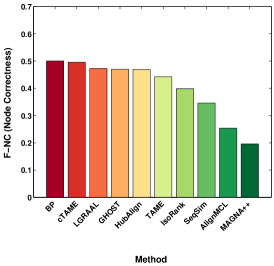
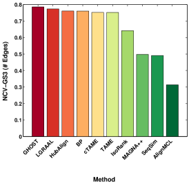
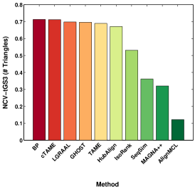
We align each pair of networks (a total of ten) separately using the different alignment methods. In Figure 1, we summarize various measures for the alignment quality of different methods when applied to the NAPAbench dataset. Figure 1(a) shows the F-score of the node correctness, which is a measure of true alignment accuracy for each method. Sparse aligners, namely BP and cTAME, have similar performance, which is better than the rest of the methods. L-GRAAL, GHOST, and HubAlign also have similar performance, which is marginally worse than sparse aligners and better than TAME. This effect can be explained by noting that true orthologs in NAPAbench, by construction, have nonzero sequence similarities. As such, these scores are highly informative for the true alignments and limiting the search space to the subset of pairs with known sequence similarity significantly simplifies the problem. TAME is primarily driven by topology and only uses sequence similarities directly in the post-processing step. Figure 1(b) and Figure 1(c) show measures of edge and triangle conservation under alignment. Results of conserved triangles is highly congruent with the actual node correctness, to a higher degree than edge conservation. To quantitatively measure this agreement, we computed the Kendall’s tau (a nonparametric rank correlation) and its corresponding p-value between the ordering of node correctness scores and edge/triangle conservation. We observed a correlation of 0.6 (p-val=$0.02$) and 0.91 (p-val=$2.98\times 10^{-5}$) between F-NC and NCV-GS3/NCV-tGS3, respectively. This suggests that both of these measures are positively related to the node correctness; however, between the two measures, triangle conservation is more significantly associated.

5.5 Alignment of human versus yeast interactomes

To assess the performance of different alignment methods when applied to real networks, we ran experiments on the yeast and human interactomes. Recall that we cannot compute node correctness in this case, since true orthologs are unknown. Therefore, we use F-score of GO function prediction as a proxy.

Figure 2: Total amount of time taken by each alignment method

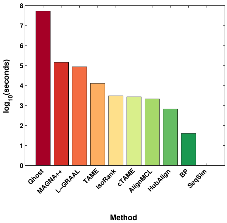
Various methods differ greatly in terms of total execution time. Figure 2 presents the running time of different methods when aligning yeast and human interactomes, reported as $log_{10}$ of the number of seconds for each method. For SeqSim method, it took less than a second to run, which we rounded up to 1s, the log of which is zero. At the other end of the spectrum, GHOST took 611 days of computational time on a single CPU to finish (we executed GHOST using 32 cores in parallel).

(a) F-score of GO function prediction

(b) GS3 (# edges)

(c) tGS3 (# triangles)

Figure 3: Comparison of alignment quality on yeast versus human dataset.

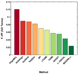
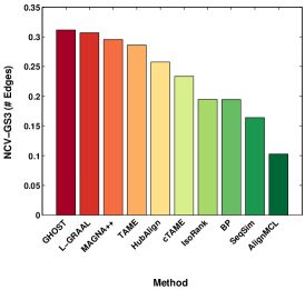
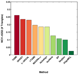
In terms of alignment quality, Figure 3 summarizes various measures computed for each alignment method. Figure 3(a) shows biological quality of the results, whereas Figures 3(b) and 3(c) illustrate edge and triangle conservation, respectively. Unlike NAPAbench, we observe a considerable difference between topological quality of alignments and their F-PF scores. Our results, similar to Malod-Dognin et al. [38], suggests that topological quality of alignments, both in terms of edges and triangles, negatively impacts the biological quality of alignments, measured as the prediction power for GO annotations. From biological point of view, we observed that AlignMCL, which is a local aligner, has the highest agreement with the GO annotations. This is consistent with the observation of Meng et al. [59] reporting that local aligners generally outperform global aligners in their prediction power for GO annotations. On the other hand, four methods with the best topological quality, namely TAME, GHOST, L-GRAAL, and MAGNA++, had the lowest F-score for predicting GO terms. In terms of edges, three methods that specifically optimize for conserved edges (GHOST, L-GRAAL, and MAGNA++) rank higher than TAME. On the other hand, in terms of triangles, TAME ranks the highest, followed by GHOST and L-GRAAL. It is notable here that the difference between the top-ranked method and runner up, in terms of edges, is $8.3\%(\frac{24,961-23,043}{23,043})$, whereas in case of triangles it is $18.6\%(\frac{76,403-64,433}{64,433})$. Moreover, note that NCV-GS3 and NCV-tGS3 are not monotonic in the number of edges/triangles. For example MAGNA++ has 14,596 conserved edges while TAME has 20,569. However, MAGNA++ has higher NCV-GS3 score.

Given the negative impact of edge/triangle conservation on the F-PF scores, we aim to find which one of them is more detrimental to the quality of GO predictions. To this end, we compute the Kendall correlation between F-PF and NCV-GS3 and NCV-tGS3, individually. Both of the correlations are negative, confirming their negative impact. However, edge conservation scores are significantly negatively correlated with F-PF (p-val = $1.6\times 10^{-2}$), whereas the negative correlation of triangle conservation scores (NCV-tGS3) and F-PF is not significant (p-val = $7.2\times 10^{-2}$), at the significance threshold of 0.05. This suggests that methods that have higher number of conserved edges impact F-PF more negatively than methods that have higher number of triangles.

To further investigate whether these results are due to the nature of GO annotations, such as heavy bias towards gene pairs with high sequence similarity, or due to the lack of biological signal, we propose a new biological measure. The main idea behind this measure is that proteins that have physical interaction are more likely to be functionally related. On the other hand, functionally related proteins are more likely to be similarly expressed in different contexts, such as different tissues/cell-types. We hypothesize that conserved edges are enriched with edges that are members of similar pathways/protein complexes and have lower false positive rate than the original network. Thus, distribution of co-expression scores between all gene pairs should have lower median than co-expression of interacting gene pairs, which in turn should have lower median than conserved edges under alignment. Using this hypothesis, we claim that a method recovers better alignment if conserved edges in the human interactome exhibit more significant difference from the background distribution of all edges.

Figure 4: Distribution of co-expression of gene pairs. Computed p-value measure the significance of the median co-expression of conserved edges being larger than the background distribution of all physical edges in the human interactome

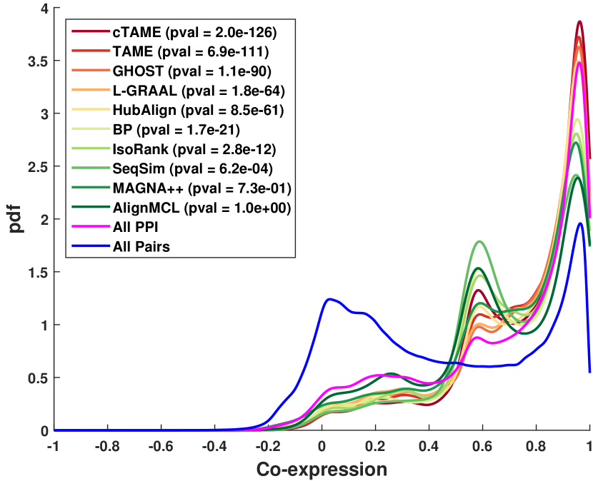
Figure 4 shows the distribution of co-expression values among different subsets of gene pairs in human interactome. First, we observe that the median of co-expression distribution for all gene pairs ($0.42$) is much smaller than the distribution for incident gene pairs on the physical edges ($0.78$). Next, we note that the left tail of co-expression distribution is heavier when considering all edges compared to only the subset of edges that are conserved in different methods. For the subset of conserved edges, there are two main peaks in the distribution, one around 0.6 and the other around 0.9. We measured the significance of change in median between the background distribution of all edges and the subset of conserved edges in each method using the Wilcoxon rank sum test. Except AlignMCL and MAGNA++, all other methods show significant shift of median to the right (p-value cutoff=0.05). All of these methods redistribute the heavy tail of PPI co-expression density to the peak of 0.6. However, among these methods, only cTAME, TAME, GHOST, L-GRAAL and HubAlign have denser (compared to the background) peaks around 0.9. cTAME and TAME show the most significant shift in the median among all other methods, with medians $0.84$ and $0.82$, respectively. This suggests that the observed inconsistency between F-PF measure and GS3/tGS3 measures is not due to the lack of biological signal, but is attributed to the nature of GO terms.

5.6 Behavior of TAME’s iterations

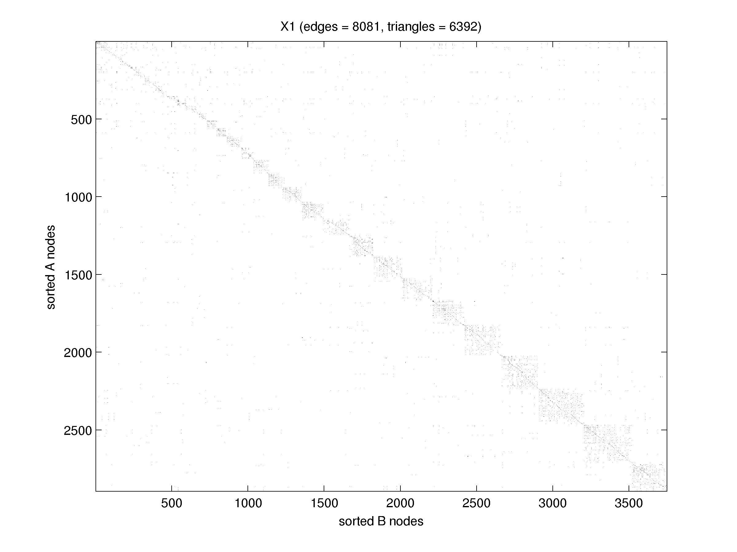
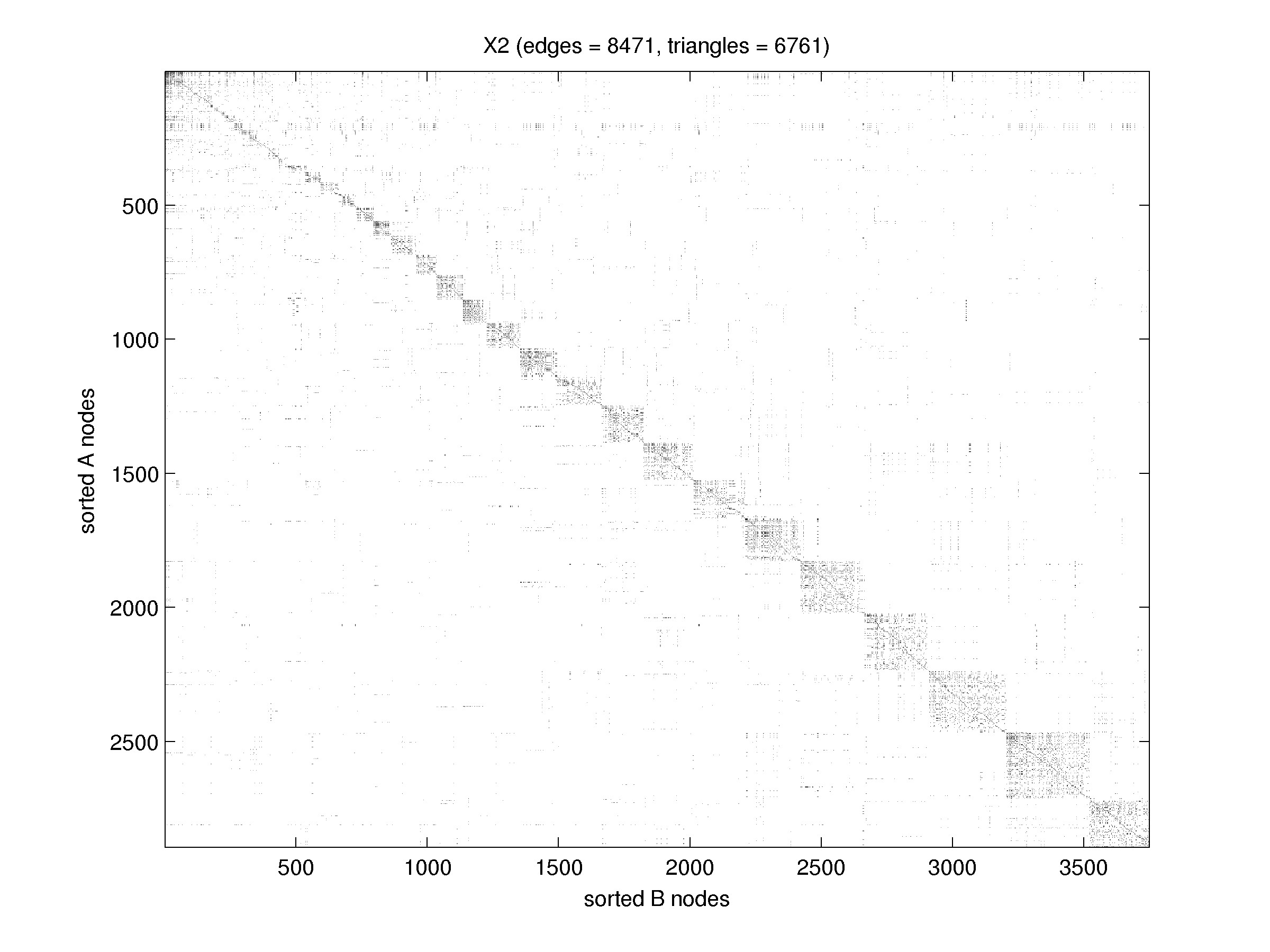
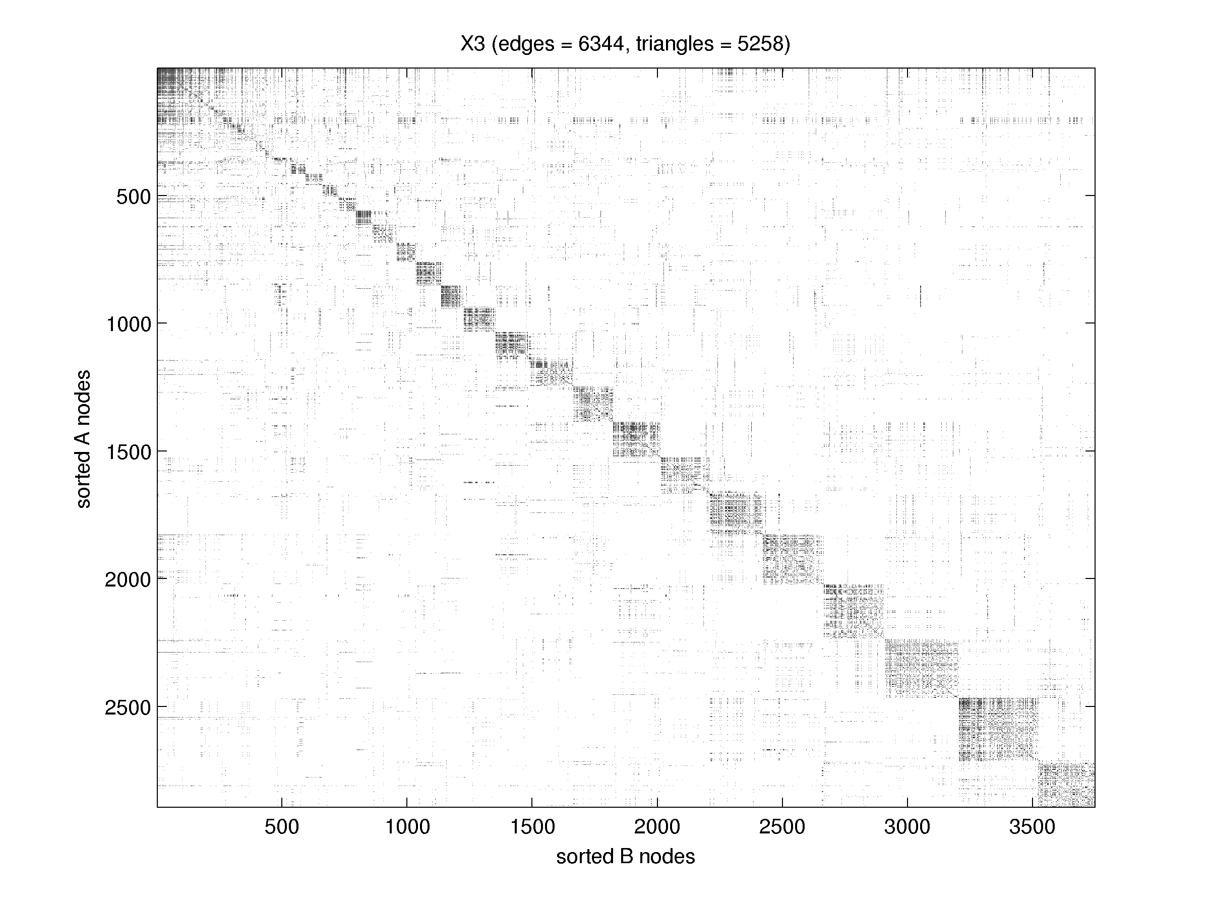
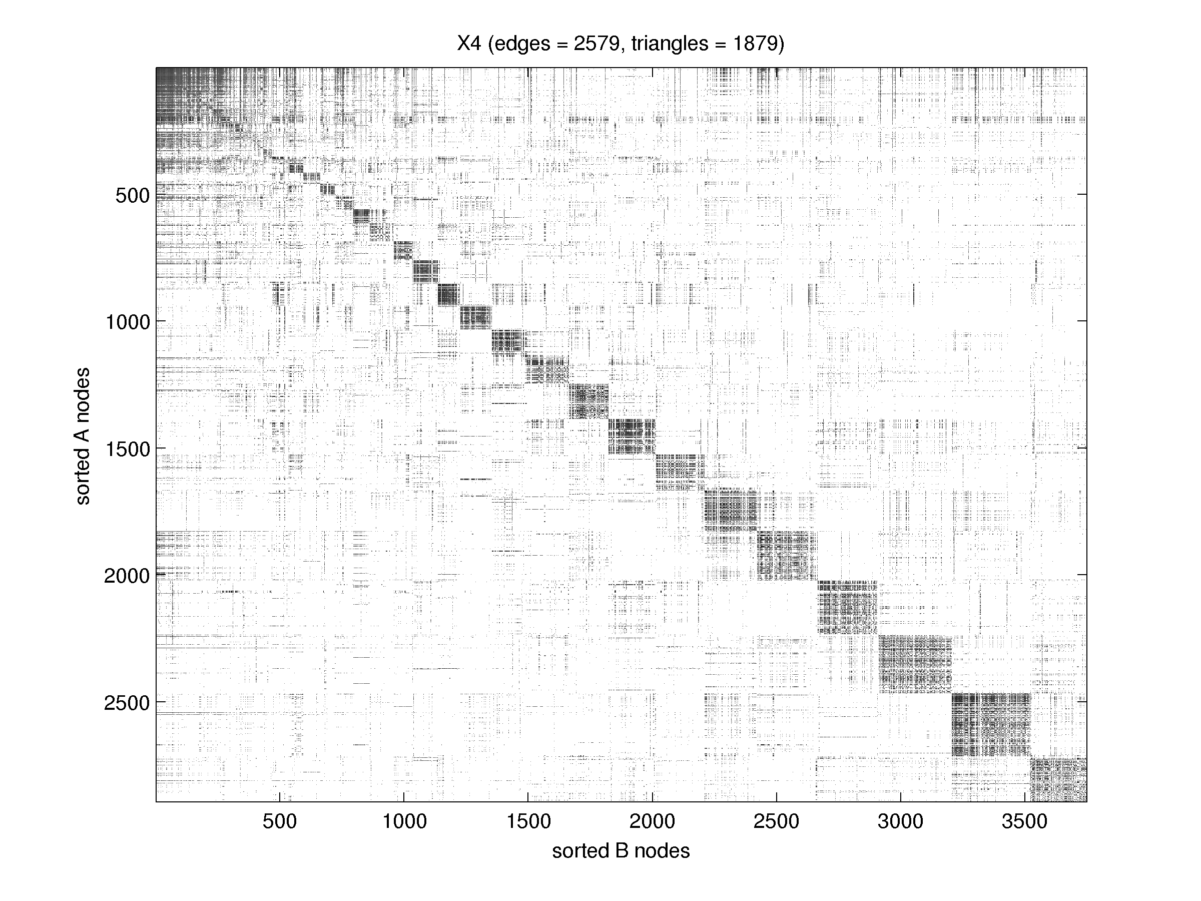
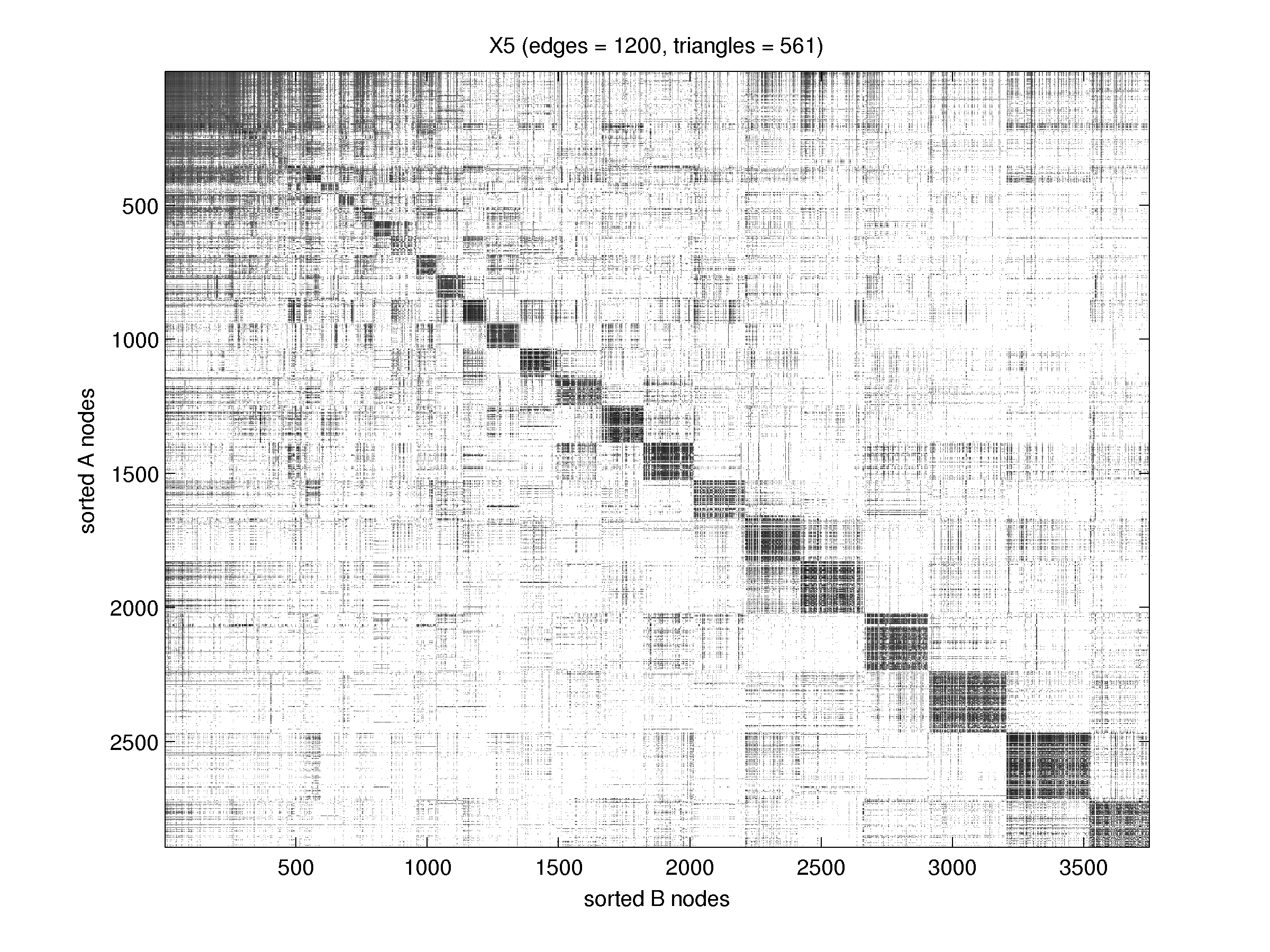
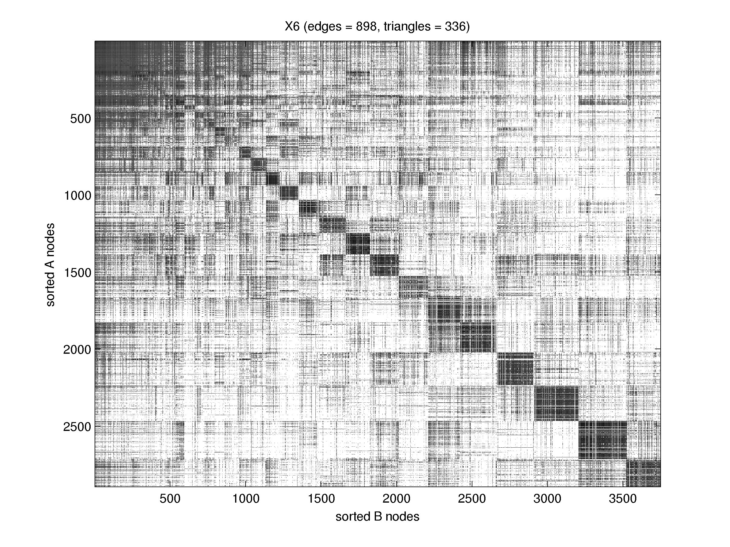
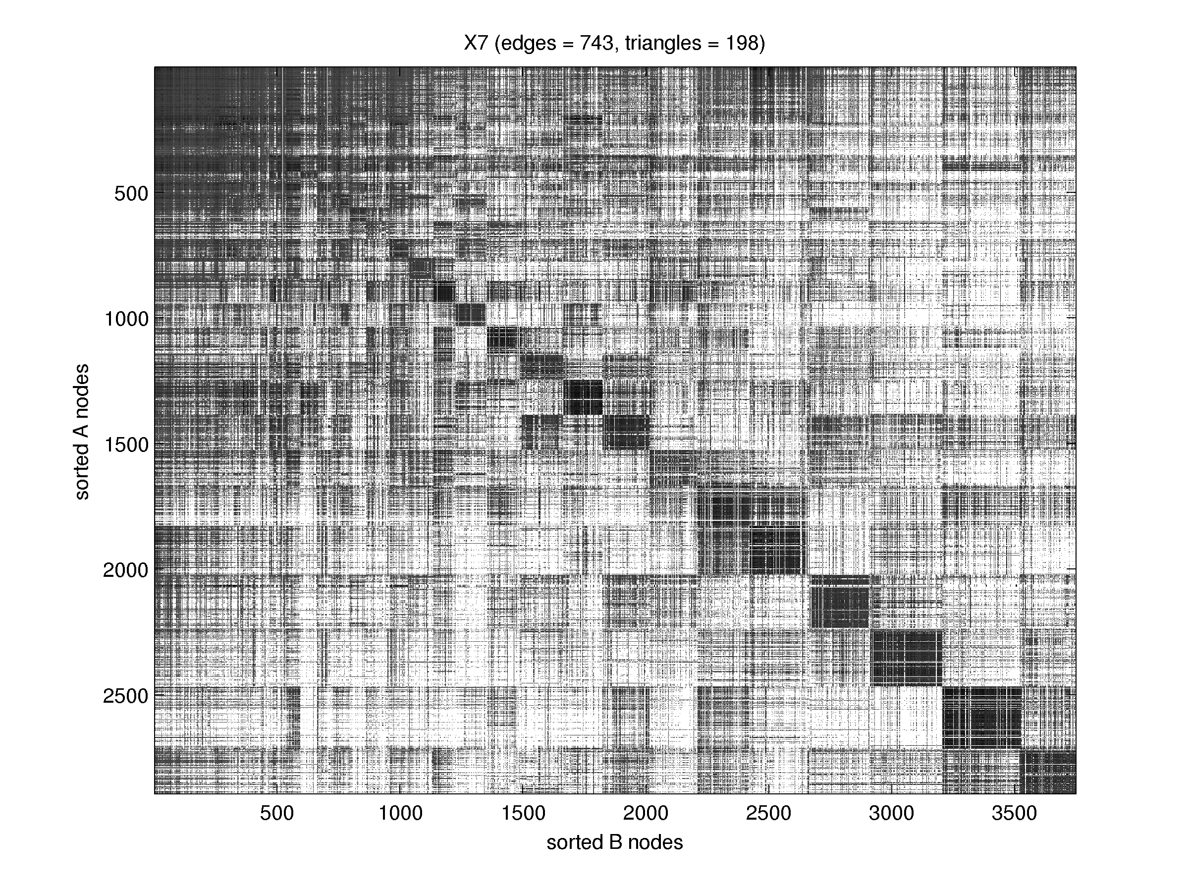
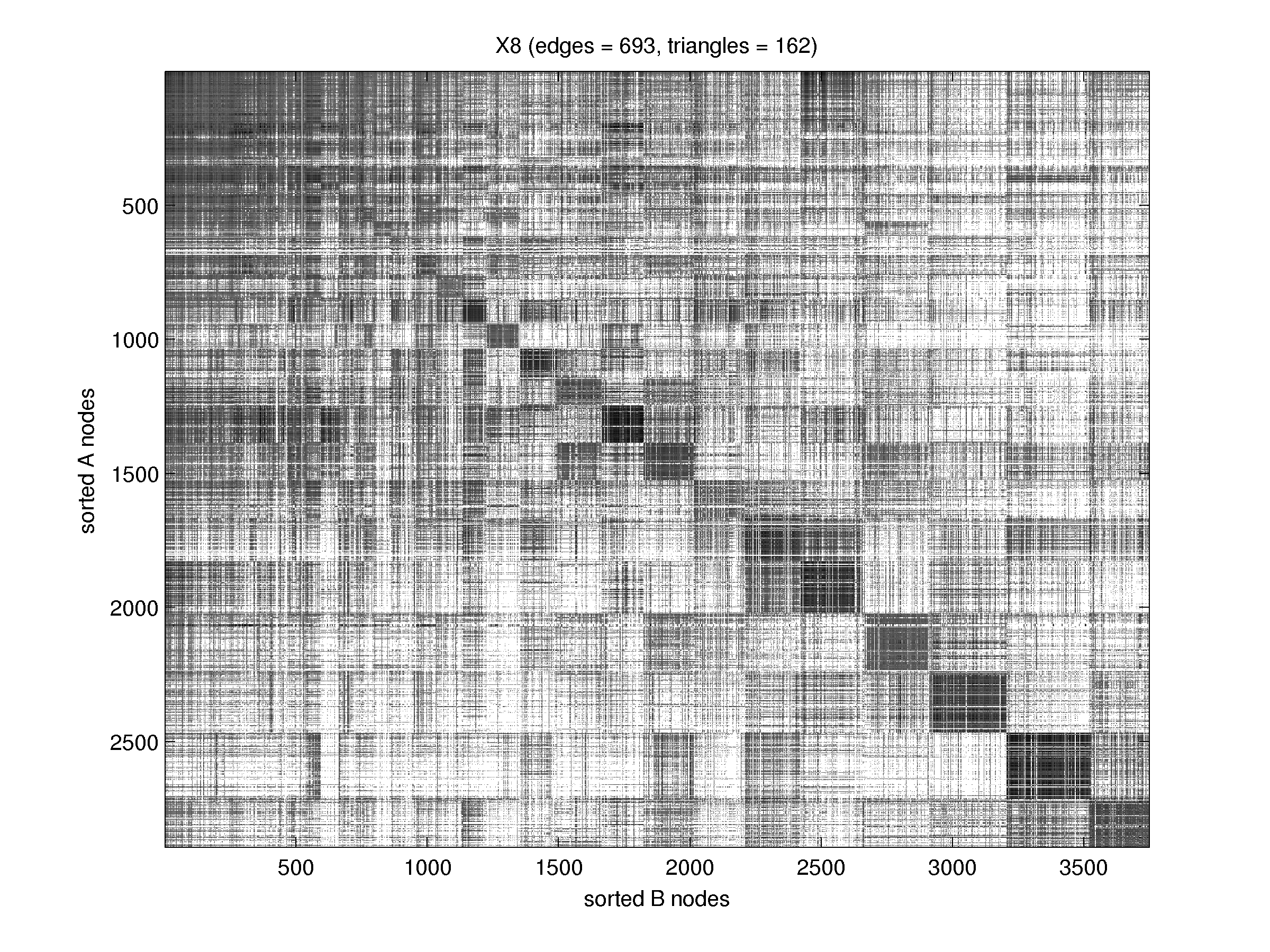
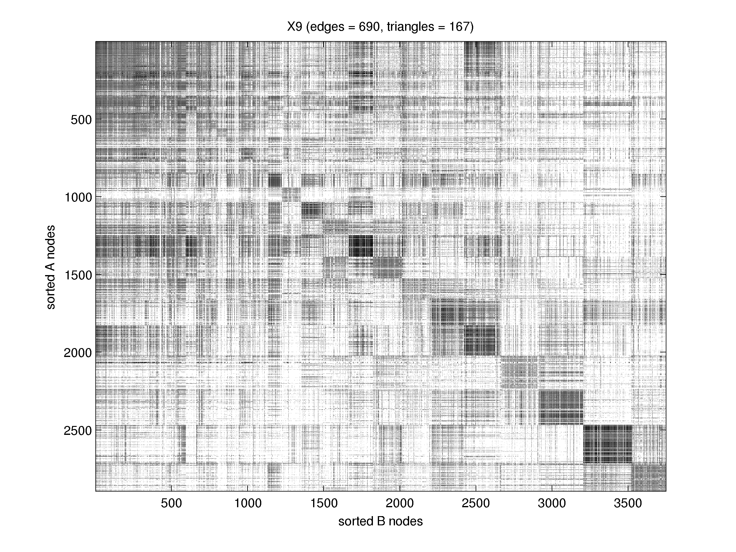
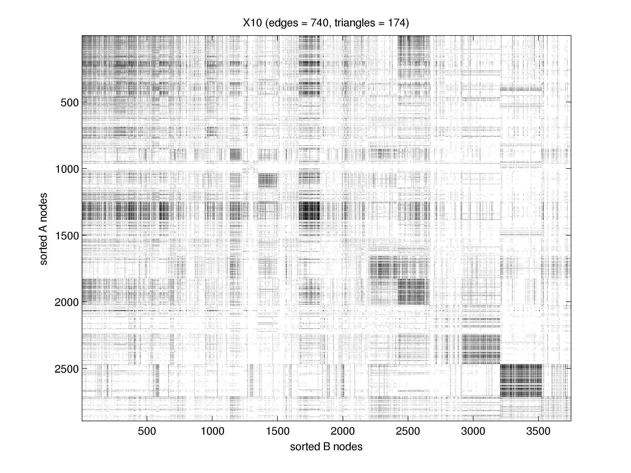
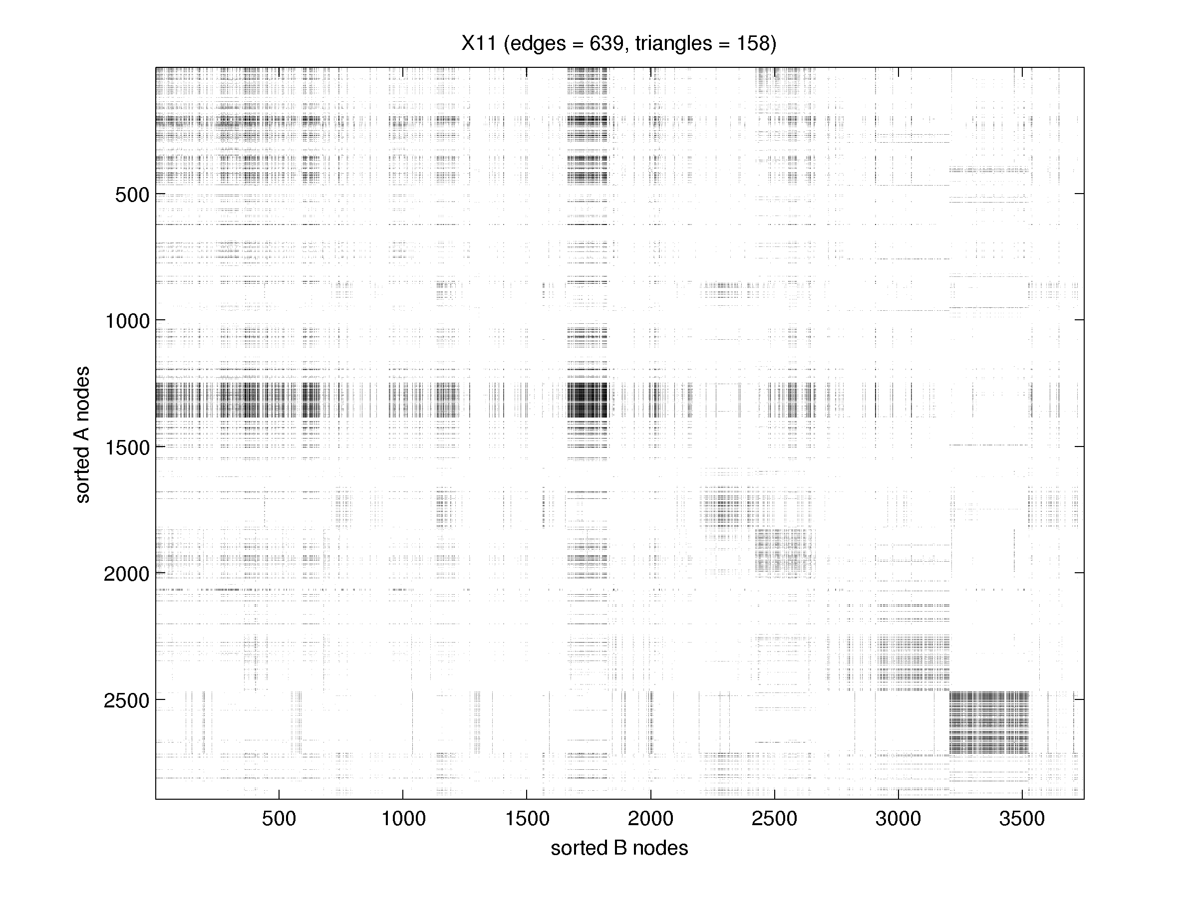
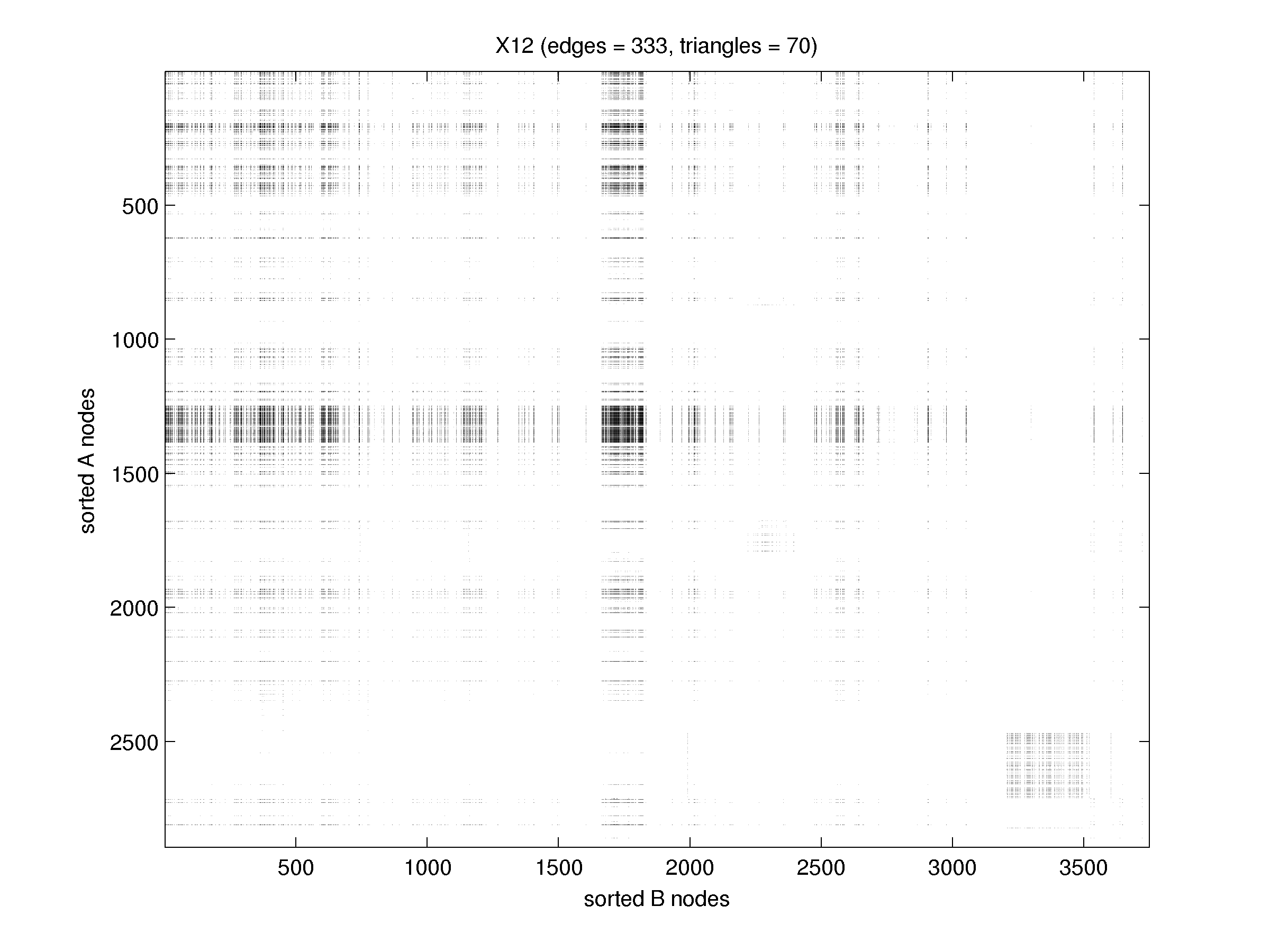
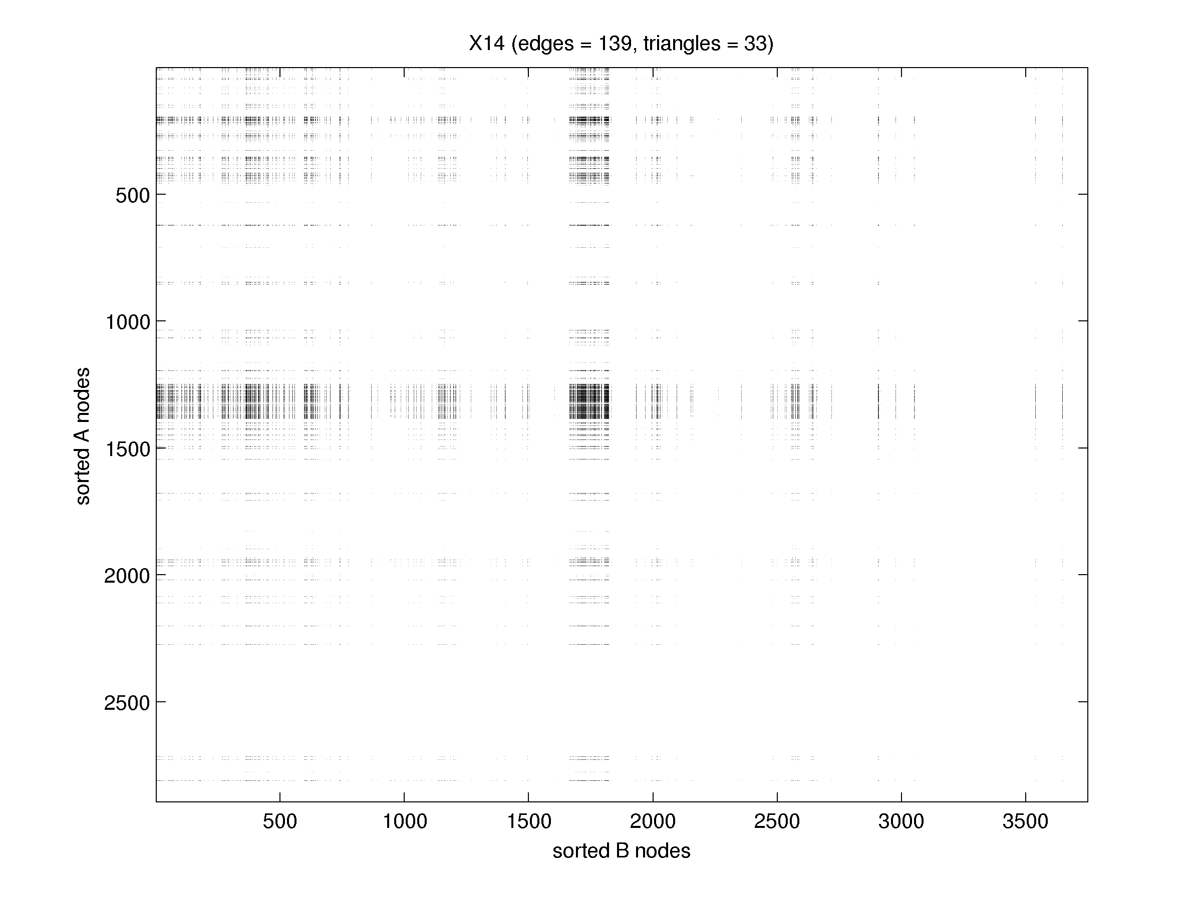
A notable aspect of TAME’s performance is that in almost all cases, the best solution occurred within the first few iterations (2-3 in all cases we tried). The same characteristic is observed both for aligning the NAPAbench and real PPI networks. We note that since SS-HOPM does not have any means to internally avoid many-to-many mappings, the dominant eigenvector of $\mathbf{\mathcal{T}}$ has a unique structure in which every node in one graph points to the most promising nodes in the other graph. In order to visualize this characteristic, we ran TAME over the Family 1 dataset in NAPAbench and visualized the structure of similarity matrix in each iteration. Figure 5 illustrates the first 15 iterations of the algorithm. We permuted rows and columns to highlight the orthologies as the diagonal of the matrix. As such, the iterations start with all sequence similarities scattered around diagonal elements (Iteration 1), and many false positive off-diagonal pairs. As iterations continue, we start by finding a block diagonal structure (Iterations 2-5), representing triangle enriched regions in the networks. As the process continues, one of the blocks emerges as the stationary point (Iterations 6-11). Subsequent iterations localize around a solution induced by this block (Iterations 12-15). We are currently seeking theoretical characterizations of this behavior that may suggest improved methods. For instance, it would be useful to avoid the transition to only one block that occurs during Iterations 6-11.

(a) Iteration 1

(b) Iteration 2

(c) Iteration 3

(d) Iteration 4

(e) Iteration 5

(f) Iteration 6

(g) Iteration 7

(h) Iteration 8

(i) Iteration 9

(j) Iteration 10

(k) Iteration 11

(l) Iteration 12

(m) Iteration 13

(n) Iteration 14

(o) Iteration 15

Figure 5: The first 15 iterations of TAME applied to Family_1 in the NAPAbench illustrated as a matrix plot of iterates $\boldsymbol{x}$ reshaped to a $\mathbf{X}$ where the true orthologs lie on the diagonal. These illustrate how the best alignments result from the information in the first few (2-5) iterations.

6 Concluding remarks and future work

In this paper, we propose an alternative formulation of the network alignment problem that uses higher-order substructures to drive the alignment process. We provide the necessary mathematical and algorithmic machinery for encoding different motifs using tensors; and, as a proof of concept, use triangle motifs to show how the framework can be applied to the network alignment problem. We show that our method outperforms state of the art techniques in terms of the total number of triangles aligned (Figures  1(c) and  3(c)), and identifies novel biological insights (Figure 4).

Our method returns a set of topological scores that can be combined with many of the other ideas in the network alignment literature. For instance, the information contained in the TAME iterates is largely orthogonal to the information produced by methods such as GHOST. We believe it is likely that these different similarity scores can be integrated – perhaps by local features of the graph topology to characterize their reliability – potentially yielding a result that is better than either.

Our ongoing work is focused on optimizing the implicit kernel, enhancing mixing properties of sequence and topological similarities, extending the main iteration to simultaneous subspace iteration with nonnegative orthogonalization, combining motifs of different sizes into the optimization problem, and understanding the theoretical basis of the success of the early iterations.

Shahin Mohammadi received his Master’s degree in Computer Science from Purdue University in December 2012 and is currently a Ph.D. candidate at Purdue. His research interests includes computational biology, machine learning, and parallel computing. His current work spans different areas of Bioinformatics/ Systems Biology and aims to develop computational methods coupled with statistical models for computationally-intensive problems.

David F. Gleich is an assistant professor of Computer Science at Purdue University. His research is on matrix computations, network and graph algorithms, and parallel and distributed computing. He received a Bachelor of Science degree from Harvey Mudd College, and a Ph.D. from Stanford University. He has been awarded a Microsoft Research Graduate fellowship, the John von Neumann postdoctoral fellowship, and an NSF CAREER award.

Tamara G. Kolda is a Distinguished Member of Technical Staff at Sandia National Laboratories in Livermore, California. Her research interests include multilinear algebra and tensor decompositions, graph models and algorithms, data mining, optimization, nonlinear solvers, parallel computing, and the design of scientific software. She received a Ph.D. from the University of Maryland. She is a fellow of the Society for Industrial and Applied Mathematics (SIAM).

Ananth Grama received a Ph.D. degree from the University of Minnesota in 1996. He is currently a Professor of Computer Sciences and Associate Director of the Center for Science of Information at Purdue University. His research interests span areas of parallel and distributed computing architectures, algorithms, and applications. On these topics, he has authored several papers and texts. He is a member of the American Association for Advancement of Sciences.

References

- [1] R. Milo et al. “Network motifs: simple building blocks of complex networks.” In Science 298.5594, 2002, pp. 824–827
- [2] N. Kashtan et al. “Efficient sampling algorithm for estimating sub-graph concentrations and detecting network motifs” In Bioinformatics 20, 2004, pp. 1746–1758
- [3] V. Batagelj and A. Mrvar “Pajek-analysis and visualization of large networks” In Springer-Verlag 2265, 2003, pp. 77–103
- [4] F. Schreiber and H. Schwöbbermeyer “Mavisto: a tool for the exploration of network motifs” In Bioinformatics 21, 2005, pp. 3572–3574
- [5] S. Wernicke and F. Rasche “FANMOD: a tool for fast network motif detection” In Bioinformatics 22, 2006, pp. 1152–1153
- [6] Zahra Razaghi Moghadam Kashani et al. “Kavosh: a new algorithm for finding network motifs.” In BMC bioinformatics 10.318, 2009 DOI: 10.1186/1471-2105-10-318
- [7] S. Mangan and U. Alon “Structure and function of the feed-forward loop network motif” In Proceedings of the National Academy of Sciences 100.21, 2003, pp. 11980–11985 DOI: 10.1073/pnas.2133841100
- [8] Shai S Shen-Orr, Ron Milo, Shmoolik Mangan and Uri Alon “Network motifs in the transcriptional regulation network of Escherichia coli.” In Nature genetics 31.1, 2002, pp. 64–68 DOI: 10.1038/ng881
- [9] Sun Sook Chung et al. “Bridging topological and functional information in protein interaction networks by short loops profiling” In Scientific Reports 5, 2015, pp. 8540 DOI: 10.1038/srep08540
- [10] Albert-László Barabási and Zoltán N. Oltvai “Network biology: understanding the cell’s functional organization” In Nature Reviews Genetics 5.2, 2004, pp. 101–113 DOI: 10.1038/nrg1272
- [11] S Wuchty, Z N Oltvai and A-L Barabási “Evolutionary conservation of motif constituents in the yeast protein interaction network” In Nature Genetics 35.2, 2003, pp. 176–179 DOI: 10.1038/ng1242
- [12] L. H. Hartwell, J. J. Hopfield, S. Leibler and A. W. Murray “From molecular to modular cell biology” In Nature 402.6761 Suppl, 1999
- [13] Tamara G. Kolda and Jackson R. Mayo “Shifted Power Method for Computing Tensor Eigenpairs” In SIAM J. Matrix Analysis Applications 32.4, 2011, pp. 1095–1124
- [14] Ondřej Šváb “Exploiting patterns in Ontology Mapping” In Proceedings of the 6th International Semantic Web Conference and 2nd Asian Semantic Web Conference (ISWC/ASWC2007), Busan, South Korea 4825, LNCS Berlin, Heidelberg: Springer Verlag, 2007, pp. 950–954 URL: http://iswc2007.semanticweb.org/papers/950.pdf
- [15] M. Chertok and Y. Keller “Efficient High Order Matching” In Pattern Analysis and Machine Intelligence, IEEE Transactions on, 2010, pp. 2205–2215 DOI: 10.1109/TPAMI.2010.51
- [16] Sayed Mohammad Ebrahim Sahraeian and Byung-Jun Yoon “A Network Synthesis Model for Generating Protein Interaction Network Families” In PLoS ONE 7, 2012, pp. e41474 DOI: 10.1371/journal.pone.0041474
- [17] R B Kelley and el. “Conserved pathways within bacteria and yeast as revealed by global protein network alignment” In PNAS 100(20), 2003
- [18] Brian P. Kelley et al. “PathBLAST: a tool for alignment of protein interaction networks” In Nucleic Acids Research 32.Web-Server-Issue, 2004, pp. 83–88
- [19] Roded Sharan et al. “Identification of Protein Complexes by Comparative Analysis of Yeast and Bacterial Protein Interaction Data” In Journal of Computational Biology 12.6, 2005, pp. 835–846
- [20] Roded Sharan et al. “Conserved patterns of protein interaction in multiple species.” In Proceedings of the National Academy of Sciences of the United States of America 102.6, 2005, pp. 1974–1979
- [21] J Flannick et al. “Graemlin: general and robust alignment of multiple large interaction networks” In Genome Research 16.9, 2006, pp. 1169–1181
- [22] Jason Flannick et al. “Automatic Parameter Learning for Multiple Network Alignment” In RECOMB, 2008, pp. 214–231
- [23] Mehmet Koyutürk, Ananth Grama and Wojciech Szpankowski “Pairwise Local Alignment of Protein Interaction Networks Guided by Models of Evolution” In RECOMB, 2005, pp. 48–65
- [24] M. Koyutürk et al. “Pairwise Alignment of Protein Interaction Networks” In Journal of Computational Biology 13(2), 2006, pp. 182–199
- [25] Marco Mina and Pietro Hiram Guzzi “Improving the Robustness of Local Network Alignment: Design and Extensive Assessment of a Markov Clustering-Based Approach.” In IEEE/ACM transactions on computational biology and bioinformatics / IEEE, ACM 11.3, 2014, pp. 561–72 DOI: 10.1109/TCBB.2014.2318707
- [26] Rohit Singh, Jinbo Xu and Bonnie Berger “Pairwise Global Alignment of Protein Interaction Networks by Matching Neighborhood Topology” In Proceedings of the 11th Annual International Conference on Research in Computational Molecular Biology, RECOMB’07 Oakland, CA, USA: Springer-Verlag, 2007, pp. 16–31 URL: http://dl.acm.org/citation.cfm?id=1758222.1758224
- [27] R. Singh, J. Xu and B. Berger “Global alignment of multiple protein interaction networks with application to functional orthology detection” In PNAS 105.35, 2008, pp. 12763–12768
- [28] Chung-Shou Liao et al. “IsoRankN: spectral methods for global alignment of multiple protein networks” In Bioinformatics 25.12 Oxford, UK: Oxford University Press, 2009, pp. i253–i258
- [29] Giorgos Kollias, Shahin Mohammadi and Ananth Grama “Network Similarity Decomposition (NSD): A Fast and Scalable Approach to Network Alignment” In IEEE Transactions on Knowledge and Data Engineering 24.12, 2011, pp. 2232–2243 DOI: 10.1109/TKDE.2011.174
- [30] Giorgos Kollias, Madan Sathe, Shahin Mohammadi and Ananth Grama “A fast approach to global alignment of protein-protein interaction networks.” In BMC research notes 6.1, 2013, pp. 35 DOI: 10.1186/1756-0500-6-35
- [31] Oleksii Kuchaiev et al. “Topological network alignment uncovers biological function and phylogeny.” In Journal of the Royal Society, Interface / the Royal Society 7.50, 2010, pp. 1341–54 DOI: 10.1098/rsif.2010.0063
- [32] T Milenković, W L Ng, W Hayes and N Przulj “Optimal network alignment with graphlet degree vectors” In Cancer Inform 9, 2010
- [33] Oleksii Kuchaiev and Natasa Przulj “Integrative network alignment reveals large regions of global network similarity in yeast and human.” In Bioinformatics (Oxford, England) 27.10, 2011, pp. 1390–6 DOI: 10.1093/bioinformatics/btr127
- [34] Vesna Memišević and Nataša Pržulj “C-GRAAL: common-neighbors-based global GRAph ALignment of biological networks” In Integrative biology : quantitative biosciences from nano to macro 4.7, 2012, pp. 734–43 DOI: 10.1039/c2ib00140c
- [35] Gunnar Klau “A new graph-based method for pairwise global network alignment” In BMC Bioinformatics 10.Suppl 1, 2009, pp. S59 DOI: 10.1186/1471-2105-10-S1-S59
- [36] Mohammed El-Kebir, Jaap Heringa and Gunnar W. Klau “Lagrangian Relaxation Applied to Sparse Global Network Alignment” In CoRR abs/1108.4358, 2011 URL: http://dblp.uni-trier.de/db/journals/corr/corr1108.html#abs-1108-4358
- [37] Mohsen Bayati, David F Gleich, Amin Saberi and Ying Wang “Message-Passing Algorithms for Sparse Network Alignment” In ACM Trans. Knowl. Discov. Data 7.1 New York, NY, USA: ACM, 2013, pp. 3:1–3:31 DOI: 10.1145/2435209.2435212
- [38] Noël Malod-Dognin and Nataša Pržulj “L-GRAAL: Lagrangian graphlet-based network aligner.” In Bioinformatics (Oxford, England) 31.13, 2015, pp. 2182–9 DOI: 10.1093/bioinformatics/btv130
- [39] Rob Patro and Carl Kingsford “Global network alignment using multiscale spectral signatures.” In Bioinformatics (Oxford, England) 28.23, 2012, pp. 3105–14 DOI: 10.1093/bioinformatics/bts592
- [40] Leonid Chindelevitch, Cheng-Yu Ma, Chung-Shou Liao and Bonnie Berger “Optimizing a global alignment of protein interaction networks.” In Bioinformatics (Oxford, England) 29.21, 2013, pp. 2765–73 DOI: 10.1093/bioinformatics/btt486
- [41] Vikram Saraph and Tijana Milenković “MAGNA: Maximizing Accuracy in Global Network Alignment.” In Bioinformatics (Oxford, England) 30.20, 2014, pp. 2931–40 DOI: 10.1093/bioinformatics/btu409
- [42] V Vijayan, V Saraph and T Milenković “MAGNA++: Maximizing Accuracy in Global Network Alignment via both node and edge conservation.” In Bioinformatics (Oxford, England) 31.14, 2015, pp. 2409–11 DOI: 10.1093/bioinformatics/btv161
- [43] Maoguo Gong, Zhenglin Peng, Lijia Ma and Jiaxiang Huang “Global Biological Network Alignment by Using Efficient Memetic Algorithm.” In IEEE/ACM transactions on computational biology and bioinformatics / IEEE, ACM, 2015 DOI: 10.1109/TCBB.2015.2511741
- [44] Somaye Hashemifar and Jinbo Xu “HubAlign: an accurate and efficient method for global alignment of protein-protein interaction networks.” In Bioinformatics (Oxford, England) 30.17, 2014, pp. i438–44 DOI: 10.1093/bioinformatics/btu450
- [45] M. Koyuturk et al. “Pairwise Alignment of Protein Interaction Networks” In Journal of Computational Biology 13(2), 2006, pp. 182–199
- [46] Shahin Mohammadi and Ananth Grama “Biological Network Alignment” In Functional Coherence of Molecular Networks in Bioinformatics Springer, 2011, pp. 97–136 URL: http://www.springerlink.com/content/t18030hh8x02w635/fulltext.pdf
- [47] Connor Clark and Jugal Kalita “A comparison of algorithms for the pairwise alignment of biological networks.” In Bioinformatics (Oxford, England) 30.16, 2014, pp. 2351–2359 DOI: 10.1093/bioinformatics/btu307
- [48] Ahed Elmsallati, Connor Clark and Jugal Kalita “Global Alignment of Protein-Protein Interaction Networks: A Survey.” In IEEE/ACM transactions on computational biology and bioinformatics / IEEE, ACM, 2015 DOI: 10.1109/TCBB.2015.2474391
- [49] L.-H. Lim “Singular Values and Eigenvalues of Tensors: A Variational Approach” In CAMSAP’05: Proceeding of the IEEE International Workshop on Computational Advances in Multi-Sensor Adaptive Processing, 2005, pp. 129–132
- [50] Mohsen Bayati, David F Gleich, Amin Saberi and Ying Wang “Message-Passing Algorithms for Sparse Network Alignment” In ACM Trans. Knowl. Discov. Data 7.1 New York, NY, USA: ACM, 2013, pp. 3:1–3:31 DOI: 10.1145/2435209.2435212
- [51] Robert Preis “Linear Time 1/2 -approximation Algorithm for Maximum Weighted Matching in General Graphs” In Proceedings of the 16th Annual Conference on Theoretical Aspects of Computer Science, STACS’99 Trier, Germany: Springer-Verlag, 1999, pp. 259–269 URL: http://dl.acm.org/citation.cfm?id=1764891.1764924
- [52] Arif Khan et al. “Efficient approximation algorithms for weighted b-Matching.” In SIAM Journal on Scientific Computing, 2016 (to appear)
- [53] Wan Kyu Kim and Edward M. Marcotte “Age-Dependent Evolution of the Yeast Protein Interaction Network Suggests a Limited Role of Gene Duplication and Divergence” In PLoS Computational Biology 4.11, 2008, pp. e1000232 DOI: 10.1371/journal.pcbi.1000232
- [54] John C Wootton and Scott Federhen “Statistics of local complexity in amino acid sequences and sequence databases” In Computers & Chemistry 17.2, 1993, pp. 149–163 DOI: 10.1016/0097-8485(93)85006-x
- [55] W R Pearson and D J Lipman “Improved tools for biological sequence analysis” In Proc. Natl. Acad. Sci. 85, 1988, pp. 2444–2448+
- [56] T F Smith and M S Waterman “Identification of common molecular subsequences.” In Journal of molecular biology 147.1, 1981, pp. 195–7 URL: http://www.ncbi.nlm.nih.gov/pubmed/7265238
- [57] K. G. Ardlie et al. “The Genotype-Tissue Expression (GTEx) pilot analysis: Multitissue gene regulation in humans” In Science 348.6235, 2015, pp. 648–660 DOI: 10.1126/science.1262110
- [58] Stephen R Piccolo et al. “Multiplatform single-sample estimates of transcriptional activation.” In Proceedings of the National Academy of Sciences of the United States of America 110.44, 2013, pp. 17778–83 DOI: 10.1073/pnas.1305823110
- [59] Lei Meng, Aaron Striegel and Tijana Milenkovic “Local versus Global Biological Network Alignment”, 2015 arXiv: http://arxiv.org/abs/1509.08524
- [60] M Ashburner et al. “Gene ontology: tool for the unification of biology. The Gene Ontology Consortium.” In Nature genetics 25.1, 2000, pp. 25–9 DOI: 10.1038/75556
- [61] Tamara G. Kolda and Jackson R. Mayo “An Adaptive Shifted Power Method for Computing Generalized Tensor Eigenpairs” In SIAM Journal on Matrix Analysis and Applications 35.4, 2014, pp. 1563–1581 DOI: 10.1137/140951758
![[Uncaptioned image]](/html/1510.06482/assets/figures/shahin-photo.png) |