Recovery from Giant Eruptions in Very Massive Stars
Abstract
We use a hydro-and-radiative-transfer code to explore the behavior of a very massive star (VMS) after a giant eruption – i.e., following a supernova impostor event. Beginning with reasonable models for evolved VMSs with masses of and , we simulate the change of state caused by a giant eruption via two methods that explicitly conserve total energy: 1. Synthetically removing outer layers of mass of a few while reducing the energy of the inner layers. 2. Synthetically transferring energy from the core to the outer layers, an operation that automatically causes mass ejection. Our focus is on the aftermath, not the poorly-understood eruption itself. Then, using a radiation-hydrodynamic code in 1D with realistic opacities and convection, the interior disequilibrium state is followed for about 200 years. Typically the star develops a wind with a mass loss rate that begins around and gradually decreases. This outflow is driven by -mechanism radial pulsations. The 1D models have regular pulsations but 3D models will probably be more chaotic. In some cases a plateau in the mass-loss rate may persist about 200 years, while other cases are more like Car which lost and then had an abnormal mass loss rate for more than a century after its eruption. In our model, the post-eruption outflow carried more mass than the initial eruption. These simulations constitute a useful preliminary reconnaissance for 3D models which will be far more difficult.
Subject headings:
stars: evolution — stars: mass loss — stars: winds, outflows — stars: variables: general — hydrodynamics — methods: numerical1. Introduction
Very massive stars (VMSs) with spend substantial fractions of their short lifetimes close to the Eddington limit. After leaving the main sequence, they stay in the blue part of the HR diagram, left of the HD limit (Humphreys & Davidson, 1979). It is known from the excess of nitrogen in their ejecta that these stars have gone far into core hydrogen-burning via the CNO bi-cycle. As the star lost most of its hydrogen in winds, and helium was dredged-up from the core, the outer layers are helium rich. This is confirmed by observations of Car (Davidson et al. 1986; Dufour et al. 1997). Being so close to the Eddington limit, VMSs are susceptible to instabilities and disturbances, both internally and from companion stars, which can undermine the delicate balance between radiation pressure and gravity. Perhaps the most exotic effect that can happen to such a fragile structure is a Giant Eruption, in which the VMS loses – of its mass (e.g., Humphreys & Davidson 1994; Smith & Owocki 2006; Van Dyk & Matheson 2012).
These eruptions are sometimes called “Supernova Impostors”, and in some cases it is unclear whether the VMS underwent a giant eruption, or actually exploded as a supernova. Some terminal explosions of VMSs are associated with type IIn SNe (e.g., Gal-Yam et al. 2007; Kochanek et al. 2012), but other types have also been suggested, such as the so-called type IIb, an event which transitions from type II to Ib (Groh et al. 2013).
In that context it is interesting to mention SN 2011ht, a peculiar Type IIn supernova with significant ”impostor” characteristics in its spectrum (Humphreys et al. 2012; Roming et al. 2012). An example with a more complex history is SN 2009ip. In 2009 it experienced a giant eruption initially labeled a SN event; but then a series of later outbursts arose in 2011–2012, leaving researchers uncertain about whether the terminal event had finally occurred or not (Drake et al. 2012; Fraser et al. 2013; Kashi et al. 2013; Mauerhan et al. 2013, 2014; Margutti et al. 2014; Pastorello et al. 2013; Prieto et al. 2013; Soker & Kashi 2013; Tsebrenko & Soker 2013; Graham et al. 2014).
Since this topic has not received much theoretical attention, far less is known about the impostors and giant eruptions than about true supernovae. The energy budget may allow either a core event or an instability in the outer layers, or conceivably even both. Only a few examples have been observed for sufficient lengths of time, the most famous case being Car’s Great Eruption in the nineteenth century. Some conjectural models suggest interior mechanisms (e.g., Stothers & Chin 1997; Guzik et al. 1997; Dwarkadas & Balick 1998; Langer et al. 1999; Baraffe et al. 2001; Shaviv 2001; González et al. 2004,2010; Woosley et al. 2007; Chatzopoulos & Wheeler 2012; Shacham & Shaviv 2012; Smith et al. 2011; Smith 2013), while others employ tidal intervention by companion stars (Cassinelli 1999; Kashi & Soker 2010; Kashi 2010). The phenomenon may be physically related to LBV eruptions which are much smaller. Using a nonlinear pulsation gas dynamics code, Guzik & Lovekin (2014) found that the Eddington limit can be crossed repeatedly in the pulsation driving region of the stellar envelope, very likely generating mass loss. The evolution of a massive star depends on its metallicity, rotation, and mass-loss history as well as initial mass (e.g, Heger et al. 2005); and a nearby companion can alter the composition and angular momentum distribution – maybe triggering an outburst.
A VMS can lose 1% to 20% of its mass in one or more giant eruptions (e.g., Humphreys & Davidson 1994; Langer 2012; Davidson & Humphreys 2012a) leaving it in a state of thermal and rotational disequilibrium. Davidson (2012) commented on possible time scales for the subsequent recovery. For example, a change of state in the mass-loss rate is currently observed in Car (Davidson et al. 2005; Mehner et al. 2012, 2014), suggesting that the recovery time is in the order of centuries, and the trend has been remarkably unsteady (Humphreys et al., 2008).
The relevant timescale for the recovery is unclear. A thermal timescale depends on which layers are included, and we note that Car’s current luminosity amounts to ergs (half the amount released in the Great Eruption) in about 200 years. However, the transport rate may have been faster soon after the event because thermal disequilibrium was worse then. Angular momentum, chemical composition, and perhaps even entropy can be transported by turbulent viscosity, whose timescale in Car may be as short as 25 years (Davidson, 2012). The important point is that recovery timescales may be anywhere in the range 10 to 300 years, based only on simplified reasoning without detailed simulations. As Car, SN2009ip and other objects have shown, it may well be that during this recovery another giant eruption takes place.
In a previous experiment of giant eruption and recovery of an evolved star, Harpaz & Soker (2009) took an evolved star model (after hydrogen in the core was depleted) and modeled its response to a very high mass loss. Their model had a convective core, then a radiative zone, followed by another convective shell and another outer radiative zone with very little mass. It developed a steep entropy rise above the convective core. To simulate an eruption, they subtracted mass from the evolved star at a constant rate of for a duration of 20 years, after which they reduced the mass-loss rate and traced the star for additional 200 years. Their code, as they note, cannot conserve energy when removing the mass from the star. In a response to the mass loss the star contracted (mainly due to the removal of the outer high entropy layers) and released a huge amount of gravitational energy that caused its luminosity to increase to values up to almost . Harpaz and Soker suggest that this will lead to a runaway mass loss.
In this paper we report on several experiments to model the recovery of a VMS from a Giant eruption. The star is modeled from the core to the surface including the wind using the radiation transfer-hydro code FLASH. This involves 12 or more orders of magnitude in density, and requires simulations with a high level of refinement. As a first step, to test our physical model and input parameters we describe the results of one-dimentional simulations which include the entire star and its wind. They provide an initial view and guidance for 3D simulations.
Car will appear often in the following text, merely because it is the only post-eruption VMS that has been observed well. Its luminosity, ejected mass, post-eruption wind and photometric record, etc., are known far better than any other supernova impostor (Humphreys & Martin 2012; Davidson 2012, and many references therein). Car’s Great Eruption in 1830–1860 may have been triggered by the companion star near periastron (Kashi & Soker 2010 and references therein), but that possibility has little effect on the subsequent internal physics. This paper concerns post-eruption VMS’s in general, not specifically Car.
In principle we cannot be certain of Car’s evolutionary state, because the surface wind does not directly represent the core structure. The observed surface helium abundance shows that it is somewhat evolved. The timescale for late stages is very short, and one might expect hydrogen should then be scarce. Therefore the simplest as well as more probable choice is that it has not yet reached the helium burning stage – but there is no known way to prove this. These questions obviously require further investigation. The mass loss has been unsteady, and for more than a century it was too strong to be explained by line driving (Davidson 2012).
2. Methods
2.1. Obtaining a Pre-Eruption Model
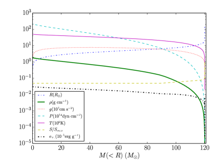
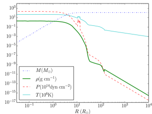
Our moderately evolved non-rotating VMS has , , and its radius would correspond to if there were no opaque wind. In order to obtain a consistent internal structure, we begin with a ZAMS star and evolve it with the 1D MESA code (Paxton et al. 2011,2013,2015). In order to obtain a post main sequence helium abundance , suggested by the Car example, much of the hydrogen-rich envelope must be ejected. Since the conventional mass-loss prescriptions usually employed with MESA (e.g., De Jager, Vink, etc.) cannot achieve this, we adopt the following simple behavior. (1) Initially the star evolves away from the ZAMS with a mass loss rate of . (2) When falls below (the bi-stability jump), the rate increases to . Obviously this is somewhat arbitrary, but the same is true for all published VMS evolution models, since their mass-loss behavior at that stage is very poorly understood. The purpose of our MESA usage is merely to obtain a “reasonable” internal structure just before the VMS eruption. Since a very high mass-loss rate tends to increase , the above procedure creates a negative feedback that “locks” the star at . At the time when its mass has fallen to , the luminosity is and the radius is about . The helium fraction at the surface is then . Helium burning has not begun yet, and it is burning hydrogen via the CNO bi-cycle. This model is adequate for our numerical experiment, and is credible in the sense that it resembles the best-observed eruptive VMS, Car. Its structural properties are shown in Fig. 1.

2.2. Simulating the results of an Eruption
The next stage is to simulate a giant eruption in the VMS. The basic instability is not yet understood (indeed there may be more than one mechanism), and our goal is not to model it but rather to explore the aftermath. The only unquestionable facts are that a substantial mass is ejected along with to ergs of energy, and that total energy must be conserved. Fortunately the energy requirement is only a small fraction of the star’s total thermal energy. We use two operationally different approaches. (1) Synthetically removing mass in a timescale much shorter than the relevant thermal timescale. In other words, we suddenly truncate the star’s mass distribution. Energy to unbind and lift the ejecta is artificially extracted from mass layers that are not removed. If the removal timescale is longer than a few weeks, most of the star remains fairly close to hydrostatic equilibrium. The main unknown is the radial distribution of the special energy-supply fund, which depends on the nature of the instability. In any case the outermost surviving layers have far less energy than the deeper layers; so, after a short-lived redistribution process, the behavior depends only moderately on the assumed distribution. In the models described here, we simply assume that the thermal energy decreases by a constant fraction per unit mass.
(2) Extracting thermal energy from the core. In this approach we artificially move some thermal energy from the inner region to the outer layers, without explicitly removing any mass. The location where we deposit the energy is the radius which has the same gravitational binding energy above, so the energy is sufficient to free the layers above. The resulting structure is far out of thermal equilibrium, and automatically ejects some mass. Thermal energy is extracted from mass layers as done for method 1. Hydrostatic equilibrium is not preserved at the beginning.
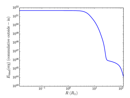
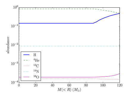
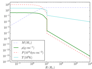
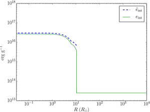
In one experiment we used method 1 and removed (5% of the star’s mass), adjusting the energy parameters so that the ejecta had a terminal speed of . This speed is the escape velocity (not corrected for radiation pressure) of the star at the location where the energy is deposited. The ejected part initially had a gravitational binding energy ergs. The remaining nearly-hydrostatic object had a radius of only about 10.5 , and the first panel in Fig. 2 shows its properties after the simulated eruption.
Outside the stellar radius we added a fictitious extension with negligible mass and energy, for practical reasons noted in section 2.3. The second panel in Fig. 2 shows a similar model using method 2. The quantitative details may be expressed in different ways, but the basic nature of the star in Fig. 2 resembles a post-eruption VMS in almost any orthodox scenario.
2.3. The Hydrodynamic Simulation
We now come to the main topic: the recovery of a VMS after a giant eruption. After manipulating the stellar model, we import the data into the hydrodynamic code FLASH (Fryxell et al., 2000). We use version 4.2.2 of the FLASH code. It employs an Eulerian grid with adaptive mesh refinement (AMR). We used a 1D spherical grid with reflecting boundary conditions at the center and ‘diode’ boundary conditions at the outer boundary, such that gas can flow out to the guard cells but not back into the grid. This allows mass loss from the star by the stellar wind. We used Rosseland-mean opacity data from OPAL (Iglesias & Rogers, 1996). As the nuclear timescale is much longer than the duration of the simulation, nuclear reactions are turned off in our simulation.
The stellar model was imported into FLASH with a low-density extension out to . This fictitious envelope merely provided space for the star to expand in the Eulerian grid. It had , with negligible mass and energy. These details had practically no effect, as that region rapidly filled with much denser material from the star.
A convection algorithm for 1D simulations, such as mixing length theory, is not incorporated. In order to simulate convection in 1D in FLASH, we used a simplified prescription where was limited to the adiabatic value, . This does not provide an estimate of the convective energy flux, but that quantity becomes important for our results only in the outer regions where radiative flux dominates (section 3 below).
We let the star run for a few hundred years to trace its evolution. The stability of the code was tested with a polytrope, and also with our VMS model with no mass removal. In both cases the star remained in hydrostatic equilibrium and no mass was lost.
3. Results.
| Run | Method 1 | Star Mass | Mass initially removed/ | Energy shifted/ | 3,4 | Total Mass lost |
| () | equivalent energy shifted 2 () | removed () | () | () | ||
| 1 | (1) | 120 | 6 | 10.5 | 33 | |
| 2 | (1) | 120 | 3 | 12.3 | 6.5 | |
| 3 | (1) | 120 | 9 | 9.50 | 34 | |
| 4 | (2) | 120 | 6 | 11 | ||
| 5 | (2) | 120 | 3 | 6 | ||
| 6 | (2) | 120 | 9 | 13 | ||
| 7 | (2) | 80 | 2 | 3.5 | ||
| 8 | (2) | 80 | 4 | 6 | ||
| 9 | (2) | 80 | 6 | 9 | ||
| 10 | (2) | 80 | 8 | 14.5 |
1 See text for details.
2 In method 2 we shift energy from the core to outer layers. This column list the mass that this energy is able to unbind from the star. Other sources of energy remove additional mass.
3 For method 1, all layers initially outside radius were removed in the first step of the experiment, see text.
4 Initial radii of the and stars were and , respectively. Their central temperatures were and , respectively.
We examine the stellar properties of the different runs at various times from the beginning of the eruption experiment (). starting with run 1. Fig. 3 shows the properties of the star as a function of time: stellar radius, effective temperature, luminosity, mass, Eddington ratio, mass-loss rate and convective mass-loss rate.
An observationally important question is how to define the “apparent radius” in a super-Eddington wind. Fig. 5, for example, shows the exterior optical depth in run 1 at various times. The radius where , often quoted for photospheres, is very large and cool: and . In fact has no physical significance in a convex opaque wind, where most emergent photons come from . Moreover, scattering dominates the opacity in cases of interest here. Hence the characteristic temperature of escaping continuum radiation represents the thermalization depth, where (e.g., Hubeny & Mihalas 2014; Davidson 1987). In our models this occurs near , which we adopt to define the star’s apparent or observable radius . We find that even though the star expands to after the eruption, its effective temperature stays above , on the blue side of the HD limit on the HR diagram.
Another question is how to define the luminosity when the star is far from equilibrium. Fig. 6 shows the radiative luminosity , maximum convective luminosity , and the total luminosity , at different times for runs 1 and 4 (discussed below). The local luminosity depends on because the star is not in thermal equilibrium. The radiative luminosity is calculated using the diffusion approximation
| (1) |
where is the radius, is the temperature, is the opacity, and is the radiation constant. At large radii, when approaching the stellar surface, and in the wind, the estimate of based on the diffusion approximation in eq. (1) becomes invalid. The reason is that the because of the low density, the mean free path of photons becomes comparable with, and finally larger than, the remaining travel distance to the stellar surface. This results in a large overestimate of . We therefore plot it only up to . The region at a few shows strong decline in . We will return to this detail later.
Only a maximum convective luminosity can be calculated here:
| (2) |
where is the local speed of sound. The true value is presumably smaller. Fig. 6 shows that the luminosity at is dominated by radiation. The Eddington ratio is calculated using the Thomson scattering opacity because the absorption fraction is small.
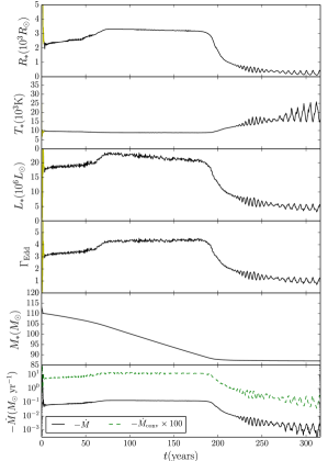
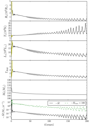
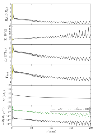
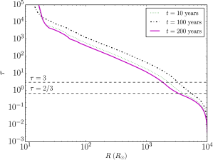
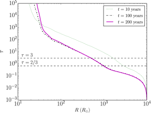
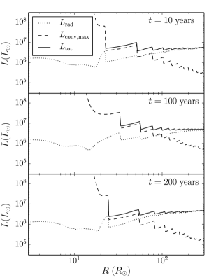
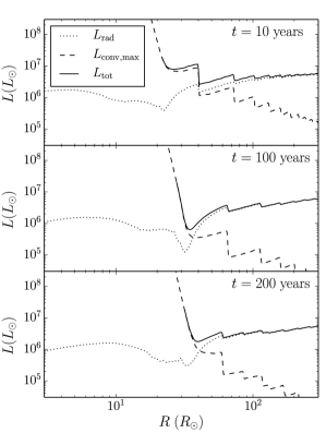
Table 1 shows the mass-loss results for ten calculative runs. The time dependence of run 1, for example, is portrayed in Fig. 3. This model continued to eject material at a high rate long after the initial event, and ultimately lost more than three times as much mass as the amount that we artificially removed to initiate the process. For several years the star approached a sort of quasi-equilibrium and expanded into our coordinate grid, and then, during the interval , it had a mass-loss rate of the order of . This qualitatively resembles the case of Car, but was more extreme and more protracted. There are strong hints that Car had a rate a century ago (Humphreys et al., 2008), and by the year 2000 this had declined to roughly (Davidson & Humphreys 1997; Hillier et al. 2001). Thus a model intermediate between our runs 1 and 2 would somewhat resemble Car’s history in the past 160 years. As explained below, the underlying cause for mass-loss both in that stage and later is a -mechanism induced pulsation. As declined in run 1 after yr, most of the quantities in Fig. 3 showed obvious outward-moving waves.
VMSs have regions with strong convection. In the outer layers of the star, where convection becomes inefficient due to decline in (where is the speed of sound), the radiative Eddington factor
| (3) |
(where is the radiative luminosity, and ) becomes larger than 1. The radius where this occurs is called the critical radius , and the density at this location is the critical density . If we put the sonic radius for a wind outflow at this location we can derive a convective mass-loss rate
| (4) |
The sixth row on the left panel of Fig. 3 shows for run 1 together with the actual mass-loss rate. It can be seen that the actual mass-loss rate is very close to the convective mass-loss rate.
The reason for the decrease in mass-loss rate at later times is that as mass is lost the profile of the star changes, and layers with steeper density gradient are exposed. These layers have a higher gravitational binding energy, and therefore are more difficult to remove.
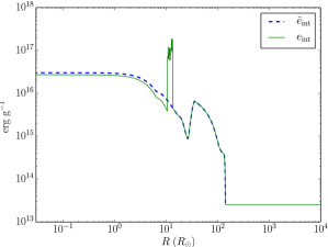
In Fig. 7 we show the properties of the star as a function of radius (including the extension), for different times after the eruption. Note the following phases:
-
1.
At early times the original low density - low pressure extension still exists. It can be seen as a very inconspicuous feature at in the line representing in upper panel of the Fig. 7. It takes the density profile (of the star and its wind) to expand to the edge of the grid. As mentioned, we experimented with different extensions, and found that the original extension profile does not affect the results, if the mass in the extension is much smaller then the stellar mass.
-
2.
The core of the star was initially compressed as a result of the eruption. After it returned to its original density.
-
3.
After the star develops a structure that conserves its shape as time goes by. The profiles do change as a result of an ongoing mass-loss, but the general shape remains roughly the same.
The behavior of the star at might not be very meaningful as it depends on the details of the method we use. That being said, for the two methods we tried we do however get similar results for that initial time after the eruption.
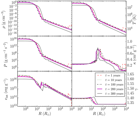
By examining the regions of high opacity, we can interpret the decrease in mass loss after yr. The strong opacity peak is identified as the “Iron Bump”, located at . Before yr the location of the peak is in relatively low density region, such that the pulsations that are strongest at that region, can push the gas outwards and result in the high mass loss. As mass is depleted from the star, its structure changes. As it approaches yr, the opacity peak location coincides with the high slope of the density towards the inner layers of the star. These layers are more massive and cannot be easily pushed out by the pulsations. The energy of the pulsations still travels out, removing the low density outer layers of the star. Gradually over a few decades, the density in the outer layers becomes smaller, and the mass-loss rate decreases. As the density decreases so is the optical depth, therefore the location of by which we determine the radius moves inwards. During that time the lower density in outer layers causes the density profile of the star to expand, such that the density gradient becomes smaller, and the density in the center decreases.
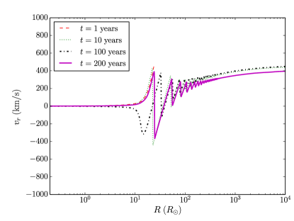
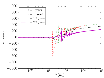
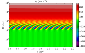
The left panel of Fig. 8 shows the radial velocity profiles for run 1 (left panel), and run 4 (right panel) Ripples in the velocity profile (and also in the pressure profile – see third panel of Fig. 7) started developing. Each layer expands into low density and pressure, and then the following layer expands into a denser region and with a higher pressure, and so on. The exact shape of the ripples is a result of the stellar density and pressure profile. In a 3D model, presumably the ripples shown in our figures become much less coherent when averaged over latitude and longitude – i.e., waves propagate in various directions with random elements not present in our radial 1D calculations. The cumulative effect, however, would be an outward mass and energy flow.
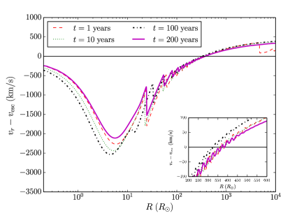
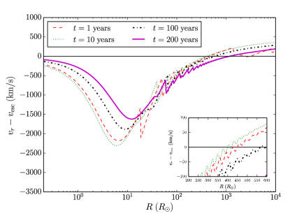
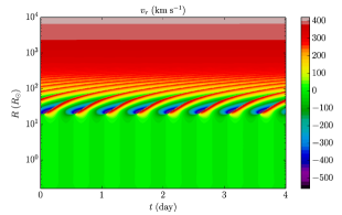
At later times a more or less similar velocity profile is observed, with the velocity at the outer edge of the grid . This is comparable to the terminal velocities observed in VMSs. The velocity profile has a region where the velocity fluctuates between positive (outward) and negative (inward) values, as can be seen in Fig. 8. This is the region where we found pulsations (see below). Further out the star develops a wind that causes it to lose mass. Fig. 9 shows the radial velocity after subtracting the escape velocity. This is the radius where the gas escapes from the star.
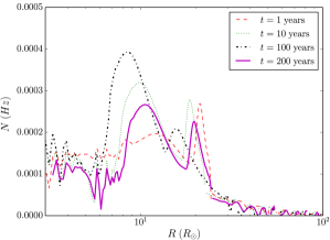
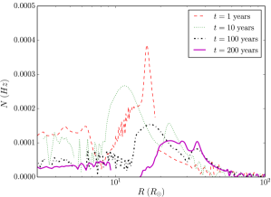
We calculate the Brunt-Väisälä frequency of the star (the frequency for adiabatic pulsations)
| (5) |
as a function of radius, for different times (Fig. 10), where is the gravitational acceleration and is the adiabatic index. There is a strong peak in the same layers where the pulsation occurs. As time moves on, the peak moves slightly outwards, indicating that the strong pulsation layer is propagating as mass is lost from the star and the density becomes smaller.
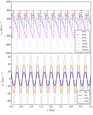
We analyze the pulsation by restarting run 1 at , and running it with higher sampling. In order to know the required sampling rate, to avoid any aliasing, we take the maximum Brunt-Väisälä frequency at , , which corresponds to hours. The Nyquist sampling rate (maximum allowed sampling rate) to avoid aliasing is therefore hours. We restart the run with high sampling rate and let it run for . We then slice the star into layers and plot the radial velocity of each layer as a function of time, as shown in Fig. 11 and Fig. 12. Note that positive velocities indicate flow in the positive radial direction. We can identify a number of radial regions:
-
1.
The internal part of the star from the center up to is almost not pulsating at all and has a radial velocity close to .
-
2.
At a transition begins into strong radial pulsations, with amplitudes increasing up to a peak at . It is also seen that at different radii the pulsations have a phase difference. The phase difference is gradually increasing with radius.
-
3.
After there is a transition region where there are variations in the radial velocity as a function of time, but not periodic pulsations.
-
4.
At the pulsations almost completely stop, and the wind has only a radius dependent velocity profile, with an acceleration trend.
We do not predict observable rapid pulsations, since the amplitude goes to close to zero at the surface of the star, and since the waves can become non radial and incoherent in three dimensions.
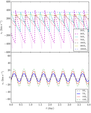
As mentioned above, the region of the star at a few shows strong decline in . As shown in Fig. 12, this is the same regions where stellar pulsation is strongest. In this region pulsation transforms energy carried by photons to kinetic energy, generating the wind.
The FLASH code has an Eulerian grid. In order to know what happens to a layer of the star as a result of the pulsation we need to follow an element of gas in its trajectory, i.e., in a Lagrangian way. We therefore start at a certain radius and check the properties at some initial time. Then, we follow the gas element that started at this radius to different radii in the star according to its velocity. Fig. 13 presents density, temperature, pressure, adiabatic index, opacity and radial velocity at starting radius , as a function of time, after , for runs 1 and 4. We also calculate the quantity , which for adiabatic pulsations should remain constant with time. We find that varies in a periodic way with the same period of the other quantities – so the pulsations are not adiabatic. This is not surprising since mass is lost from the system. An important feature we see in both panels of Fig. 13, is that when the pressure increases there is an increase in opacity. This increase in opacity acts to extract radiation energy from the inner parts of the star, essentially the -mechanism.
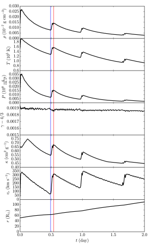
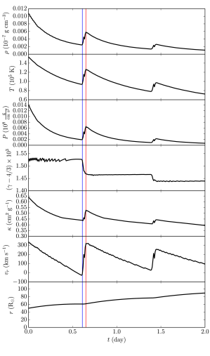
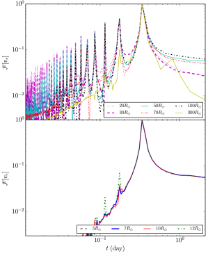
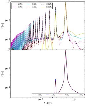
Fig. 14 shows the Fourier transform of the radial velocity as a function of time-scale, at different radii. We find a pronounced peak at . Note that there is a phase difference between the pulsations at different radii, that is not seen in the Fourier space but clearly seen in the velocity space (Figs. 11 and 12). Other modes are also seen with smaller time scales, especially for the radii where strong pulsation exists. At larger radii there is no evident pulsation time scale smaller than .
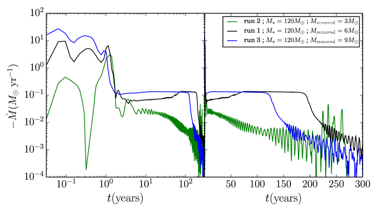
Runs 2 and 3 used method 1. The only change was the amount of mass that was removed from the star. The result are shown in Table 1. We see a different behavior between run 2 (where is removed) and runs 1 and 3 (where and are removed, respectively). Runs 1 and 3 show the same qualitative behavior: a strong mass loss followed by a long duration plateau after which there is a decline accompanied by fluctuations. Note also that run 3, even more extreme than run 1, did not result in much more total mass ejected. This is a consequence of the star’s initial structure, having a steep gravitational binary energy below the outer .
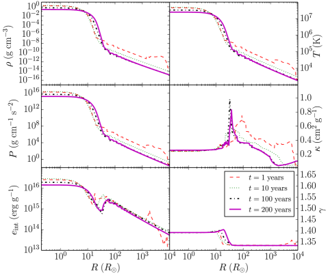
Run 4 uses the same initial stellar model, but instead of removing mass, we take the energy required to do so and extract it from the inner layers (method 2 in section 2.2). Specifically, we reduce the thermal energy of each mass element by a constant small fraction, and deposit that energy in a narrow band of outer layers. The latter region was adjusted to coincide with the deepest layers that were eventually ejected (). Its width was arbitrarily chosen to have a width of , and the energy was deposited in the those layers weighted by layer’s mass. Narrowing or widening the band of layers (up to a factor of 3) did not significantly alter the results for yr. The right panel of Fig. 2 shows the properties of the star after extracting energy from the core to a layer, according to method 2, and adding an extension. The left panels of Fig. 3 shows the properties of the star as a function of time. While the mass and its derivative are calculated unambiguously, the radius, temperature and luminosity are the estimated at . These are not actual photosphere values. The location changes rapidly as a function of time. However, this does not mean that the stellar photosphere is so variable. Most of the mass is lost in the first of the simulation. This corresponds to the eruption itself, while later times show the recovery of the star from the eruption.
The right/second panels of Figs. 3 and 5 – 14 show the results of run 4. Fig. 7 shows that in run 4 the star is dominated by radiation pressure. In the envelope, after the eruption only radiation pressure plays a role in pushing the wind; gas pressure is negligible. As seen in Fig. 6, the outer luminosity is radiative luminosity, and the convective luminosity is negligible (this is true for run 1 and all other runs studied here).
Fig. 8 and Fig. 9 show us that the wind velocities that are reached for run 4 are comparable of run 1, reaching . Run 4 has a higher shown in Fig. 5, but not by much. The Fourier analysis in Figs. 11 and 12 shows that qualitatively the pulsations for both methods are similar, though somewhat higher frequency for method 1. The difference in the frequency are not related to the different masses that the two methods have, as at the time analyzed () their masses are similar . This is despite run 1 having much lower mass at later times due to the strong runaway mass loss. In fact the frequencies only differ by a factor of up to , and considering the slightly different properties (density, temperature) such a small change is not surprising. As noted earlier, the waves in a 3D model will surely be less coherent than those in our figures, and hence more chaotic.
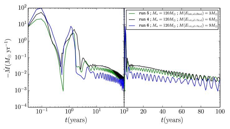
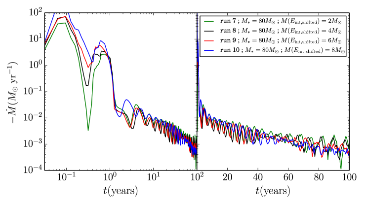
For method 2 we ran three runs for the stellar model with different energy extracted from the core, which is equivalent to the energy required for ejecting a certain amount of mass, as indicated in Table 1 (referred to as “equivalent energy shifted”). The total mass lost is larger then this amount, as other sources of energy that operate after the eruption remove the extra mass. The properties and the evolution with time of the three runs are very similar qualitatively. Fig. 16 shows a comparison of the mass-loss rate as a function of time of the three runs. Most of the mass is lost in the first of the simulation. We can clearly see a trend in the mass-loss rate during that phase, with the more energy extracted from the core the higher the mass-loss rate during that time. At later time there is no clear trend in our results.
We ran four more runs for a different stellar model with , following the same procedure used to obtain the stellar model. The four runs differ by the energy extracted from the core, which is equivalent to the energy required for ejecting a certain amount of mass, as indicated in Table 1. Fig. 17 shows a comparison of the mass-loss rate as a function of time of the four runs. The same trends seen for the stellar model are also observed here.
4. Summary and Discussion
In each model described here, a giant VMS eruption tends to prolong itself for reasons that do not depend much on the instability that started it. The later aftermath includes a very strong wind () which decays in one or two centuries. This outcome appears physically reasonable, since the initial mass-loss obviously produces a state of serious internal disequilibrium. (For example, a large amount of radiation energy suddenly finds itself less trapped than it was before.) Moreover, the picture also appears consistent with the only well-observed giant-eruption survivor, Car. The main cause for doubt is that a 2D or 3D outburst might, in principle, abate sooner; but we have not noticed any simple or obvious reasons why this should be the case, apart from factors of order 2. Recently Quataert et al. (2015) have, like us, employed 1D calculations for a related problem. Our models were planned to serve as a 1D reconnaissance of the problem, pending 2D and 3D work which will be far more difficult. In that sense, perhaps the most important result here is that 3D models now seem more promising in view of the quantitative 1D behavior.
When tracking the propagation of gas elements, there is a correlation between the compression of the gas and the increase in opacity. We therefore classify the resulting pulsations as from -mechanism. The so called “strange-mode” instability was suggested as a possible driving force for winds and even giant eruptions (e.g. Sterken et al. 1996; van Genderen et al. 1995; Cox et al. 1997; Guzik et al. 1997, 2012). Exploring the existence or absence of strange modes in the pulsations we obtained is beyond the scope of the present paper.
The amplitude of the pulsations is almost certainly exaggerated, simply because these are 1D calculations. In 3D the same instability exists but would not be radially coherent. High amplitudes may exist locally, but their directions and phases would vary with location in the envelope. Therefore the averaged mass loss rate is credible, but there is no reason to expect it have such obvious, coherent global pulsations.
To check the effects of rotation, we also ran a MESA model where the initial rotation rate is of the critical maximum. Adding rotation had little effect when studying the eruption, as the outer shells, which possess most of the angular momentum, were removed.
Our simulations do not explain the major fluctuations that Car has exhibited since its 1830–1860 Great Eruption. A second outburst was observed around 1890, a sort of change-of-state rapidly occurred around 1940–1950, and another rapid transition began in the 1990’s (Humphreys et al. 1999; Martin et al. 2006; Mehner et al. 2010; Humphreys & Martin 2012 and other references therein) – almost hinting at a 50-year quasi-periodicity. Many authors have speculated that these peculiarities have something to do with the companion star, because tidal effects may be appreciable in the primary’s wind-acceleration zone. But such effects are much weaker in the star’s interior, . It will be interesting to learn whether 3D simulations behave unsteadily.
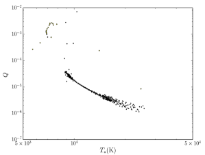
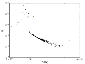
Our simulations also provide information about how the giant eruption may have looked. Davidson (1987) calculated the radiation temperature of luminous stars undergoing eruptions. He found that the temperatures do not fall much below even for enormous mass-loss rates. Davidson (1987) defined the quantity as
| (6) |
and showed that there is an asymptote close to . This is analogous to the Hayashi Limit since it results from the rapid decrease of opacity below . For run (4) we calculate the value of for different times during the simulation. Fig. 18 shows the results. The yellow diamonds are early times in the simulation and the values of are not accurate. The black dots are from times later in the simulation. We find that the simulation gives , the same results calculated analytically by Davidson 111 Rest et al. (2012) suggested that 6000 K is too high based on light-echo spectra, but they relied on comparisons with stellar atmospheres rather than opaque outflows. A wind with a photosphere can produce relatively cool spectral features, cf. Davidson & Humphreys (2012b). . After the eruption, we found the stellar temperature is above , so it stays on the blue side of the HD limit on the HR diagram.
Though 2D and 3D simulations are computationally very expensive, and will be investigated in a future paper, we have studied the same problem in 2D for a short time interval ( years). The case studied is the same as in run 4. The results we obtained are qualitatively the same. We do find an interesting result that could not be obtained in 1D simulations. Under the assumption that the source of the eruption is the core (method 2), the eruption causes a Richtmyer-Meshkov instability in the star in the first few days after the eruption (Fig. 19). This causes strong mixing of elements from the core to outer layers. It may therefore explain why the ejecta of Car is Nitrogen rich. Nuclear processed material from the core reaches the outer layers and eventually is ejected from the star.
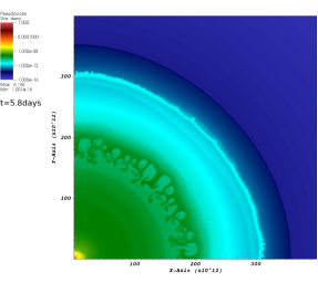
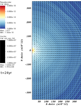
We also find in our 2D simulation that the star experiences pulsations and ejects mass. Fig. 20 shows a density map with velocity vectors taken years after the eruption. We see similar pulsations as in the 1D simulation, but as expected in the discussion above they are not as intense as in the 1D case.
Full multi-dimensional simulations will be the subject of a future paper. The tools that we are developing for studying giant eruptions will have other uses in studying other objects that experience large mass loss.
We acknowledge support provided by National Science Foundation through grant AST-1109394. This work was carried out in part using computing resources at the University of Minnesota Supercomputing Institute (MSI). This work used the Extreme Science and Engineering Discovery Environment (XSEDE), which is supported by National Science Foundation grant number ACI-1053575. We thank Alexander Heger for enlightening discussions about the simulations. We thank Joyce Guzik and Ken Chen for helpful suggestions. We thank an anonymous referee for helpful comments.
References
- Baraffe et al. (2001) Baraffe, I., Heger, A., & Woosley, S. E. 2001, ApJ, 550, 890
- Cassinelli (1999) Cassinelli, J. P. 1999, Eta Carinae at The Millennium, 179, 358
- Chatzopoulos & Wheeler (2012) Chatzopoulos, E., & Wheeler, J. C. 2012, ApJ, 760, 154
- Cox et al. (1997) Cox, A. N., Guzik, J. A., & Soukup, M. S. 1997, Luminous Blue Variables: Massive Stars in Transition, 120, 133
- Davidson (2012) Davidson, K. 2012, Astrophysics and Space Science Library, 384, 43
- Davidson (1987) Davidson, K. 1987, ApJ, 317, 760
- Davidson et al. (1986) Davidson, K., Dufour, R. J., Walborn, N. R., & Gull, T. R. 1986, ApJ, 305, 867
- Davidson et al. (2005) Davidson, K., Martin, J., Humphreys, R. M., et al. 2005, AJ, 129, 900
- Davidson & Humphreys (1997) Davidson, K., & Humphreys, R. M. 1997, ARA&A, 35, 1
- Davidson & Humphreys (2012a) Davidson, K., & Humphreys, R. M. 2012, Astrophysics and Space Science Library, 384
- Davidson & Humphreys (2012b) Davidson, K., & Humphreys, R. M. 2012, Nature, 486, 1
- Drake et al. (2012) Drake, A. J., Howerton, S., McNaught, R., et al. 2012, The Astronomer’s Telegram, 4334, 1
- Dufour et al. (1997) Dufour, R. J., Glover, T. W., Hester, J. J., et al. 1997, Luminous Blue Variables: Massive Stars in Transition, 120, 255
- Dwarkadas & Balick (1998) Dwarkadas, V. V., & Balick, B. 1998, AJ, 116, 829
- Fraser et al. (2013) Fraser, M., Inserra, C., Jerkstrand, A., et al. 2013, MNRAS, 433, 1312
- Fryxell et al. (2000) Fryxell, B., Olson, K., Ricker, P., et al. 2000, ApJS, 131, 273
- Ferguson et al. (2005) Ferguson, J. W., Alexander, D. R., Allard, F., et al. 2005, ApJ, 623, 585
- Gal-Yam et al. (2007) Gal-Yam, A., Leonard, D. C., Fox, D. B., et al. 2007, ApJ, 656, 372
- González et al. (2004) González, R. F., de Gouveia Dal Pino, E. M., Raga, A. C., & Velazquez, P. F. 2004, ApJ, 600, L59
- González et al. (2010) González, R. F., Villa, A. M., Gómez, G. C., et al. 2010, MNRAS, 402, 1141
- Graham et al. (2014) Graham, M. L., Sand, D. J., Valenti, S., et al. 2014, ApJ, 787, 163
- Groh et al. (2013) Groh, J. H., Meynet, G., & Ekström, S. 2013, A&A, 550, L7
- Guzik et al. (1997) Guzik, J. A., Cox, A. N., Despain, K. M., & Soukup, M. S. 1997, Luminous Blue Variables: Massive Stars in Transition, 120, 138
- Guzik & Lovekin (2012) Guzik, J. A., & Lovekin, C. C. 2012, The Astronomical Review, 7, 13
- Guzik & Lovekin (2014) Guzik, J. A., & Lovekin, C. C. 2014, arXiv:1402.0257
- Harpaz & Soker (2009) Harpaz, A., & Soker, N. 2009, New A, 14, 539
- Heger et al. (2005) Heger, A., Woosley, S. E., & Baraffe, I. 2005, The Fate of the Most Massive Stars, 332, 339
- Hillier et al. (2001) Hillier, D. J., Davidson, K., Ishibashi, K., & Gull, T. 2001, ApJ, 553, 837
- Hubeny & Mihalas (2014) Hubeny, I., & Mihalas, D. 2014, Theory of Stellar Atmospheres, by I. Hubeny and D. Mihalas. Princeton, NJ: Princeton University Press, 2014,
- Humphreys & Davidson (1979) Humphreys, R. M., & Davidson, K. 1979, ApJ, 232, 409
- Humphreys & Davidson (1994) Humphreys, R. M., & Davidson, K. 1994, PASP, 106, 1025
- Humphreys et al. (2008) Humphreys, R. M., Davidson, K., & Koppelman, M. 2008, AJ, 135, 1249
- Humphreys et al. (1999) Humphreys, R. M., Davidson, K., & Smith, N. 1999, PASP, 111, 1124
- Humphreys et al. (2012) Humphreys, R. M., Davidson, K., Jones, T. J., et al. 2012, ApJ, 760, 93
- Humphreys & Martin (2012) Humphreys, R. M., & Martin, J. C. 2012, Astrophysics and Space Science Library, 384, 1
- Iglesias & Rogers (1996) Iglesias, C. A., & Rogers, F. J. 1996, ApJ, 464, 943
- Kashi & Soker (2010) Kashi, A., & Soker, N. 2010, ApJ, 723, 602
- Kashi (2010) Kashi, A. 2010, MNRAS, 405, 1924
- Kashi & Soker (2010) Kashi, A., & Soker, N. 2010, ApJ, 723, 602
- Kashi et al. (2013) Kashi, A., Soker, N., & Moskovitz, N. 2013, MNRAS, 436, 2484
- Kochanek et al. (2012) Kochanek, C. S., Szczygieł, D. M., & Stanek, K. Z. 2012, ApJ, 758, 142
- Langer (2012) Langer, N. 2012, ARA&A, 50, 107
- Langer et al. (1999) Langer, N., García-Segura, G., & Mac Low, M.-M. 1999, ApJ, 520, L49
- Maeder & Meynet (2000) Maeder, A., & Meynet, G. 2000, ARA&A, 38, 143
- Margutti et al. (2014) Margutti, R., Milisavljevic, D., Soderberg, A. M., et al. 2014, ApJ, 780, 21
- Martin et al. (2006) Martin, J. C., Davidson, K., & Koppelman, M. D. 2006, AJ, 132, 2717
- Mauerhan et al. (2013) Mauerhan, J. C., Smith, N., Filippenko, A. V., et al. 2013, MNRAS, 430, 1801
- Mauerhan et al. (2014) Mauerhan, J., Williams, G. G., Smith, N., et al. 2014, MNRAS, 442, 1166
- Mehner et al. (2010) Mehner, A., Davidson,K., Humphreys, R. M., et al. 2010, ApJ, 717, L22
- Mehner et al. (2012) Mehner, A., Davidson, K., Humphreys, R. M., et al. 2012, ApJ, 751, 73
- Mehner et al. (2014) Mehner, A., Ishibashi, K., Whitelock, P., et al. 2014, A&A, 564, A14
- Mehner et al. (2015) Mehner, A., Davidson, K., Humphreys, R. M., et al. 2015, preprint
- Pastorello et al. (2013) Pastorello, A., Cappellaro, E., Inserra, C., et al. 2013, ApJ, 767, 1
- Paxton et al. (2011) Paxton, B., Bildsten, L., Dotter, A., et al. 2011, ApJS, 192, 3
- Paxton et al. (2013) Paxton, B., Cantiello, M., Arras, P., et al. 2013, ApJS, 208, 4
- Paxton et al. (2015) Paxton, B., Marchant, P., Schwab, J., et al. 2015, ApJS, 220, 15
- Prieto et al. (2013) Prieto, J. L., Brimacombe, J., Drake, A. J., & Howerton, S. 2013, ApJ, 763, L27
- Quataert et al. (2015) Quataert, E., Fernandez, R., Kasen, D., Klion, H., & Paxton, B. 2015, arXiv:1509.06370
- Rest et al. (2012) Rest, A., Prieto, J. L., Walborn, N. R., et al. 2012, Nature, 482, 375
- Roming et al. (2012) Roming, P. W. A., Pritchard, T. A., Prieto, J. L., et al. 2012, ApJ, 751, 92
- Shacham & Shaviv (2012) Shacham, T., & Shaviv, N. J. 2012, ApJ, 757, 191
- Shaviv (2001) Shaviv, N. J. 2001, MNRAS,326, 126
- Smith (2013) Smith, N. 2013, MNRAS, 429, 2366
- Smith et al. (2011) Smith, N., Li, W., Silverman, J. M., Ganeshalingam, M., & Filippenko, A. V. 2011, MNRAS, 415, 773
- Smith & Owocki (2006) Smith, N., & Owocki, S. P. 2006, ApJ, 645, L45
- Soker & Kashi (2013) Soker, N., & Kashi, A. 2013, ApJ, 764, L6
- Sterken et al. (1996) Sterken, C., de Groot, M. J. H., & van Genderen, A. M. 1996, A&AS, 116, 9
- Stothers & Chin (1997) Stothers, R. B., & Chin, C.-w. 1997, ApJ, 489, 319
- Tsebrenko & Soker (2013) Tsebrenko, D., & Soker, N. 2013, ApJ, 777, L35
- Van Dyk & Matheson (2012) Van Dyk, S. D., & Matheson, T. 2012, Astrophysics and Space Science Library, 384, 249
- van Genderen et al. (1995) van Genderen, A. M., Sterken, C., de Groot, M., et al. 1995, A&A, 304, 415
- Woosley et al. (2007) Woosley, S. E., Blinnikov, S., & Heger, A. 2007, Nature, 450, 390