Abstract

Recently, there has been rising interest in Bayesian optimization – the optimization of an unknown function with assumptions usually expressed by a Gaussian Process (GP) prior. We study an optimization strategy that directly uses an estimate of the argmax of the function. This strategy offers both practical and theoretical advantages: no tradeoff parameter needs to be selected, and, moreover, we establish close connections to the popular GP-UCB and GP-PI strategies. Our approach can be understood as automatically and adaptively trading off exploration and exploitation in GP-UCB and GP-PI. We illustrate the effects of this adaptive tuning via bounds on the regret as well as an extensive empirical evaluation on robotics and vision tasks, demonstrating the robustness of this strategy for a range of performance criteria.

1 Introduction

The optimization of an unknown function that is expensive to evaluate is an important problem in many areas of science and engineering. Bayesian optimization uses probabilistic methods to address this problem. In particular, an increasingly popular direction has been to model smoothness assumptions on the function via a Gaussian Process (GP). The Bayesian approach provides a posterior distribution of the unknown function, and thereby uncertainty estimates that help decide where to evaluate the function next, in search of a maximum. Recent successful applications of this Bayesian optimization framework include the tuning of hyperparameters for complex models and algorithms in machine learning, robotics, and computer vision [3, 6, 16, 19, 29, 33].

Despite progress on theory and applications of Bayesian optimization methods, the practitioner continues to face many options: there is a menu of algorithms, and their relations and tradeoffs are only partially understood. Typically, the points where the function is evaluated are selected sequentially; and the choice of the next point is based on observed function values at the previous points. Popular algorithms vary in their strategies to pick the next point: they select the point that maximizes the probability of improvement (GP-PI) [17]; the expected improvement (GP-EI) [22]; or an upper confidence bound (GP-UCB) [30] on the maximum function value. Another alternative is entropy search (ES) [12], which aims to minimize the uncertainty about the location of the optimum of the function. Each algorithm reduces the black-box function optimization problem to a series of optimization problems of known acquisition functions.

The motivations and analyses (if available) differ too: objectives include cumulative regret, where every evaluation results in a reward or cost and the average of all function evaluations is compared to the maximum value of the function; simple regret that takes into account only the best value found so far [4]; the performance under a fixed finite budget [11]; or the uncertainty about the location of the function maximizer [12]. Here, we focus on the established objectives of cumulative regret in bandit games.

Notably, many of the above algorithms involve tuning a parameter to trade off exploration and exploitation, and this can pose difficulties in practice [12]. Theoretical analyses help in finding good parameter settings, but may be conservative in practice [30]. Computing the acquisition function and optimizing it to find the next point can be computationally very costly too. For example, the computation to decide which next point to evaluate for entropy search methods tends to be very expensive, while GP-PI, GP-EI and GP-UCB are much cheaper.

In this paper, we study an intuitive strategy that offers a compromise between a number of these approaches and, at the same time, establishes connections between them that help understand when theoretical results can be transferred. Our strategy uses the Gaussian Process to obtain an estimate of the argument that maximizes the unknown function $f$. The next point to evaluate is determined by this estimate. This point, it turns out, is not necessarily the same as the the argument with the highest upper confidence bound.

This strategy has both practical and theoretical advantages. On the theoretical side, we show connections to the popular GP-UCB and GP-PI strategies, implying an intuitive and provably correct way of setting the parameters in those important methods. Moreover, we establish bounds on the regret of our estimation strategy. From a practical viewpoint, our strategy obviates any costly parameter tuning. In fact, we show that it corresponds to automatically and adaptively tuning the parameters of GP-UCB and GP-PI. Our empirical evaluation includes problems from non-convex optimization, robotics, and computer vision. The experiments show that our strategy performs similarly to or even better than the best competitors in terms of cumulative regret. Although not designed to minimize simple regret directly, in practice our method also works well as measured by simple regret, or by the number of steps to reach a fixed regret value. Together, these results suggest that our strategy is easy to use and empirically performs well across a spectrum of settings.

Related work.

The practical benefits of Bayesian optimization have been shown in a number of applications [3, 6, 19, 29, 33, 34]. Different Bayesian optimization algorithms differ in the selection criteria of the next point to evaluate, i.e., the acquisition function. Popular criteria include the expected improvement (GP-EI) [22], the probability of improving over a given threshold (GP-PI) [17], and GP-UCB [30], which is motivated by upper confidence bounds for multi-armed bandit problems [2, 1]. GP-EI, GP-PI and GP-UCB have a parameter to select, and the latter two are known to be sensitive to this choice. Entropy search (ES) [12] and the related predictive entropy search (PES) [13] do not aim to minimize regret directly, but to maximize the amount of information gained about the optimal point. High-dimensional settings were considered in [7, 34]. Extensive empirical comparisons include [6, 29, 20]. Theoretical bounds on different forms of regret were established for GP-UCB [30] and GP-EI [5]. Other theoretical studies focus on simple regret [4, 11] or finite budgets [11]. In this work, in contrast, we are motivated by practical considerations.

1.1 Background and Notation

Let $f(\cdot)\sim GP(0,k)$ be an unknown function we aim to optimize over a candidate set $\mathfrak{X}$. At time step $t$, we select point ${\bm{x}}_{t}$ and observe a possibly noisy function evaluation $y_{t}=f({\bm{x}}_{t})+\epsilon_{t}$, where $\epsilon_{t}$ are i.i.d. Gaussian noise $\mathcal{N}(0,\sigma^{2})$. Given the observations $\mathfrak{D}_{t}=\{({\bm{x}}_{\tau},y_{\tau})\}_{\tau=1}^{t}$ up to time $t$, we obtain the posterior mean and covariance of the function via the kernel matrix $\bm{K}_{t}=\left[k({\bm{x}}_{i},{\bm{x}}_{j})\right]_{{\bm{x}}_{i},{\bm{x}}_{j}\in\mathfrak{D}_{t}}$ and $\bm{k}_{t}(x)=[k({\bm{x}}_{i},{\bm{x}})]_{{\bm{x}}_{i}\in\mathfrak{D}_{t}}$ [24]: $\mu_{t}({\bm{x}})=\bm{k}_{t}({\bm{x}})^{\textrm{T}}(\bm{K}_{t}+\sigma^{2}\bm{I})^{-1}\bm{y}_{t}$, and $k_{t}({\bm{x}},{\bm{x}}^{\prime})=k({\bm{x}},{\bm{x}}^{\prime})-\bm{k}_{t}({\bm{x}})^{\textrm{T}}(\bm{K}_{t}+\sigma^{2}\bm{I})^{-1}\bm{k}_{t}({\bm{x}}^{\prime})$. The posterior variance is given by $\sigma^{2}_{t}({\bm{x}})=k_{t}({\bm{x}},{\bm{x}})$. Furthermore, we denote by $Q(\cdot)$ the tail probability of the standard normal distribution $\phi(\cdot)$, and by $\Phi(\cdot)$ its cumulative probability.

The Bayesian Optimization setting corresponds to a bandit game where, in each round $t$, the player chooses a point ${\bm{x}}_{t}$ and then observes $y_{t}=f({\bm{x}}_{t})+\epsilon_{t}$. The regret for round $t$ is defined as $\tilde{r}_{t}=\max_{{\bm{x}}\in\mathfrak{X}}f({\bm{x}})-f({\bm{x}}_{t})$. The simple regret for any $T$ rounds is $r_{T}=\min_{t\in[1,T]}\tilde{r}_{t}$, and the (average) cumulative regret is $R_{T}=\frac{1}{T}\sum_{t=1}^{T}\tilde{r}_{t}$.

1.2 Existing methods for GP optimization

We focus on the following three approaches for comparison, since they are most widely used in bandit settings.

GP-UCB. Srinivas et al. [30] provide a detailed analysis for using upper confidence bounds [2] with GP bandits. They propose the strategy ${\bm{x}}_{t}=\operatorname{arg\,max}_{{\bm{x}}\in\mathfrak{X}}\mu_{t-1}({\bm{x}})+\lambda_{t}\sigma_{t-1}({\bm{x}})$ where $\lambda_{t}=(2\log(|\mathfrak{X}|\pi^{2}t^{2}/(6\delta)))^{\frac{1}{2}}$ for finite $\mathfrak{X}$. Their regret bound holds with probability $1-\delta$.

GP-EI. The GP-EI strategy [22] selects the point maximizing the expected improvement over a pre-specified threshold $\theta_{t}$ [22]. For GPs, this improvement is given in closed form as $\mathrm{EI}(x)=\mathbb{E}[(f(x)-\theta_{t})_{+}]=\left[\phi(\bm{\gamma}({\bm{x}}))-\bm{\gamma}({\bm{x}})Q(\bm{\gamma}({\bm{x}}))\right]\sigma_{t-1}({\bm{x}})$, where $\bm{\gamma}({\bm{x}})=\frac{\theta_{t}-\mu_{t-1}({\bm{x}})}{\sigma_{t-1}({\bm{x}})}$. A popular choice for the threshold is $\theta_{t}=\max_{\tau\in[1,t-1]}y_{\tau}$.

GP-PI. The third strategy maximizes the probability $\mathrm{PI}(x)=\Pr[f(x)>\theta_{t}]=1-\Phi(\bm{\gamma}({\bm{x}}))$ of improving over a threshold $\theta_{t}$ [17], i.e., ${\bm{x}}_{t}=\operatorname{arg\,min}_{{\bm{x}}\in\mathfrak{X}}\bm{\gamma}({\bm{x}})$. GP-PI is sensitive to the choice of $\theta_{t}$: as we will see in Section 2, $\theta_{t}$ trades off exploration and exploitation, and setting $\theta_{t}$ too low (e.g., $\theta_{t}=\max_{\tau\in[1,t-1]}y_{\tau}$) can result in getting stuck at a fairly suboptimal point. A popular choice in practice is $\theta_{t}=\max_{\tau\in[1,t-1]}y_{\tau}+\epsilon$, for a chosen constant $\epsilon$.

2 Optimization as estimation

In this work, we study an alternative criterion that provides an easy-to-use and tuning-free approach: we use the GP to estimate the $\operatorname{arg\,max}$ of $f$. In Section 2.1, we will see how, as a side effect, this criterion establishes connections between the above criteria. Our strategy eventually leads to tighter bounds than GP-UCB as shown in Section 3.

Consider the posterior probability (in round $t$) that a fixed ${\bm{x}}\in\mathfrak{X}$ is an $\operatorname{arg\,max}$ of $f$. We call this event $M_{{\bm{x}}}$ and, for notational simplicity, omit the subscripts $t-1$ here. The event $M_{\bm{x}}$ is equivalent to the event that for all ${\bm{x}}^{\prime}\in\mathfrak{X}$, we have $v({\bm{x}}^{\prime}):=f({\bm{x}}^{\prime})-f({\bm{x}})\leq 0$. The difference $v({\bm{x}}^{\prime})$ between two Gaussian variables is Gaussian: $v({\bm{x}}^{\prime})\sim\mathcal{N}(\mu({\bm{x}}^{\prime})-\mu({\bm{x}}),\sigma({\bm{x}})^{2}+\sigma({\bm{x}}^{\prime})^{2}-2k({\bm{x}},{\bm{x}}^{\prime})^{2})$. The covariance for any ${\bm{x}}^{\prime},{\bm{x}}^{\prime\prime}\in\mathfrak{X}$ is $\operatorname{Cov}(v({\bm{x}}^{\prime}),v({\bm{x}}^{\prime\prime}))=\sigma({\bm{x}})^{2}+k({\bm{x}}^{\prime},{\bm{x}}^{\prime\prime})^{2}-k({\bm{x}},{\bm{x}}^{\prime})^{2}-k({\bm{x}},{\bm{x}}^{\prime\prime})^{2}$.

The random variables $\{v({\bm{x}}^{\prime})\}_{{\bm{x}}^{\prime}\in\mathfrak{X}}$ determine the cumulative probability

$$\Pr[M_{\bm{x}}|\mathfrak{D}]=\Pr[\forall{\bm{x}}^{\prime}\in\mathfrak{X},v({\bm{x}}^{\prime})\leq 0|\mathfrak{D}].$$ (1)

This probability may be specified via limits as e.g. in [12, App.A]. Moreover, due to the assumed smoothness of $f$, it is reasonable to work with a discrete approximation and restrict the set of candidate points to be finite for now (we discuss discretization further in Section 5). So the quantity in Eqn. (1) is well-defined. Since computing $\Pr[M_{\bm{x}}|\mathfrak{D}]$ for large $|\mathfrak{X}|$ can be costly, we use a “mean-field” approach and approximate $\{f({\bm{x}})\}_{{\bm{x}}\in\mathfrak{X}}$ by independent Gaussian random variables with means $\mu({\bm{x}})$ and variances $\sigma({\bm{x}})^{2}$ for all ${\bm{x}}\in\mathfrak{X}$. Given be the maximum value $m$ of $f$, the probability of the event $M_{\bm{x}}|m,\mathfrak{D}$ amounts to

$$\Pr[M_{\bm{x}}|m,\mathfrak{D}] \approx Q\Big{(}\frac{m-\mu({\bm{x}})}{\sigma({\bm{x}})}\Big{)}\prod_{{\bm{x}}^{\prime}\neq{\bm{x}}}\Phi\Big{(}\frac{m-\mu({\bm{x}}^{\prime})}{\sigma({\bm{x}}^{\prime})}\Big{)}.$$

Our estimation strategy (EST) chooses to evaluate $\operatorname{arg\,max}_{{\bm{x}}\in\mathfrak{X}}\Pr[M_{\bm{x}}|\hat{m},\mathfrak{D}]$ next, which is the function input that is most likely to achieve the highest function value.

Of course, the function maximum $m$ may be unknown. In this case, we use a plug-in estimate via the posterior expectation of $Y=\max_{{\bm{x}}\in\mathfrak{X}}f({\bm{x}})$ given $\mathfrak{D}$ [26]:

$$\hat{m} =\mathbb{E}[Y|\mathfrak{D}]$$ (2)

$$=\int_{0}^{\infty}\Pr[Y>y|\mathfrak{D}]-\Pr[Y<-y|\mathfrak{D}]\mathop{}\!\mathrm{d}y.$$ (3)

If the noise in the observations is negligible, we can simplify Eqn. (3) to be

$$\hat{m} =m_{0}+\int_{m_{0}}^{\infty}1-\prod_{{\bm{x}}\in\mathfrak{X}}\Phi\Big{(}\frac{w-\mu({\bm{x}})}{\sigma({\bm{x}})}\Big{)}\mathop{}\!\mathrm{d}w$$ (4)

where $m_{0}=\max_{\tau\in[1,t-1]}y_{\tau}$ is the current observed maximum value. Under conditions specified in Section 3, our approximation with the independence assumption makes $\hat{m}$ an upper bound on $m$, which, as we will see, conservatively emphasizes exploration a bit more. Other ways of setting $\hat{m}$ are discussed in Section 5.

2.1 Connections to GP-UCB and GP-PI

Next, we relate our strategy to GP-PI and GP-UCB: EST turns out to be equivalent to adaptively tuning $\theta_{t}$ in GP-PI and $\lambda_{t}$ in GP-UCB. This observation reveals unifying connections between GP-PI and GP-UCB and, in Section 3, yields regret bounds for GP-PI with a certain choice of $\theta_{t}$. Lemma 2.1 characterizes the connection to GP-UCB:

Lemma 2.1.

In any round $t$, the point selected by EST is the same as the point selected by a variant of GP-UCB with $\lambda_{t}=\min_{{\bm{x}}\in\mathfrak{X}}\frac{\hat{m}_{t}-\mu_{t-1}({\bm{x}})}{\sigma_{t-1}({\bm{x}})}$. Conversely, the candidate selected by GP-UCB is the same as the candidate selected by a variant of EST with $\hat{m}_{t}=\max_{{\bm{x}}\in\mathfrak{X}}{\mu_{t-1}({\bm{x}})+\lambda_{t}\sigma_{t-1}({\bm{x}})}$.

Proof.

We omit the subscripts $t$ for simplicity. Let $\bm{a}$ be the point selected by GP-UCB, and $\bm{b}$ selected by EST. Without loss of generality, we assume $\bm{a}$ and $\bm{b}$ are unique. With $\lambda=\min_{{\bm{x}}\in\mathfrak{X}}\frac{\hat{m}-\mu({\bm{x}})}{\sigma({\bm{x}})}$, GP-UCB chooses to evaluate

$$\bm{a}=\operatorname{arg\,max}_{{\bm{x}}\in\mathfrak{X}}\mu({\bm{x}})+\lambda\sigma({\bm{x}})=\operatorname{arg\,min}_{{\bm{x}}\in\mathfrak{X}}\frac{\hat{m}-\mu({\bm{x}})}{\sigma({\bm{x}})}.$$

This is because

$$\hat{m}=\max_{{\bm{x}}\in\mathfrak{X}}\mu({\bm{x}})+\lambda\sigma({\bm{x}})=\mu(\bm{a})+\lambda\sigma(\bm{a}).$$

By definition of $\bm{b}$, for all ${\bm{x}}\in\mathfrak{X}$, we have

$$\frac{\Pr[M_{\bm{b}}|\hat{m},\mathfrak{D}]}{\Pr[M_{\bm{x}}|\hat{m},\mathfrak{D}]} \approx\frac{Q(\frac{\hat{m}-\mu(\bm{b})}{\sigma(\bm{b})})\Phi(\frac{\hat{m}-\mu({\bm{x}})}{\sigma({\bm{x}})})}{Q(\frac{\hat{m}-\mu({\bm{x}})}{\sigma({\bm{x}})})\Phi(\frac{\hat{m}-\mu(\bm{b})}{\sigma(\bm{b})})}\geq 1.$$

The inequality holds if and only if $\frac{\hat{m}-\mu(\bm{b})}{\sigma(\bm{b})}\leq\frac{\hat{m}-\mu({\bm{x}})}{\sigma({\bm{x}})}$ for all ${\bm{x}}\in\mathfrak{X}$, including $\bm{a}$, and hence

$$\frac{\hat{m}-\mu(\bm{b})}{\sigma(\bm{b})}\leq\frac{\hat{m}-\mu(\bm{a})}{\sigma(\bm{a})}=\lambda=\min_{{\bm{x}}\in\mathfrak{X}}\frac{\hat{m}-\mu({\bm{x}})}{\sigma({\bm{x}})},$$

which, with uniqueness, implies that $\bm{a}=\bm{b}$ and GP-UCB and EST select the same point.

The other direction of the proof is similar and can be found in the supplement. ∎

Proposition 2.2.

GP-PI is equivalent to EST when setting $\theta_{t}=\hat{m}_{t}$ in GP-PI.

As a corollary of Lemma 2.1 and Proposition 2.2, we obtain a correspondence between GP-PI and GP-UCB.

Corollary 2.3.

GP-UCB is equivalent to GP-PI if $\lambda_{t}$ is set to $\min_{{\bm{x}}\in\mathfrak{X}}\frac{\theta_{t}-\mu_{t-1}({\bm{x}})}{\sigma_{t-1}({\bm{x}})}$, and GP-PI corresponds to GP-UCB if $\theta_{t}=\max_{{\bm{x}}\in\mathfrak{X}}{\mu_{t-1}({\bm{x}})+\lambda_{t}\sigma_{t-1}({\bm{x}})}$.

Algorithm 1 GP-UCB/PI/EST

1:$t\leftarrow 1;\mathfrak{D}_{0}\leftarrow\emptyset$

2:while stopping criterion not reached do

3:     $\mu_{t-1},\Sigma_{t-1}$ $\leftarrow$ GP-predict($\mathfrak{X}|\mathfrak{D}_{t-1}$)

4:     $\hat{m}_{t}$ = $\left\{\begin{array}[]{l l}\max_{{\bm{x}}\in\mathfrak{X}}\mu_{t-1}({\bm{x}})+\lambda_{t}\sigma_{t-1}({\bm{x}})&\text{GP-UCB}\\ \max_{1\leq\tau<t}y_{\tau}+\epsilon&\text{GP-PI}\\ \mathbb{E}[Y|\mathfrak{D}_{t-1}]\text{ (\text{see} Eqn.~{}\eqref{estm_exact}/Eqn.~{}\eqref{estm})}&\text{EST}\end{array}\right.$

5:     ${\bm{x}}_{t}\leftarrow\operatorname{arg\,min}_{{\bm{x}}\in\mathfrak{X}}{\frac{\hat{m}_{t}-\mu_{t-1}({\bm{x}})}{\sigma_{t-1}({\bm{x}})}}$

6:     $y_{t}\leftarrow f({\bm{x}}_{t})+\epsilon_{t},\epsilon_{t}\sim\mathcal{N}(0,\sigma^{2})$

7:     $\mathfrak{D}_{t}\leftarrow\{{\bm{x}}_{\tau},y_{\tau}\}_{\tau=1}^{t}$

8:     $t\leftarrow t+1$

9:end while

Proposition 2.2 suggests that we do not need to calculate the probability $\Pr[M_{\bm{x}}|\hat{m}_{t},\mathfrak{D}_{t-1}]$ directly when implementing EST. Instead, we can reduce EST to GP-PI with an automatically tuned target value $\theta_{t}$. Algorithm 1 compares the pseudocode for all three methods. We use “GP-predict” to denote the update for the posterior mean and covariance function for the GP as described in Section 1.1. GP-UCB/PI/EST all share the same idea of reaching a target value ($\hat{m}_{t}$ in this case), and thereby trading off exploration and exploitation. GP-UCB in [30] can be interpreted as setting the target value to be a loose upper bound $\max_{{\bm{x}}\in\mathfrak{X}}\mu_{t-1}({\bm{x}})+\lambda_{t}\sigma_{t-1}({\bm{x}})$ with $\lambda_{t}=(2\log(|\mathfrak{X}|\pi^{2}t^{2}/6\delta))^{\frac{1}{2}}$ , as a result of applying the union bound over $\mathfrak{X}$. GP-PI applies a fixed upwards shift of $\epsilon$ over the current maximum observation $\max_{\tau\in[1,t-1]}y_{\tau}$. In both cases, the exploration-exploitation tradeoff depends on the parameter to be set. EST implicitly and automatically balances the two by estimating the maximum. Viewed as GP-UCB or GP-PI, it automatically sets the respective parameter.

Note that this change by EST is not only intuitively reasonable, but it also leads to vanishing regret, as will become evident in the next section.

3 Regret Bounds

In this section, we analyze the regret of EST. We first show a bound on the cumulative regret both in expectation and with high probability, with the assumption that our estimation $\hat{m}_{t}$ is always an upper bound on the maximum of the function. Then we interpret how this assumption is satisfied via Eqn. (3) and Eqn. (4) under the condition specified in Corollary 3.5.

Theorem 3.1.

We assume $\hat{m}_{t}\geq\max_{{\bm{x}}\in\mathfrak{X}}f({\bm{x}}),\forall t\in[1,T]$, and restrict $k({\bm{x}},{\bm{x}}^{\prime})\leq 1$. Let $\sigma^{2}$ be the variance of the Gaussian noise in the observation, $\gamma_{T}$ the maximum information gain of the selected points, $C=2/\log(1+\sigma^{-2})$, and $t^{*}=\operatorname{arg\,max}_{t}\nu_{t}$ where $\nu_{t}\triangleq\min_{{\bm{x}}\in\mathfrak{X}}\frac{\hat{m}_{t}-\mu_{t-1}({\bm{x}})}{\sigma_{t-1}({\bm{x}})}$. The cumulative expected regret satisfies $\sum_{t=1}^{T}\mathbb{E}\left[\tilde{r}_{t}|\mathfrak{D}_{t-1}\right]\leq\nu_{t^{*}}\sqrt{CT\gamma_{T}}.$ With probability at least $1-\delta$, it holds that $\sum_{t=1}^{T}\tilde{r}_{t}\leq(\nu_{t^{*}}+\zeta_{T})\sqrt{CT\gamma_{T}},$ with $\zeta_{T}=(2\log(\frac{T}{2\delta}))^{\frac{1}{2}}$.

The information gain $\gamma_{T}$ after $T$ rounds is the maximum mutual information that can be gained about $f$ from $T$ measurements: $\gamma_{T}=\max_{A\subseteq\mathfrak{X},|A|\leq T}I(\bm{y}_{A},\bm{f}_{A})=\max_{A\subseteq\mathfrak{X},|A|\leq T}\frac{1}{2}\log\det(\bm{I}+\sigma^{-2}\bm{K}_{A})$. For the Gaussian kernel, $\gamma_{T}=O((\log T)^{d+1})$, and for the Matérn kernel, $\gamma_{T}=O(T^{d(d+1)/(2\xi+d(d+1))}\log T)$ where $d$ is the dimension and $\xi$ is the roughness parameter of the kernel [30, Theorem 5].

The proof of Theorem 3.1 follows  [30] and relies on the following lemmas which are proved in the supplement.

Lemma 3.2.

Pick $\delta\in(0,1)$ and set $\zeta_{t}=(2\log(\frac{\pi_{t}}{2\delta}))^{\frac{1}{2}}$, where $\sum_{t=1}^{T}\pi_{t}^{-1}\leq 1$, $\pi_{t}>0$. Then, for EST, it holds that $\Pr[\mu_{t-1}({\bm{x}}_{t})-f({\bm{x}}_{t})\leq\zeta_{t}\sigma_{t-1}({\bm{x}}_{t})]\geq 1-\delta$, for all $t\in[1,T]$.

Lemma 3.2 is similar to but not exactly the same as [30, Appendix A.1]: while they use a union bound over all of $\mathfrak{X}$, here, we only need a union bound over the actually evaluated points $\{{\bm{x}}_{t}\}_{t=1}^{T}$. This difference is due to the different selection strategies.

Lemma 3.3.

If $\mu_{t-1}({\bm{x}}_{t})-f({\bm{x}}_{t})\leq\zeta_{t}\sigma_{t-1}({\bm{x}}_{t})$, the regret at time step $t$ is upper bounded as $\tilde{r}_{t}\leq(\nu_{t}+\zeta_{t})\sigma_{t-1}({\bm{x}}_{t})$ , where $\nu_{t}\triangleq\min_{{\bm{x}}\in\mathfrak{X}}\frac{\hat{m}_{t}-\mu_{t-1}({\bm{x}})}{\sigma_{t-1}({\bm{x}})}$, and $\hat{m}_{t}\geq\max_{{\bm{x}}\in\mathfrak{X}}f({\bm{x}})$, $\forall t\in[1,T]$.

The proof of Theorem 3.1 now follows from Lemmas 3.2, 3.3, and Lemma 5.3 in [30].

Proof.

(Thm. 3.1) The expected regret of round $t$ is $\mathbb{E}[\tilde{r}_{t}|\mathfrak{D}_{t-1}]\leq\hat{m}_{t}-\mu_{t-1}({\bm{x}}_{t})=\nu_{t}\sigma_{t-1}({\bm{x}}_{t}).$ Using $t^{*}=\operatorname{arg\,max}_{t}\nu_{t}$, we obtain that $\sum_{t=1}^{T}\mathbb{E}\left[\tilde{r}_{t}\right|\mathfrak{D}_{t-1}]\leq\nu_{t^{*}}\sum_{t=1}^{T}\sigma_{t-1}({\bm{x}}_{t}).$

To bound the sum of variances, we first use that $(1+a)^{x}\leq 1+ax$ for $0\leq x\leq 1$ and the assumption $\sigma_{t-1}({\bm{x}}_{t})\leq k({\bm{x}}_{t},{\bm{x}}_{t})\leq 1$ to obtain $\sigma^{2}_{t-1}({\bm{x}}_{t})\leq\frac{\log(1+\sigma^{-2}\sigma^{2}_{t-1}({\bm{x}}_{t}))}{\log(1+\sigma^{-2})}.$ Lemma 5.3 in [30] now implies that $\sum_{t=1}^{T}\sigma^{2}_{t-1}({\bm{x}}_{t})\leq\frac{2}{\log(1+\sigma^{-2})}I(\bm{y}_{T};\bm{f}_{T})\leq\frac{2}{\log(1+\sigma^{-2})}\gamma_{T}$. The Cauchy-Schwarz inequality leads to $\sum_{t=1}^{T}\sigma_{t-1}({\bm{x}}_{t})\leq\sqrt{T\sum_{t=1}^{T}\sigma^{2}_{t-1}({\bm{x}}_{t})}\leq\sqrt{\frac{2T\gamma_{T}}{\log(1+\sigma^{-2})}}.$ Together, we have the final regret bound

$$\sum_{t=1}^{T}\mathbb{E}\left[\tilde{r}_{t}\right|\mathfrak{D}_{t-1}]\leq\nu_{t^{*}}\sqrt{\frac{2T}{\log(1+\sigma^{-2})}\gamma_{T}}.$$

Next we show a high probability bound. The condition of Lemma 3.3 holds with high probability because of Lemma 3.2. Thus with probability at least $1-\delta$, the regret for round $t$ is bounded as follows,

$$\tilde{r}_{t}\leq(\nu_{t}+\zeta_{t})\sigma_{t-1}({\bm{x}}_{t})\leq(\nu_{t^{*}}+\zeta_{T})\sigma_{t-1}({\bm{x}}_{t}),$$

where $\zeta_{t}=2\log(\frac{\pi_{t}}{2\delta})$, $\pi_{t}=\frac{\pi^{2}t^{2}}{6}$, and $t^{*}=\operatorname{arg\,max}_{t}\nu_{t}$. Therefore, with probability at least $1-\delta$,

$$\sum_{t=1}^{T}\tilde{r}_{t}\leq(\nu_{t^{*}}+\zeta_{T})\sqrt{\frac{2T\gamma_{T}}{\log(1+\sigma^{-2})}}.\;\;\;\;\;\;\;\qed$$

Next we show that if we estimate $\hat{m}_{t}$ as described in Section 2 by assuming all the $\{f({\bm{x}})\}_{{\bm{x}}\in\mathfrak{X}}$ are independent conditioned on the current sampled data $\mathfrak{D}_{t}$, $\hat{m}_{t}$ can be guaranteed to be an upper bound on the function maximum $m$ given $k_{t}({\bm{x}},{\bm{x}}^{\prime})\geq 0,\forall{\bm{x}},{\bm{x}}^{\prime}\in\mathfrak{X}$.

Lemma 3.4 (Slepian’s Comparison Lemma [28, 21]).

Let $\bm{u},\bm{v}\in\mathbb{R}^{n}$ be two multivariate Gaussian random vectors with the same mean and variance, such that $\mathbb{E}[\bm{v}_{i}\bm{v}_{j}]\leq\mathbb{E}[\bm{u}_{i}\bm{u}_{j}],\forall i,j.$ Then $\mathbb{E}[\sup_{i\in[1,n]}\bm{v}_{i}]\geq\mathbb{E}[\sup_{i\in[1,n]}\bm{u}_{i}].$

Slepian’s Lemma implies a relation between our approximation $\hat{m}_{t}$ and $m$.

Corollary 3.5.

Assume $g\sim GP(\mu,k)$ has posterior mean $\mu_{t}({\bm{x}})$ and posterior covariance $k_{t}({\bm{x}},{\bm{x}}^{\prime})\geq 0,\forall{\bm{x}},{\bm{x}}^{\prime}\in\mathfrak{X}$ conditioned on $\mathfrak{D}_{t}$. Define a series of independent random variables $h({\bm{x}})$ with equivalent mean $\mu_{t}({\bm{x}})$ and posterior variance $k_{t}({\bm{x}},{\bm{x}})$, $\forall{\bm{x}}\in\mathfrak{X}$. Then, $\mathbb{E}[\sup_{{\bm{x}}\in\mathfrak{X}}h({\bm{x}})]\geq\mathbb{E}[\sup_{{\bm{x}}\in\mathfrak{X}}g({\bm{x}})]$.

Proof.

By independence, $\forall{\bm{x}},{\bm{x}}^{\prime}\in\mathfrak{X}$

$$0 =\mathbb{E}[h({\bm{x}})h({\bm{x}}^{\prime})]-\mathbb{E}[h({\bm{x}})]\mathbb{E}[h({\bm{x}}^{\prime})]$$

$$\leq E[g({\bm{x}})g({\bm{x}}^{\prime})]-\mathbb{E}[g({\bm{x}})]\mathbb{E}[g({\bm{x}}^{\prime})]$$

Hence, Slepian’s Lemma implies that $\mathbb{E}[\sup_{{\bm{x}}\in\mathfrak{X}}h({\bm{x}})]\geq\mathbb{E}[\sup_{{\bm{x}}\in\mathfrak{X}}g({\bm{x}})]$. ∎

Corollary 3.5 assumes that $k_{t}({\bm{x}},{\bm{x}}^{\prime})\geq 0$, $\forall{\bm{x}},{\bm{x}}^{\prime}\in\mathfrak{X}$. This depends on the choice of $\mathfrak{X}$ and $k$. Notice that $k_{t}({\bm{x}},{\bm{x}}^{\prime})\geq 0$ is only a sufficient condition and, even if the assumption fails, $\hat{m}_{t}$ is often still an upper bound on $m$ in practice (illustrations in the supplement).

In contrast, the results above are not necessarily true for any arbitrary $\theta_{t}$ in GP-PI, an important distinction between GP-PI and GP-EST.

Before evaluating the EST strategy empirically, we make a few important observations. First, EST does not require manually setting a parameter that trades off exploration and exploitation. Instead, it corresponds to automatically, adaptively setting the tradeoff parameters $\lambda_{t}$ in GP-UCB and $\theta_{t}$ in GP-PI. For EST, this means that if the gap $\nu_{t}$ is large, then the method focuses more on exploration, and if “good” function values (i.e., close to $\hat{m}_{t}$) are observed, then exploitation increases. If we write EST as GP-PI, we see that by Eqn. (4), the estimated $\hat{m}_{t}$ always ensures $\theta_{t}>\max_{\tau\in[1,T]}y_{\tau}$, which is known to be advantageous in practice [20]. These analogies likewise suggest that $\theta_{t}=\max_{\tau\in[1,T]}y_{\tau}$ corresponds to a very small $\lambda_{t}$ in GP-UCB, and results in very little exploration, offering an explanation for the known shortcomings of this $\theta_{t}$.

4 Experiments

We test EST in three domains: (1) synthetic black box functions; (2) initialization tuning for trajectory optimization; and (3) parameter tuning for image classification. We compare the following methods: EST with a Laplace approximation, i.e., approximating the integrand in Eqn. (4) by a truncated Gaussian (ESTa, details in supplement); EST with numerical integration to evaluate Eqn. (4) (ESTn); UCB; EI; PI; and random selection (Rand). We omit the ’GP-’ prefix for simplicity.

For UCB, we follow [30] to set $\lambda_{t}$ with $\delta=0.01$. For PI, we use $\epsilon=0.1$. These parameters are coarsely tuned via cross validation to ensure a small number of iterations for achieving low regret. Additional experimental results and details may be found in the supplement.

4.1 Synthetic Data

Figure 1: (a) Simple regrets for functions sampled from 1-D GP and 2-D GP over the number of rounds. ESTn quickly minimizes regret. (b) Cumulative regrets for functions sampled from 1-D GP and 2-D GP. ESTn lowers the regret more than PI and EI  and faster than UCB. (c) Regrets $\tilde{r}_{t}$ and simple regrets $r_{t}$ for a 3-D function sampled from GP and the 3-D Hartmann function. Here, EST is ESTa. For EST, the regret in each round is usually less than that of UCB, explaining UCB’s higher cumulative regret.

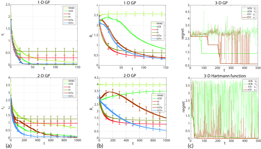
We sampled 200 functions from a 1-D GP and 100 functions from a 2-D GP with known priors (Matérn kernel and linear mean function). The maximum number of rounds was 150 for 1-D and 1000 for 2-D. The first samples were the same for all the methods to minimize randomness effects. Table 1 shows the lowest simple regret achieved ($r_{\min}$) and the number of rounds needed to reach it ($T_{\min}$). We measure the mean ($\bar{T}_{\min}$ and $\bar{r}_{\min}$) and the median ($\hat{T}_{\min}$ and $\hat{r}_{\min}$). Figure 1(a) illustrates the average simple regret and the standard deviation (scaled by $1/4$). While the progress of EI and PI quickly levels off, the other methods continue to reduce the regret, ESTn being the fastest. Moreover, the standard deviation of ESTa and ESTn is much lower than that of PI and EI. Rand is inferior both in terms of $T_{\min}$ and $r_{\min}$. UCB finds a good point but takes more than twice as many rounds as EST for doing so.

Table 1: Minimum Regret $r(t)$ and time to achieve this minimum for functions sampled from 1-D (top) and 2-D Gaussian Processes (bottom) with a limited budget of iterations. ESTa and ESTn achieve lower regret values ($r_{\min}$) faster than other methods ($T_{\min}$). Here, ‘¯’ denotes the mean and ‘^’ the median.

1-D GP, max 150 rounds
	RAND	UCB	EI	PI	ESTa	ESTn
$\hat{T}_{min}$	79.5	53	8	7	26	23
$\hat{r}_{min}$	0.051	0.000	0.088	0.487	0.000	0.000
$\bar{T}_{min}$	78.4	50.9	9.77	8.32	26.1	21.9
$\bar{r}_{min}$	0.107	0.000	0.295	0.562	0.024	0.043
2-D GP, max 1000 rounds
	RAND	UCB	EI	PI	ESTa	ESTn
$\hat{T}_{\min}$	450.5	641.5	40.5	45	407.5	181
$\hat{r}_{\min}$	0.640	0.090	1.035	1.290	0.000	0.000
$\bar{T}_{\min}$	496.3	573.8	48.4	59.8	420.7	213.4
$\bar{r}_{\min}$	0.671	0.108	0.976	1.26	0.021	0.085

Figure 1(b) shows the cumulative regret $R_{T}$. As for the simple regret, we see that EI and PI focus too much on exploitation, stalling at a suboptimal point. EST converges to lower values, and faster than UCB. For additional intuition on cumulative regret, Figure 1(c) plots the cumulative regret $\tilde{r}_{t}$ and the simple regret $r_{t}$ for UCB and EST for a function sampled from 3-D GP and a standard optimization test function (the 3-D Hartmann function). UCB tends to have higher cumulative regret than other methods because it keeps exploring drastically even after having reached the optimum of the function. This observation is in agreement with the experimental results in [30] (they improved UCB’s performance by scaling $\lambda_{t}$ down by a factor of 5), indicating that the scheme of setting $\lambda_{t}$ in UCB is not always ideal in practice.

In summary, the results for synthetic functions suggest that throughout, compared to other methods, EST finds better function values within a smaller number of iterations.

4.2 Initialization Tuning for Trajectory Optimization

In online planning, robots must make a decision quickly, within a possibly unknown budget (humans can stop the “thinking period” of the robot any time, asking for a feasible and good decision to execute). We consider the problem of trajectory optimization, a non-convex optimization problem that is commonly solved via sequential quadratic programming (SQP) [27]. The employed solvers suffer from sub-optimal local optima, and, in real-world scenarios, even merely reaching a feasible solution can be challenging. Hence, we use Bayesian Optimization to tune the initialization for trajectory optimization. In this setting, ${\bm{x}}$ is a trajectory initialization, and $f({\bm{x}})$ the score of the solution returned by the solver after starting it at ${\bm{x}}$.

Table 2: Lowest reward attained in 20 rounds on the airplane problem (illustrated in Figure 2). The results are averages over 8 settings.

	RAND	UCB	EI
mean	27.4429	29.2021	29.1832
std	3.3962	3.1247	3.1377
	PI	ESTa	ESTn
mean	28.0214	27.7587	29.2071
std	4.1489	4.2783	3.1171

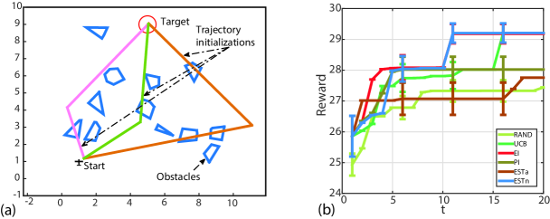
Our test example is the 2D airplane problem from [32], illustrated in Figure 2. We used 8 configurations of the starting point and fixed the target. Our candidate set $\mathfrak{X}$ of initializations is a grid of the first two dimensions of the midpoint state of the trajectory (we do not optimize over speed here). To solve the SQP, we used SNOPT [9]. Figure 2 shows the maximum rewards achieved up to round $t$ (standard deviations scaled by 0.1), and Table 2 displays the final rewards. ESTn achieves rewards on par with the best competitors. Importantly, we observe that Bayesian optimization achieves much better results than the standard random restarts, indicating a new successful application of Bayesian optimization.

Figure 2: (a) Illustration of trajectory initializations. Trajectory initializations are passed to the non-convex optimization solver to ensure a solution with as few collisions with the obstacles as possible. (b) Maximum rewards up to round $t$. EI and ESTn perform relatively better than other methods.

4.3 Parameter Tuning for Image Classification

Our third set of experiments addresses Bayesian optimization for efficiently tuning parameters in visual classification tasks. Here, ${\bm{x}}$ is the model parameter and $y$ the accuracy on the validation set. Our six image datasets are standard benchmarks for object classification (Caltech101 [8] and Caltech256 [10]), scene classification (Indoor67 [23] and SUN397 [35]), and action/event classification (Action40 [36] and Event8 [18]). The number of images per data set varies from 1,500 to 100,000. We use deep CNN features pre-trained on ImageNet [14], the state of the art on various visual classification tasks [25].

Our experimental setup follows [37]. The data is split into training, validation (20% of the original training set) and test set following the standard settings of the datasets. We train a linear SVM using the deep features, and tune its regularization parameter $C$ via Bayesian optimization on the validation set. After obtaining the parameter recommended by each method, we train the classifier on the whole training set, and then evaluate on the test set.

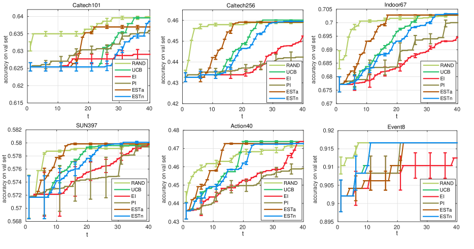
Figure 3 shows the maximum achieved accuracy on the validation set during the iterations of Bayesian optimization on the six datasets. While all methods improve the classification accuracy, ESTa does so faster than other methods. Here too, PI and EI seem to explore too little.

Figure 3: Maximum accuracy on the validation set over the iteration of the optimization. ESTa converges faster than other methods. Experiments are repeated 5 times, the standard deviation is scaled by 1/4.

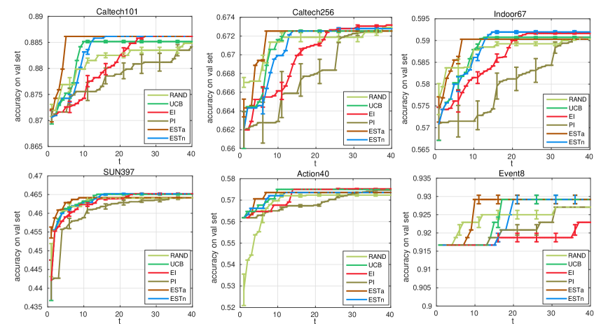
Table 3 displays the accuracy on the test set using the best parameter found by ESTa and ESTn, indicating that the parameter tuning via EST improved classification accuracy. For example, the tuning improves the accuracy on Action40 and SUN397 by 3-4% over the results in [37].

Table 3: Classification accuracy for visual classification on the test set after the model parameter is tuned. Tuning achieves good improvements over the results in [37].

	Caltech101	Caltech256	Indoor67
[37]	87.22	67.23	56.79
ESTa	88.23	69.39	60.02
ESTn	88.25	69.39	60.08
	SUN397	Action40	Event8
[37]	42.61	54.92	94.42
ESTa	47.13	57.60	94.91
ESTn	47.21	57.58	94.86

5 Discussion

Next, we discuss a few further details and extensions.

Setting $\hat{m}$.

In Section 2, we discussed one way of setting $\hat{m}$. There, we used an approximation with independent variables. We focused on Equations (3) and (4) throughout the paper since they yield upper bounds $\hat{m}\geq m$ that preserve our theoretical results. Nevertheless, other possibilities for setting $\hat{m}$ are conceivable. For example, close in spirit to Thompson and importance sampling, one may sample $\hat{m}$ from $\Pr[Y]=\prod_{{\bm{x}}\in\mathfrak{X}}\Phi(\frac{Y-\mu({\bm{x}})}{\sigma({\bm{x}})})$. Furthermore, other search strategies can be used, such as guessing or doubling, and prior knowledge about properties of $f$ such as the range can be taken into account.

Discretization.

In our approximations, we used discretizations of the input space. While adding a bit more detail about this step here, we focus on the noiseless case, described by Equation (4). Equation (3) can be analyzed similarly for more general settings. For a Lipschitz continuous function, it is essentially sufficient to estimate the probability of $f({\bm{x}})\leq y,\forall{\bm{x}}\in\mathfrak{X}$ on set $\mathfrak{W}$, which is a $\rho$-covering of $\mathfrak{X}$.

We assume that $f$ is Lipschitz continuous. Our analysis can be adapted to the milder assumption that $f$ is Lipschitz continuous with high probability. Let $L$ be the Lipschitz constant of $f$. By assumption, we have $|f({\bm{x}})-f({\bm{x}}^{\prime})|\leq L\rho$, for all $\|{\bm{x}}-{\bm{x}}^{\prime}\|\leq\rho.$ If $\mathfrak{X}$ is a continuous set, we construct its $\rho$-covering $\mathfrak{W}$ such that $\forall{\bm{x}}\in\mathfrak{X}$, $\inf_{{\bm{x}}^{\prime}\in\mathfrak{W}}\|{\bm{x}}-{\bm{x}}^{\prime}\|\leq\rho$. Let $E_{\mathfrak{X}}(y)$ be the event that $f({\bm{x}})\leq y,\forall{\bm{x}}\in\mathfrak{X}$. Then, $\Pr[E_{\mathfrak{X}}(y)]\geq\Pr[E_{\mathfrak{W}}(y-\rho L),E_{\mathfrak{X}\setminus\mathfrak{W}}(y)]=\Pr[E_{\mathfrak{W}}(y-\rho L)]$ The last step uses Lipschitz continuity to compute $\Pr[E_{\mathfrak{X}\setminus\mathfrak{W}}(y)|[E_{\mathfrak{W}}(y-\rho L)]=1$. We can use this lower bound to compute $\hat{m}$, so $\hat{m}$ remains an upper bound on $m$. Notably, none of the regret bounds relies on a discretization of the space. Morever, once $\hat{m}$ is chosen, the acquisition function can be optimized with any search method, including gradient descent.

High dimensions.

Bayesian Optimization methods generally suffer in high dimensions. Common assumptions are a low-dimensional or simpler underlying structure of $f$ [7, 34, 15]. Our approach can be combined with those methods too, to be extended to higher dimensions.

Relation to entropy search.

EST is closely related to entropy search (ES) methods [12, 13], but also differs in a few important aspects. Like EST, ES methods approximate the probability of a point ${\bm{x}}$ being the maximizer $\operatorname{arg\,max}_{{\bm{x}}^{\prime}\in\mathfrak{X}}f({\bm{x}}^{\prime})$, and then choose where to evaluate next by optimizing an acquisition function related to this probability. However, instead of choosing the input that is most likely to be the $\operatorname{arg\,max}$, ES chooses where to evaluate next by optimizing the expected change in the entropy of $\Pr[M_{\bm{x}}]$. One reason is that ES does not aim to minimize cumulative regret like many other bandit methods (including EST). The cumulative regret penalizes all queried points, and a method that minimizes the cumulative regret needs to query enough supposedly good points. ES methods, in contrast, purely focus on exploration, since their objective is to gather as much information as possible to estimate a final value in the very end. Since the focus of this work lies on cumulative regret, detailed empirical comparisons between EST and ES may be found in the supplement.

6 Conclusion

In this paper, we studied a new Bayesian optimization strategy derived from the viewpoint of the estimating the $\operatorname{arg\,max}$ of an unknown function. We showed that this strategy corresponds to adaptively setting the trade-off parameters $\lambda$ and $\theta$ in GP-UCB and GP-PI, and established bounds on the regret. Our experiments demonstrate that this strategy is not only easy to use, but robustly performs well by measure of different types of regret, on a variety of real-world tasks from robotics and computer vision.

Acknowledgements.

We thank Leslie Kaelbling and Tomás Lozano-Pérez for discussions, and Antonio Torralba for support with computational resources. We gratefully acknowledge support from NSF CAREER award 1553284, NSF grants 1420927 and 1523767, from ONR grant N00014-14-1-0486, and from ARO grant W911NF1410433. Any opinions, findings, and conclusions or recommendations expressed in this material are those of the authors and do not necessarily reflect the views of our sponsors.

Supplement

In this supplement, we provide proofs for all theorems and lemmas in the main paper, more exhaustive experimental results and details on the experiments.

Appendix A Proofs

A.1 Proofs from Section 2

See 2.1

Proof.

We omit the subscripts $t$ for simplicity. Let $\bm{a}$ be the point selected by GP-UCB, and $\bm{b}$ selected by EST. Without loss of generality, we assume $\bm{a}$ and $\bm{b}$ are unique. With $\lambda=\min_{{\bm{x}}\in\mathfrak{X}}\frac{\hat{m}-\mu({\bm{x}})}{\sigma({\bm{x}})}$, GP-UCB chooses to evaluate

$$\bm{a}=\operatorname{arg\,max}_{{\bm{x}}\in\mathfrak{X}}\mu({\bm{x}})+\lambda\sigma({\bm{x}})=\operatorname{arg\,min}_{{\bm{x}}\in\mathfrak{X}}\frac{\hat{m}-\mu({\bm{x}})}{\sigma({\bm{x}})}.$$

This is because

$$\hat{m}=\max_{{\bm{x}}\in\mathfrak{X}}\mu({\bm{x}})+\lambda\sigma({\bm{x}})=\mu(\bm{a})+\lambda\sigma(\bm{a}).$$

By definition of $\bm{b}$, for all ${\bm{x}}\in\mathfrak{X}$, we have

$$\frac{\Pr[M_{\bm{b}}|\hat{m},\mathfrak{D}]}{\Pr[M_{\bm{x}}|\hat{m},\mathfrak{D}]} \approx\frac{Q(\frac{\hat{m}-\mu(\bm{b})}{\sigma(\bm{b})})\prod_{{\bm{x}}^{\prime}\neq\bm{b}}\Phi(\frac{\hat{m}-\mu({\bm{x}}^{\prime})}{\sigma({\bm{x}}^{\prime})})}{Q(\frac{\hat{m}-\mu({\bm{x}})}{\sigma({\bm{x}})})\prod_{{\bm{x}}^{\prime}\neq{\bm{x}}}\Phi(\frac{\hat{m}-\mu({\bm{x}}^{\prime})}{\sigma({\bm{x}}^{\prime})})}$$

$$=\frac{Q(\frac{\hat{m}-\mu(\bm{b})}{\sigma(\bm{b})})\Phi(\frac{\hat{m}-\mu({\bm{x}})}{\sigma({\bm{x}})})}{Q(\frac{\hat{m}-\mu({\bm{x}})}{\sigma({\bm{x}})})\Phi(\frac{\hat{m}-\mu(\bm{b})}{\sigma(\bm{b})})}$$

$$\geq 1.$$

The inequality holds if and only if $\frac{\hat{m}-\mu(\bm{b})}{\sigma(\bm{b})}\leq\frac{\hat{m}-\mu({\bm{x}})}{\sigma({\bm{x}})}$ for all ${\bm{x}}\in\mathfrak{X}$, including $\bm{a}$, and hence

$$\frac{\hat{m}-\mu(\bm{b})}{\sigma(\bm{b})}\leq\frac{\hat{m}-\mu(\bm{a})}{\sigma(\bm{a})}=\lambda=\min_{{\bm{x}}\in\mathfrak{X}}\frac{\hat{m}-\mu({\bm{x}})}{\sigma({\bm{x}})},$$

which, with uniqueness, implies that $\bm{a}=\bm{b}$ and GP-UCB and EST select the same point.

For the other direction, we denote the candidate selected by GP-UCB by

$$\bm{a}=\operatorname{arg\,max}_{{\bm{x}}\in\mathfrak{X}}{\mu({\bm{x}})+\lambda\sigma({\bm{x}})}.$$

The variant of EST with $\hat{m}=\max_{{\bm{x}}\in\mathfrak{X}}{\mu({\bm{x}})+\lambda\sigma({\bm{x}})}$ selects

$$\bm{b}=\operatorname{arg\,max}_{{\bm{x}}\in\mathfrak{X}}\Pr[M_{{\bm{x}}}|\hat{m},\mathfrak{D}].$$

We know that for all ${\bm{x}}\in\mathfrak{X}$, we have $\frac{\hat{m}-\mu(\bm{b})}{\sigma(\bm{b})}\leq\frac{\hat{m}-\mu({\bm{x}})}{\sigma({\bm{x}})}$ and hence $\hat{m}\leq\mu(\bm{b})+\frac{\hat{m}-\mu({\bm{x}})}{\sigma({\bm{x}})}\sigma(\bm{b})$. Since $\hat{m}=\mu(\bm{a})+\lambda\sigma(\bm{a})$, letting ${\bm{x}}=\bm{a}$ implies that

$$\hat{m}=\max_{{\bm{x}}\in\mathfrak{X}}{\mu({\bm{x}})+\lambda\sigma({\bm{x}})}\leq\mu(\bm{b})+\lambda\sigma(\bm{b}).$$

Hence, by uniqueness it must be that $\bm{a}=\bm{b}$ and GP-UCB and EST select the same candidate. ∎

A.2 Proofs from Section 3

See 3.2

Proof.

Let $z_{t}=\frac{\mu_{t-1}(x_{t})-f(x_{t})}{\sigma_{t-1}(x_{t})}\sim\mathcal{N}(0,1)$. It holds that

$$\Pr[z_{t}>\zeta_{t}] =\int_{\zeta_{t}}^{+\infty}\frac{1}{\sqrt{2\pi}}e^{-z^{2}/2}\mathop{}\!\mathrm{d}z$$

$$=\int_{\zeta_{t}}^{+\infty}\frac{1}{\sqrt{2\pi}}e^{-(z-\zeta_{t})^{2}/2-\zeta_{t}^{2}/2-z\zeta_{t}}\mathop{}\!\mathrm{d}z$$

$$\leq e^{-\zeta_{t}^{2}/2}\int_{\zeta_{t}}^{+\infty}\frac{1}{\sqrt{2\pi}}e^{-(z-\zeta_{t})^{2}/2}\mathop{}\!\mathrm{d}z$$

$$=\frac{1}{2}e^{-\zeta_{t}^{2}/2}.$$

A union bound extends this bound to all rounds:

$$\Pr[z_{t}>\zeta_{t}\text{ for some }t\in[1,T]]\leq\sum_{t=1}^{T}\frac{1}{2}e^{-\zeta_{t}^{2}/2}.$$

With $\zeta_{t}=(2\log(\frac{\pi_{t}}{2\delta}))^{\frac{1}{2}}$ and $\sum_{t=1}^{T}\pi_{t}^{-1}=1$, this implies that with probability at least $1-\delta$, it holds that $\mu_{t-1}({\bm{x}}_{t})-f({\bm{x}}_{t})\leq\zeta_{t}\sigma_{t-1}({\bm{x}}_{t})$ for all $t\in[1,T]$. One may set $\pi_{t}=\tfrac{1}{6}\pi^{2}t^{2}$, or $\pi_{t}=T$, in which case $\zeta_{t}=\zeta=(2\log(\frac{T}{2\delta}))^{\frac{1}{2}}$. ∎

See 3.3

Proof.

At time step $t\geq 1$, we have

$$\tilde{r}_{t} =\max_{{\bm{x}}\in\mathfrak{X}}f({\bm{x}})-f({\bm{x}}_{t})$$

$$\leq\hat{m}_{t}-f({\bm{x}}_{t})$$

$$\leq\hat{m}_{t}-\mu_{t-1}({\bm{x}}_{t})+\zeta_{t}\sigma_{t-1}({\bm{x}}_{t})$$

$$=(\nu_{t}+\zeta_{t})\sigma_{t-1}({\bm{x}}_{t}).$$

∎

Appendix B Experiments

B.1 Approximate $m$

In the paper, we estimate $m$ to be

$$\hat{m}=m_{0}+\int_{m_{0}}^{\infty}1-\prod_{{\bm{x}}\in\mathfrak{W}}\Phi\Big{(}\frac{w-\mu({\bm{x}})}{\sigma({\bm{x}})}\Big{)}\mathop{}\!\mathrm{d}w$$

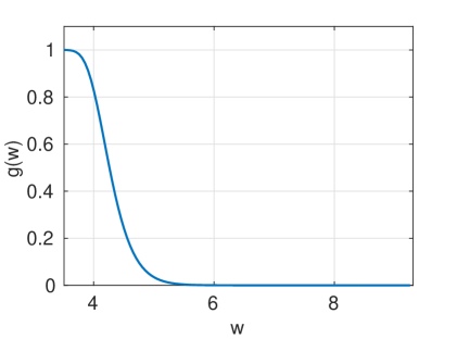
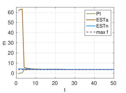
which involves an integration from the current maximum $m_{0}$ of the observed data to positive infinity. In fact the factor inside the integration quickly approaches zero in practice. We plot $g(w)=1-\prod_{{\bm{x}}\in\mathfrak{W}}\Phi\Big{(}\frac{w-\mu({\bm{x}})}{\sigma({\bm{x}})}\Big{)}$ in Figure 4, which looks like half of a Gaussian distribution. So instead of numerical integration (which can be done efficiently), heuristically we can sample two values of $g(w)$ to fit $\hat{g}(w)=ae^{-(w-m_{0})^{2}/2b^{2}}$ and do the integration $\int_{m_{0}}^{\infty}\hat{g}(w)\mathop{}\!\mathrm{d}w=\sqrt{2\pi}ab$ analytically to be more efficient. This method is what we called ESTa in the paper, while the numerical integration is called ESTn.

We notice that our estimation $\hat{m}$ can serve as a tight upper bound on the real value of the max of the function in practice. One example of is shown in Figure 4 with a 1-D GP function. This example shows how PI, ESTa and ESTn estimate $m$. Both ESTa and ESTn are upper bounds of the true maximum of the function, and ESTn is actually very tight. For PI, $\theta=\operatorname{arg\,max}_{1\leq\tau<t}y_{\tau}+\epsilon$ is always a lower bound of an $\epsilon$ shift over the true maximum of the function.

Figure 4: Top: $g(w)$, $w\in[m_{0},+\infty)$; Bottom: estimation of $m$.

Figure 5: Examples of a function sampled from 1-D GP (top), and a function sampled from 2-D GP (bottom) with isotropic Matérn kernel and linear mean function. We deliberately create many local optimums to make the problem hard.

B.2 Synthetic data

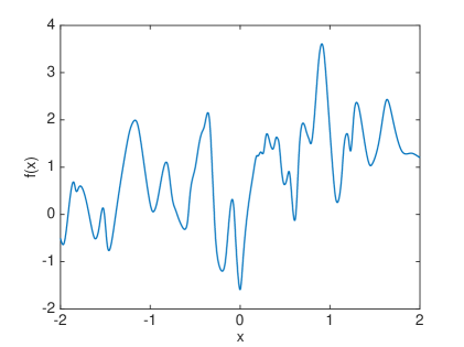
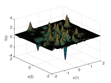
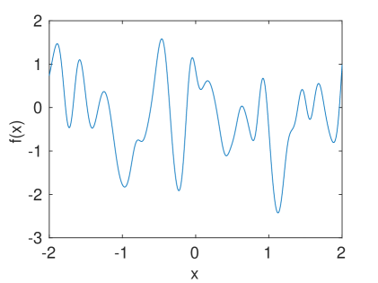
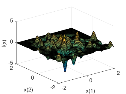
We show the examples of the functions we sampled from GP in Figure 5. The covariance function of GP is an isotropic Matérn kernel with parameters $\ell=0.1,\sigma_{f}=1$. The mean function is a linear function with a fixed random slope for different dimensions, and the constant is $1$.

B.3 Initialization tuning for trajectory optimization

The 8 configurations of start state are $[7\;1\;0\;0]$, $[7\;0\;0\;0]$, $[1\;0\;0\;0]$, $[1\;1\;0\;0]$, $[2\;0\;0\;0]$, $[2\;1\;0\;0]$, $[3\;0\;0\;0]$, $[3\;1\;0\;0]$, where the first two dimensions denote the position and the last two dimension denote the speed. We only tune the first two dimension and keep the speed to be 0 for both directions. The target state is fixed to be $[5\;9\;0\;0]$.

We can initialize the trajectory by setting the mid point of trajectory to be any point falling on the grid of the space (both x axis and y axis have range $[-2,12]$). Then use SNOPT to solve the trajectory optimization problem, which involves an objective cost function (we take the negative cost to be a reward function to maximize), dynamics constraints, and obstacle constraints etc. Details of trajectory optimization are available in [32, 31].

We used the same settings of parameters for GP as in Section B.2 for all the methods we tested and did kernel parameter fitting every 5 rounds. The same strategy was used for the image classification experiments in the next section.

B.4 Parameter tuning for image classification

We use the linear SVM in the liblinear package for all the image classification experiments. We extract the FC7 activation from the imagenet reference network in the Caffe deep learning package [14] as the visual feature. The reported classification accuracy is the accuracy averaged over all the categories. ‘-c’ cost is the model parameter we tune for the linear SVM.

In Caltech101 and Caltech256 experiment [8, 10], there are 8,677 images from 101 object categories in the Caltech101 and 29,780 images from 256 object categories. The training size is 30 images per category, and the rest are test images.

In SUN397 experiment [35], there are 108,754 images from 397 scene categories. Images are randomly split into training and test set. The training size is 50 images per category, and the rest are test images.

In MIT Indoor67 experiment [23], there are 15,620 images from 67 indoor scene categories. Images are randomly split into training set and test set. The training size is 100 images per category, and the rest are test images.

In Stanford Action40 experiment [36], there are 9,532 images from 40 action categories. Images are randomly split into training set and test set. The training size is 100 images per category, and the rest are test images.

In UIUC Event8 experiment [18], there are 1,579 images from 8 event categories. Images are randomly split into training set and test set. Training size is 70 images per category, and the rest are test images.

We used features extracted from a convolutional neural network (CNN) that was trained on images from ImageNet. It has been found [37] that features from a CNN trained on a set of images focused more on places than on objects, the Places database, work better in some domains. So, we repeated our experiments using the Places-CNN features, and the results are shown in Figure 6 and Table 4. All the methods help to improve the classification accuracy on the validation set. EST methods achieve good accuracy on each validation set on par with the best competitors for most of the datasets. And we also observe that for Caltech101 and Event8, Rand and UCB converge faster and achieve better accuracy than other methods. As we have shown in Section 4.1, UCB and Rand perform worse than other methods in terms of cumulative regret, because they tend to explore too much. However, more exploration can be helpful for some black-box functions that do not satisfy our assumption that they are samples from GP. For example, for discontinuous step functions, pure exploration can be beneficial for simple regret. One possible explanation for the better results of Rand and UCB is that the black-box functions we optimize here are possibly functions not satisfying our assumption. The strong assumption on the black-box function is also a major drawback of Bayesian optimization,

Figure 6: Maximum accuracy on the validation set over iteration of the optimization. Experiments are repeated 5 times. The visual features used here are Deep CNN features pre-trained on the Places database.

Table 4: Classification accuracy on the test set of the datasets after the model parameter is tuned by ESTa and ESTn. Tuning achieves good improvement over the results in [37].

	Caltech101	Caltech256	Indoor67	SUN397	Action40	Event8
Imagenet-CNN feature	87.22	67.23	56.79	42.61	54.92	94.42
ESTa	88.23	69.39	60.02	47.13	57.60	94.91
ESTn	88.25	69.39	60.08	47.21	57.58	94.86
Places-CNN feature	65.18	45.59	68.24	54.32	42.86	94.12
ESTa	66.94	47.51	70.27	58.57	46.24	93.79
ESTn	66.95	47.43	70.27	58.65	46.17	93.56

B.5 Comparison to entropy search methods

Entropy search methods [12, 13] aim to minimize the entropy of the probability for the event $M_{{\bm{x}}}$ (${\bm{x}}=\operatorname{arg\,max}_{{\bm{x}}^{\prime}\in\mathfrak{X}}f({\bm{x}}^{\prime})$). Although not suitable for minimizing cumulative regret, ES methods are intuitively ideal for minimizing simple regret. We hence in this section compare the empirical performance of entropy search (ES) [12] and predictive entropy search (PES) [13] to that of the EST methods (EST/GP-UCB/PI) and EI.

Since both ES and PES only support squared exponential covariance function and zero mean function in their code right now, and it requires significant changes in their code to accommodate other covariance functions, we created synthetic functions that are different from the ones we used in Section 4 in the paper. The new functions are sampled from 1-D (80 functions) and 2-D GP (20 functions) with squared exponential kernel ($\sigma_{f}=0.1$ and $l=1$) and 0 mean. Function examples are shown in Figure 9.

Figure 7: Simple regret for functions sampled from 1-D GP with squared exponential kernel and 0 mean.

Figure 8: Simple regret for functions sampled from 2-D GP with squared exponential kernel and 0 mean.

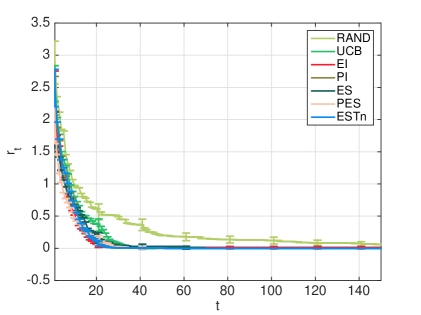
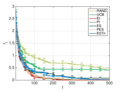
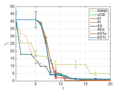
We show the results on these synthetic functions in Figure 7,8, and a standard optimization test function, Branin Hoo function, in Figure 10. It is worth noting that ES methods make queries on the most informative points, which are not necessarily the points with low regret. At each round, ES methods make a “query” on the black-box function, and then make a “guess” of the $\operatorname{arg\,max}$ of the function (but do not test the “guess”). We plot the regret achieved by the “guesses” made by ES methods. For the 1-D GP task, all the methods behave similarly and achieve zero regret except Rand. For the 2-D GP task, EI is the fastest method to converge to zero regret, and in the end ESTn, PI,EI and ES methods achieve similar results. For the test on Branin Hoo function, PES achieves the lowest regret. ESTa converges slightly faster than PES, but to a slightly higher regret.

Figure 9: Examples of a function sampled from 1-D GP (left), and a function sampled from 2-D GP (right) with squared exponential kernel and 0 mean functions. These functions can be easier than the ones in Figure 5 since they have fewer local optima.

Figure 10: Simple regret for Branin Hoo function. UCB/EI/PI/ESTa/ESTn use the isotropic Matérn kernel with parameters $\ell=0.1,\sigma_{f}=1$; ES/PES use the isotropic squared exponential kernel with $\ell=0.1,\sigma_{f}=1$.

We also compared the running time for all the methods in Table 5. It is assumed in GP optimization that it is more expensive to evaluate the blackbox function than computing the next query to evaluate using GP optimization techniques. However, in practice, we still want the algorithm to output the next query point as soon as possible. For ES methods, it can be sometimes unacceptable to run them for black-box functions that take minutes to complete a query.

Table 5: Comparison on the running time (s) per iteration.

RAND	UCB	EI	PI
0.0002	0.075	0.079	0.076
ESTa	ESTn	ES	PES
0.078	0.55	56	106

References

- Auer [2002] P. Auer. Using confidence bounds for exploitation-exploration tradeoffs. Journal of Machine Learning Research, 3:397–422, 2002.
- Auer et al. [2002] P. Auer, N. Cesa-Bianchi, and P. Fischer. Finite-time analysis of the multiarmed bandit problem. Machine learning, 47(2-3):235–256, 2002.
- Brochu et al. [2009] E. Brochu, V. M. Cora, and N. De Freitas. A tutorial on Bayesian optimization of expensive cost functions, with application to active user modeling and hierarchical reinforcement learning. Technical Report TR-2009-023, University of British Columbia, 2009.
- Bubeck et al. [2009] S. Bubeck, R. Munos, and G. Stoltz. Pure exploration in multi-armed bandits problems. In Algorithmic Learning Theory, pages 23–37. Springer, 2009.
- Bull [2011] A. D. Bull. Convergence rates of efficient global optimization algorithms. Journal of Machine Learning Research, 12:2879–2904, 2011.
- Calandra et al. [2014] R. Calandra, A. Seyfarth, J. Peters, and M. P. Deisenroth. An experimental comparison of Bayesian optimization for bipedal locomotion. In International Conference on Robotics and Automation (ICRA), 2014.
- Djolonga et al. [2013] J. Djolonga, A. Krause, and V. Cevher. High-dimensional Gaussian process bandits. In Advances in Neural Information Processing Systems (NIPS), 2013.
- Fei-Fei et al. [2007] L. Fei-Fei, R. Fergus, and P. Perona. Learning generative visual models from few training examples: An incremental Bayesian approach tested on 101 object categories. Computer Vision and Image Understanding, 2007.
- Gill et al. [2002] P. E. Gill, W. Murray, and M. A. Saunders. SNOPT: An SQP algorithm for large-scale constrained optimization. SIAM Journal on optimization, 12(4):979–1006, 2002.
- Griffin et al. [2007] G. Griffin, A. Holub, and P. Perona. Caltech-256 object category dataset. Technical Report 7694, California Institute of Technology, 2007.
- Grünewälder et al. [2010] S. Grünewälder, J.-Y. Audibert, M. Opper, and J. Shawe-Taylor. Regret bounds for Gaussian process bandit problems. In International Conference on Artificial Intelligence and Statistics (AISTATS), 2010.
- Hennig and Schuler [2012] P. Hennig and C. J. Schuler. Entropy search for information-efficient global optimization. Journal of Machine Learning Research, 13:1809–1837, 2012.
- Hernández-Lobato et al. [2014] J. M. Hernández-Lobato, M. W. Hoffman, and Z. Ghahramani. Predictive entropy search for efficient global optimization of black-box functions. In Advances in Neural Information Processing Systems (NIPS), 2014.
- Jia [2013] Y. Jia. Caffe: An open source convolutional architecture for fast feature embedding. http://caffe.berkeleyvision.org/, 2013.
- Kandasamy et al. [2015] K. Kandasamy, J. Schneider, and B. Poczos. High dimensional Bayesian optimisation and bandits via additive models. In International Conference on Machine Learning (ICML), 2015.
- Krause and Ong [2011] A. Krause and C. S. Ong. Contextual Gaussian process bandit optimization. In Advances in Neural Information Processing Systems (NIPS), 2011.
- Kushner [1964] H. J. Kushner. A new method of locating the maximum point of an arbitrary multipeak curve in the presence of noise. Journal of Fluids Engineering, 86(1):97–106, 1964.
- Li and Fei-Fei [2007] L.-J. Li and L. Fei-Fei. What, where and who? classifying events by scene and object recognition. In International Conference on Computer Vision (ICCV), 2007.
- Lizotte et al. [2007] D. J. Lizotte, T. Wang, M. H. Bowling, and D. Schuurmans. Automatic gait optimization with Gaussian process regression. In International Conference on Artificial Intelligence (IJCAI), 2007.
- Lizotte et al. [2012] D. J. Lizotte, R. Greiner, and D. Schuurmans. An experimental methodology for response surface optimization methods. Journal of Global Optimization, 53(4):699–736, 2012.
- Massart [2007] P. Massart. Concentration Inequalities and Model Selection, volume 6. Springer, 2007.
- Moc̆kus [1974] J. Moc̆kus. On Bayesian methods for seeking the extremum. In Optimization Techniques IFIP Technical Conference, 1974.
- Quattoni and Torralba [2009] A. Quattoni and A. Torralba. Recognizing indoor scenes. In IEEE Conference on Computer Vision and Pattern Recognition (CVPR), 2009.
- Rasmussen and Williams [2006] C. E. Rasmussen and C. K. Williams. Gaussian processes for machine learning. The MIT Press, 2006.
- Razavian et al. [2014] A. S. Razavian, H. Azizpour, J. Sullivan, and S. Carlsson. CNN features off-the-shelf: an astounding baseline for recognition. In IEEE Conference on Computer Vision and Pattern Recognition (CVPR), 2014.
- Ross [2003] A. M. Ross. Useful bounds on the expected maximum of correlated normal variables. Technical report, Technical Report 03W-004, ISE Dept., Lehigh Univ., Aug, 2003.
- Schulman et al. [2013] J. Schulman, J. Ho, A. Lee, I. Awwal, H. Bradlow, and P. Abbeel. Finding locally optimal, collision-free trajectories with sequential convex optimization. In Robotics: Science and Systems Conference (RSS), volume 9, pages 1–10, 2013.
- Slepian [1962] D. Slepian. The one-sided barrier problem for Gaussian noise. Bell System Technical Journal, 41(2):463–501, 1962.
- Snoek et al. [2012] J. Snoek, H. Larochelle, and R. P. Adams. Practical Bayesian optimization of machine learning algorithms. In Advances in Neural Information Processing Systems (NIPS), 2012.
- Srinivas et al. [2010] N. Srinivas, A. Krause, S. M. Kakade, and M. Seeger. Gaussian process optimization in the bandit setting: No regret and experimental design. In International Conference on Machine Learning (ICML), 2010.
- [31] R. Tedrake. Underactuated Robotics: Algorithms for Walking, Running, Swimming, Flying, and Manipulation (Course Notes for MIT 6.832). Downloaded in Fall, 2014 from http://people.csail.mit.edu/russt/underactuated/.
- Tedrake [2014] R. Tedrake. Drake: A planning, control, and analysis toolbox for nonlinear dynamical systems. http://drake.mit.edu, 2014.
- Thornton et al. [2013] C. Thornton, F. Hutter, H. H. Hoos, and K. Leyton-Brown. Auto-WEKA: combined selection and hyperparameter optimization of classification algorithms. In ACM SIGKDD Conference on Knowledge Discovery and Data Mining (KDD), 2013.
- Wang et al. [2013] Z. Wang, M. Zoghi, F. Hutter, D. Matheson, and N. De Freitas. Bayesian optimization in high dimensions via random embeddings. In International Conference on Artificial Intelligence (IJCAI), 2013.
- Xiao et al. [2010] J. Xiao, J. Hays, K. A. Ehinger, A. Oliva, and A. Torralba. Sun database: large-scale scene recognition from abbey to zoo. In IEEE Conference on Computer Vision and Pattern Recognition (CVPR), 2010.
- Yao et al. [2011] B. Yao, X. Jiang, A. Khosla, A. L. Lin, L. Guibas, and L. Fei-Fei. Human action recognition by learning bases of action attributes and parts. In International Conference on Computer Vision (ICCV), 2011.
- Zhou et al. [2014] B. Zhou, A. Lapedriza, J. Xiao, A. Torralba, and A. Oliva. Learning deep features for scene recognition using places database. In Advances in Neural Information Processing Systems (NIPS), 2014.