A note on the best invariant estimation of continuous probability distributions
under mean square loss

Abstract

We consider the nonparametric estimation problem of continuous probability distribution functions. For the integrated mean square error we provide the statistic corresponding to the best invariant estimator proposed by Aggarwal Ag55 and Ferguson Fe67 . The table of critical values is computed and a numerical power comparison of the statistic with the traditional Cramér-von Mises statistic is done for several representative distributions.

In 1933, Kolmogogov Ko33 formally defined the empirical distribution function $F_{n}(x)$, and then considered how close this would be to the true distribution function $F(x)$ when it is continuous. This contribution introduced the use of $F_{n}(x)$ as an estimator of $F(x)$, to be followed by its use in testing a given $F(x)$. Modifying the statistics proposed earlier by Cramér Cr28 and von Mises Mi31 , Smirnov Sm36 Sm37 compared the hypothesis $F(x)$ with $F_{n}(x)$ by means of the quadratic loss function

$$L=\int_{-\infty}^{\infty}\,(F(x)-F_{n}(x))^{2}\,w(F(x))\,dF(x)$$ (1)

where $w$ is some preassigned positive weight function. Let $x_{1},...,x_{n}$ be a random sample drawn from the continuous probability distribution function $F(x)$ with density function $f(x)$ and let $x_{1}^{*}<x_{2}^{*}<...<x_{n}^{*}$ be obtained by ordering each realization $x_{1},...,x_{n}$. For $w=1$, the expression (1) can be written equivalently as

$$\omega^{2}=\frac{1}{12n^{2}}+\frac{1}{n}\sum\limits_{i=1}^{n}\Big{[}\,F_{i}-\frac{2i-1}{2n}\,\Big{]}^{2}$$ (2)

with $F_{i}=F(x_{i}^{*})$. The term $n\omega^{2}$ is commonly named as the Cramér-von Mises statistic. Smirnov Sm36 Sm37 Sm39 showed that the probability distribution of the latter is independent of $F$ for any $n$ and he obtained an asymptotic expression of its probability distribution for $n\to\infty$. For general weight functions, Anderson and Darling AD52 AD54 presented a general method for obtaining the asymptotic distribution of (1) for $n\to\infty$.

Later on, Aggarwal Ag55 considered a class of invariant loss functions and obtained the best invariant estimators which are also step functions like $F_{n}(x)$. The canonical representation of any invariant estimator is given by

$$\hat{F}(x)=\sum_{i=0}^{n}\hat{F}_{i}\,\textbf{1}_{\nu_{i}}(x)$$ (3)

with real valued factors $0\leq\hat{F}_{i}\leq 1$, $i=0,...,n$, and $\textbf{1}_{\nu_{i}}(x)$ is the indicator function of the set $\nu_{i}$, which is defined by

$$\nu_{0} = (\,-\infty,\,x_{1}^{*}\,)$$

$$\nu_{i} = [\,x_{i}^{*},\,x_{i+1}^{*})\qquad i=1,...,n-1,$$ (4)

$$\nu_{n} = [\,x_{n}^{*},\infty\,).$$

Note that for the empirical distribution, each set $\nu_{i}$ is uniquely corresponding to the particular probability estimate $i/n$, for $i=0,...,n$.
For the risk function

$$R=\text{E}\!\int\,(F-\hat{F})^{2}\,w(F)\,dF$$ (5)

it is known Ag55 Fe67 that

$$\hat{F}(x)=F_{n}(x)$$ (6)

is the best invariant estimate if the weight function is $w(t)=1/t(1-t)$, while the corresponding statistic (1) is given by

$$A^{2}=-1-\frac{1}{n}\sum_{i=1}^{n}\frac{2i-1}{n}\Big{[}\,\log F_{i}+\log(1-F_{n-i+1})\,\Big{]}.$$ (7)

The expression $nA^{2}$ is the commonly denoted Anderson-Darling statistic. On the other hand, it is also known that the estimator

$$\hat{F}(x)=\frac{nF_{n}(x)+1}{n+2}$$ (8)

is best invariant for the ordinary mean square error with $w(t)=1$ in (1). Although the latter can be considered as an improvement of the Cramér-von Mises statistic, it appears that there is no explicit expression of the corresponding statistic given in literature.

Read Re72 pointed out that (6) and (8) can be improved by an estimator which is stochastically smaller than the Kolmogorov statistic. However, the corresponding estimator is not a step function and is not invariant under the full group of strictly increasing transformations as are (6) and (8). Another discussion concerns the admissibility of the estimators (6) and (8). For instance, Yu Yu89a Yu89b Yu89c has shown that (6) is admissible with respect to the weight $w(t)=1/t(1-t)$ only for samples of size $n=1,2$ but inadmissible for samples of size $n\geq 3$. Similarly, for the estimator (8), Brown Br88 has proven inadmissibility for all sample sizes $n\geq 1$. Nevertheless, it is not known if the alternative estimator in Brown’s proof is by itself admissible or whether it is possible to find some other estimator dominating (8) which provides a significantly larger saving in risk from using (8). Therefore, let us provide the following:

Proposition 1. For unit weight $w=1$, the statistic (1) corresponding to the best invariant estimator (8) is

$$\hat{\omega}^{2}=\frac{n+8}{12(n+2)^{3}}+\frac{1}{n+2}\,\sum_{i=1}^{n}\,\Big{[}\,F_{i}-\frac{\,i+\frac{1}{2}}{\,n+2\,}\,\Big{]}^{2}.$$ (9)

Proof. To obtain (9) one has to replace $F_{n}(x)$ in (1) by the estimator (8) and compute the integration. After some algebraic manipulations expression (9) is obtained. $\Box$

The statistic $\hat{\omega}^{2}$ is similar but different from the traditional Cramér-von Mises statistic (2). For large sample sizes they have similar stochastic properties. The minimum risk of the statistic is $1/6(n+2)$, which is slightly less than for the Cramér-von Mises statistic with $1/6n$. Thus, at least for small samples we can expect that (9) will improve (2).

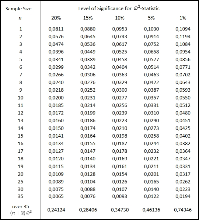
The critical values of (9) are computed by numerical simulation and are provided in the table of Figure 1. For $n=1$, the critical values are $1/3$ of the critical values for the traditional statistic. Moreover, for the 1 percent confidence level the critical values are not strictly monotonic decreasing for increasing sample size. We checked that fact by analytical evaluation for $n=1$ and 2. All quantiles of the table are systematically smaller than for the quantiles of (2). However, that does not necessarily imply that there is an improvement of the type I error against the Cramér-von Mises statistic because for finite sample size $n$ the quantiles of both statistics have different support and the scales are not comparable. Therefore, we compared their statistical power for a few representative examples of distributions $F(x)$, which are supposed to be continuous and completely specified.

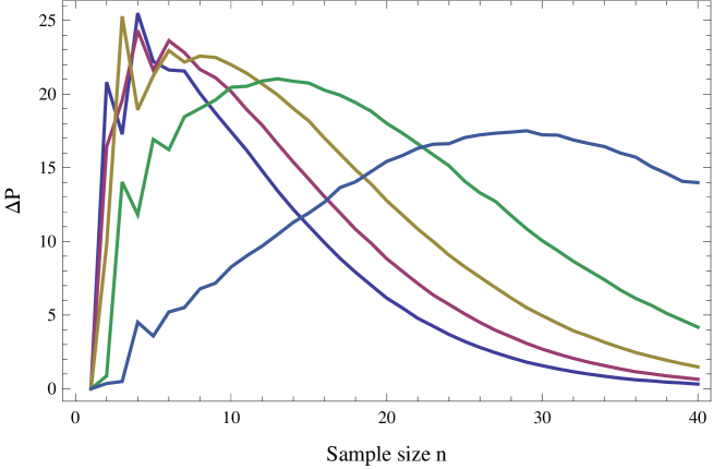
First, we considered the test for normality ($H_{0}$), when $f(x)$ is the uniform distribution ($H_{1}$). In Figure 2, we see the difference $\Delta P$ of the power of (9) and the power of (2), for confidence levels $20,15,10,5$ and $1$ percentage points. The numerical simulation has been performed for $10^{7}$ Monte Carlo steps. For very small and very large samples $n$, the power of both statistics becomes more and more equal. Intermediately, the difference of the power between both grows until 25 percent. For all sample sizes and confidence levels there is a higher power of (9) than for the Cramér and von Mises statistic.

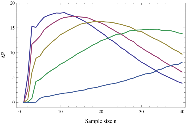
Moreover, we considered the test for uniformity given in Table 3 of Stephens study St74 . When $F(x)$ is completely specified then $F_{i}$ should be uniformly distributed between 0 and 1. The power study has therefore been confined to a test of this hypothesis when $F_{i}$ is drawn from alternative distributions. If the variance of the hypothesized $F(x)$ is correct but the mean is wrong, the $F_{i}$ points will tend to move toward 0 of 1; if the mean is correct but the variance is wrong, the points will move to each end, or will move to 1/2. Accordingly, in the Stephens study St74 , three variants A, B and C have been defined. Case A gives random points closer to zero than expected on the hypothesis of uniformity ($H_{0}$); B gives points near 1/2; and C gives two clusters close to the boundary 0 and 1. First, we verified the table of powers in St74 for the Cramér-von Mises statistic and subsequently computed the power of (9) for ${n=1,...,40}$. For case A, we found that both have very similar power. In case B, the Cramér-von Mises statistic is slightly improved by (9). Actually for case C, there is a significant improvement for all sample sizes and all levels of confidence. The latter is shown in Figure 3. Here, we have qualitatively the same picture as in Figure 2. The difference of the power of both statistics is positive and reaches up to 18 percentage points.

It should be mentioned here that for case C, in the Stephens study the Anderson-Darling statistic is superior compared to the traditional Cramér and von Mises statistic. If we compare the new statistic (9) with the Anderson-Darling statistic for the same case C, then we find that the power of the former is significantly higher. This might encourage further investigations of (9).

Figure 1: Table of critical values for the test statistic $\hat{\omega}^{2}$ provided in Proposition 1. The quantiles are defined by ${P(\hat{\omega}^{2}>Q_{\alpha})=\alpha}$. The asymptotic values for $n>35$ are given by the percentage points in the last line of the table for every confidence level. The latter are to be compared with $(n+2)\,\hat{\omega}^{2}$. The table is computed by Monte Carlo simulations of $5\times 10^{7}$ respective samples.

Figure 2: Difference $\Delta P$ for the power of the new statistic (9) and the traditional Cramér-von Mises statistic (2). The test is for the normal distribution ($H_{0}$) against uniform distribution ($H_{1}$). Confidence levels are 20, 15, 10, 5, 1 percentage points (from left to right). The Monte Carlo simulation is based on $10^{7}$ samples. The erratic behavior for very small samples is of systematical nature and not caused by insufficient sampling.

Figure 3: The same as in Figure 2, except that the test is for uniformity (see text) corresponding to Case C of St74 . The confidence levels are 20, 15, 10, 5, 1 percentage points (from left to right). The Monte Carlo simulation is based on $10^{7}$ samples.

References

- (1) Kolmogorov, A. N. (1933). Sulla determinazione empirica di una legge di distribuzione, Giorn. Ist. Ital. Attuari 4, 83-91.
- (2) Cramér, H. (1928). On the composition of elementary errors: II, Statistical applications, Scandinavian Actuarial Journal 11, 141-180.
- (3) Von Mises, R. E. (1931). Wahrscheinlichkeitsrechnung und ihre Anwendung in der Statistik und theoretischen Physik, Deuticke (Leipzig-Wien, 1931).
- (4) Smirnov, N. V. (1936). Sur la distribution de -criterion (critérium de M. R. v. Mises), C. R. Acad. Sci. Paris 202, 449-452.
- (5) Smirnov, N. V. (1937). On the distribution of the -criterion, Math. Sbornik NS 2, 973-993.
- (6) Smirnov, N. V. (1939). On the deviation of the empirical distribution function, Math. Sbornik NS 6, 3-26.
- (7) Anderson, T. W. and Darling, D. A. (1952). Asymptotic theory of certain ’Goodness of Fit’ criteria based on stochastic processes, Annals of Mathematical Statistics 23, 193-212.
- (8) Anderson, T. W. and Darling, D. A. (1954). A test of Goodness-of-Fit. Journal of the American Statistical Association 49, 765-769.
- (9) Aggarwal, O. P. (1955). Some minimax invariant procedures for estimating a cumulative distribution function, Annals of Mathematical Statistics 26, 450-462.
- (10) Ferguson, T. S. (1967). Mathematical Statistics: A Decision Theoretic Approach, Academic Press Inc., New York.
- (11) Read, R. R. (1972). The asymptotic inadmissibility of the sample distribution function, Annals of Mathematical Statistics 43, 89-95.
- (12) Brown, L. D. (1988). Admissibility in discrete and continuous invariant nonparametric estimation problems and in their multinomial analogs, Annals of Statistics 16, 1567-1593.
- (13) Yu, Q. (1989a). Inadmissibility of the empirical distribution function in continuous invariant problems, Annals of Statistics 17, 1347-1359.
- (14) Yu, Q. (1989b). Admissibility of the empirical distribution function in the invariant problem, Statist. and Decisions 7, 383-398.
- (15) Yu, Q. (1989c). Admissibility of the best invariant estimator of a distribution function, Statist. and Decisions 7, 1-14.
- (16) Stephens, M. A. (1974). EDF statistics for goodness of fit and some comparisons, Journal of the American Statistical Association 69, 730-737.