The Odd Generalized Exponential Linear Failure Rate Distribution

Abstract

In this paper we propose a new lifetime model, called the odd generalized exponential linear failure rate distribution. Some statistical properties of the proposed distribution such as the moments, the quantiles, the median, and the mode are investigated. The method of maximum likelihood is used for estimating the model parameters. An applications to real data is carried out to illustrate that the new distribution is more flexible and effective than other popular distributions in modeling lifetime data.

 

Keywords: Hazard function; Moments; Maximum likelihood estimation; Linear failure rate distribution.

2010 MSC: 60E05, 62F10, 62F12, 62N02, 62N05.

1 Introduction

Some distributions such as the exponential (E), Rayleigh (R), generalized exponential (GE), and linear exponential (LE) are used for modelling the lifetime data in reliability. These distributions have several desirable properties and satisfactory interpretations which enable them to be used frequently. It is well-known that the exponential distribution can have only constant hazard rate function whereas, Rayleigh, linear failure rate, and generalized exponential distributions can have only monotone (increasing in case of linear failure rate distribution and increasing/decreasing in case of generalized exponential distribution) failure rate functions. However, the above distributions sometimes have some respective drawbacks in analyzing lifetime data. Gupta and Kundu [5] proposed a generalization of the exponential distribution named as Generalized Exponential (GE) distribution. The two-parameter GE distribution with parameters $\alpha>0$ and $\beta>0$, has the following distribution function

$$F(x)=\left[1-e^{-\alpha x}\right]^{\beta},\;x>0,\;\text{\/}\alpha>0,\;\text{\/}\beta>0.$$ (1.1)

The linear exponential (LE) distribution is also known as the Linear Failure Rate (LFR) distribution, having exponential and Rayleigh distributions as special cases, Bain [2]. The two-parameter LE distribution with parameters $a>0$ and $b>0$, has the following distribution function

$$F(x)=1-e^{-ax-\frac{b}{2}x^{2}},\;x>0,\;\text{\/}a>0,\;\text{\/}b>0.$$ (1.2)

Sarhan and Kundu [10] presented a three-parameter generalized linear failure rate (GLFR) distribution by exponentiating the LFR distribution as was done for the exponentiated Weibull distribution by Mudholkar et al. [8]. The exponentiation introduces an extra shape parameter in the model, which may yield more flexibility in the shape of the probability density function (pdf) and hazard function. The distribution function of the generalized linear failure rate (GLFR) distribution is given as

$$F(x)=\left[1-e^{-ax-\frac{b}{2}x^{2}}\right]^{\beta},\;x>0,\;\text{\/}a>0,\;\text{\/}b>0,\;\text{\/}\beta>0.$$ (1.3)

It is observed that the GLFR distribution has decreasing or unimodal pdf and it can have increasing, decreasing, and bathtub-shaped hazard functions. Another important characteristic of GLFR distribution is that it contains, as special sub-models, the generalized exponential (GE), generalized Rayleigh (GR), Linear failure rate (LFR), exponential (E), and Rayleigh (R) distributions, [4, 10]. Jamkhaneh [6] introduced four-parameter distribution called the modified generalized linear failure rate (MGLFR) distribution. Mahmoud and Alam [9] proposed a generalization of linear exponential distribution called the generalized linear exponential (GLE) distribution. Anew four-parameter generalization of the linear failure rate (LFR) distribution which is called Beta-linear failure rate (BLFR) distribution is introduced by Jafari and Mahmoudi [7]. The BLFR distribution is quite flexible and can be used effectively in modeling survival data and reliability problems. It can have a constant, decreasing, increasing, upside-down bathtub (unimodal) and bathtub-shaped failure rate function depending on its parameters, and it also includes some well-known lifetime distributions as special sub-models. Another generalized version of linear exponential distribution introduced by Yuzhu tiana et al. [11] called the new generalized linear exponential (NGLE) distribution and discuss some of its properties, it also includes some well-known lifetime distributions as special sub-models. Yuzhu tiana et al. [12] also presented another generalization of linear exponential distribution called the transmuted linear exponential (TLE) distribution. Recently, a new class of univariate continuous distributions called the odd generalized exponential (OGE) class introduced by [3, 13]. This class is flexible because of the hazard rate shapes could be increasing, decreasing, bathtub and upside down bathtub. The odd generalized exponential (OGE) class is defined as follows. If $G(x)$, $x>0$ is cumulative distribution function (cdf) of a random variable X, then the corresponding survival function is $\overline{G}(x)=1-G(x)$ and the probability density function is $g(x)$, then we define the cdf of the OGE class by replacing $x$ in the distribution function of generalized exponential (GE) distribution given in equation (1.1) by $\frac{G(x)}{\overline{G}(x)}$ leading to

$$F(x)=\left[1-e^{-\alpha\frac{G(x)}{\overline{G}(x)}}\right]^{\beta},\;x>0,\;\alpha>0,\;\beta>0.$$ (1.4)

The probability density function corresponding to (1.4) is given by

$$f(x)=\frac{\alpha\beta g(x)}{\overline{G}{(x)}^{2}}\;e^{-\alpha\frac{G(x)}{\overline{G}(x)}}\left[1-e^{-\alpha\frac{G(x)}{\overline{G}(x)}}\right]^{\beta-1},\;x>0,\;\alpha>0,\;\beta>0.$$ (1.5)

In this article we present a new distribution depending on Linear Failure Rate distribution called the Odd Generalized Exponential-Linear Failure Rate (OGE-LFR) distribution by using the class of univariate distributions defined above.

This paper is organized as follows. In Section 2 we define the cumulative distribution function, density function, reliability function, hazard function and the reversed hazard function of the odd generalized exponential-linear failure rate (OGE-LFR) distribution. In Section 3 we study some different properties of (OGE-LFR) distribution include, the quantile function, median, mode, and the moments. Section 4 discusses the distribution of the order statistics for (OGE-LFR) distribution. Moreover, maximum likelihood estimation of the parameters is determined in Section 5. Finally, an application of OGE-LFR distribution using a real data set is presented in Section 6.

2 The OGE-LFR distribution

2.1 OGE-LFR specifications

In this subsection we present a new four parameters distribution called Odd Generalized Exponential-Linear Failure Rate (OGE-LFR) distribution with parameters $\alpha,a,b,$ and $\beta$ written as OGE-LFR($\Psi)$, where the vector $\Psi$ is defined in the form $\Psi=(\alpha,a,b,\beta)$.
A random variable $X$ is said to have OGE-LFR with parameters $\alpha,a,b,$ and $\beta$ if its cumulative distribution function (cdf) given as

$$F(x)=\left[1-e^{-\alpha\left(e^{ax+\frac{b}{2}x^{2}}-1\right)}\right]^{\beta},\;x>0,\;\alpha,a,b,\beta>0.$$ (2.1)

The corresponding pdf has the form

$$f(x)=\alpha\beta(a+bx)e^{ax+\frac{b}{2}x^{2}}e^{-\alpha\left(e^{ax+\frac{b}{2}x^{2}}-1\right)}\left[1-e^{-\alpha\left(e^{ax+\frac{b}{2}x^{2}}-1\right)}\right]^{\beta-1},$$ (2.2)

where $\;x>0,\;\alpha,a,b,\beta>0.$

2.2 Survival and hazard functions

If a random variable X has cdf in (2.1), then the corresponding survival function is given by

$$S(x)=1-\left[1-e^{-\alpha\left(e^{ax+\frac{b}{2}x^{2}}-1\right)}\right]^{\beta}.$$ (2.3)

The hazard function of OGE-LFR($\Psi$) is defined as follow

$$h(x)=\frac{\alpha\beta(a+bx)e^{ax+\frac{b}{2}x^{2}}e^{-\alpha\left(e^{ax+\frac{b}{2}x^{2}}-1\right)}\left[1-e^{-\alpha\left(e^{ax+\frac{b}{2}x^{2}}-1\right)}\right]^{\beta-1}}{1-\left[1-e^{-\alpha\left(e^{ax+\frac{b}{2}x^{2}}-1\right)}\right]^{\beta}}.$$ (2.4)

Also the reversed hazard function of OGE-LFR($\Psi$) is given as follow

$$r(x)=\frac{\alpha\beta(a+bx)e^{ax+\frac{b}{2}x^{2}}}{e^{\alpha\left(e^{ax+\frac{b}{2}x^{2}}-1\right)}-1}.$$ (2.5)

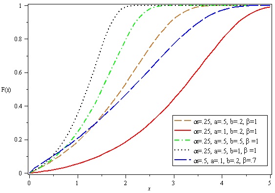
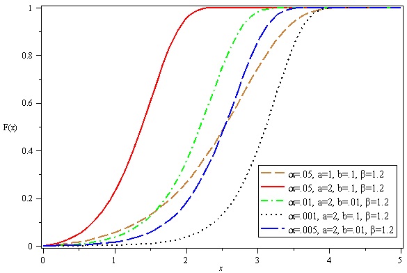
Figure 1: The CDF of various OGE-LFR distribution for different values of parameters.

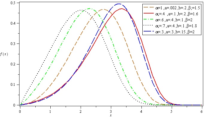
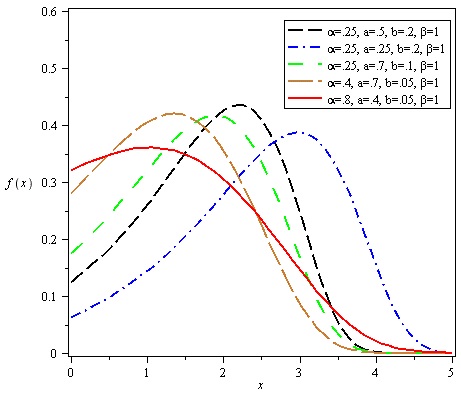
Figure 2: The PDF of various OGE-LFR distribution for different values of parameters.

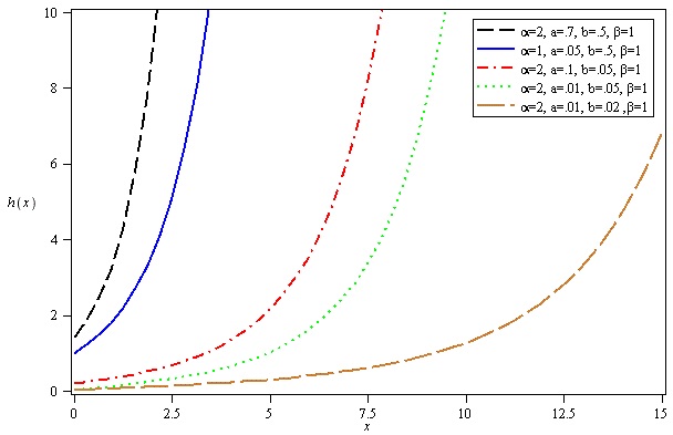
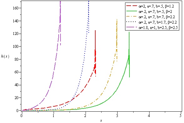
Figure 3: The Hazard function of various OGE-LFR distribution for different values of parameters.

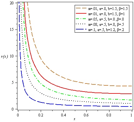
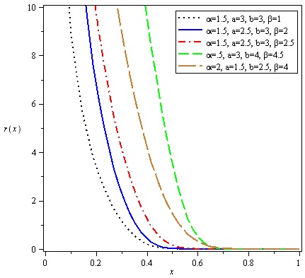
Figure 4: The Reversed hazard function of various OGE-LFR distribution for different values of parameters.

3 Statistical Properties

This section is devoted for studying some statistical properties for the odd generalized exponential-linear failure rate (OGE-LFR), specifically quantile function, median and the moments.

3.1 Quantile, Median and Mode

The quantile of the OGE-LFR($\Psi$) distribution is simply the solution of the following equation, with respect to $x_{q},\;0<q<1$

$$q=F(x_{q})=\left[1-e^{-\alpha\left(e^{ax_{q}+\frac{b}{2}x_{q}^{2}}-1\right)}\right]^{\beta}.$$ (3.1)

By solving equation (3.1), we obtain $x_{q}$ as follow

$$x_{q}=\frac{-a\pm\sqrt{a^{2}+2b\ln\left\{\ln\left[\frac{1}{\left(1-q^{\frac{1}{b}}\right)^{\frac{1}{\alpha}}}\right]\right\}}}{b}.$$

Since the quantile $x_{q}$ is positive, then we obtain the quantile as follow

$$x_{q}=\frac{-a+\sqrt{a^{2}+2b\ln\left\{\ln\left[\frac{1}{\left(1-q^{\frac{1}{b}}\right)^{\frac{1}{\alpha}}}\right]\right\}}}{b}.$$ (3.2)

The median can be derived from (3.2) be setting $q=\frac{1}{2}$. That is, the median is given by the following relation

$$Med=\frac{-a+\sqrt{a^{2}+2b\ln\left\{\ln\left[\frac{1}{\left(1-(\frac{1}{2})^{\frac{1}{b}}\right)^{\frac{1}{\alpha}}}\right]\right\}}}{b}.$$ (3.3)

Moreover, the mode of the OGE-LFR($\Psi$) distribution can be obtained by deriving its pdf with respect to $x$ and equal it to zero. Thus the mode of the OGE-LFR($\Psi$) distribution can be obtained as a nonnegative solution of the following nonlinear equation

$$1+b(a+bx)^{-2}-\alpha e^{ax+\frac{b}{2}x^{2}}\left[1-\frac{\beta-1}{e^{\alpha\left(e^{ax+\frac{b}{2}x^{2}}-1\right)}-1}\right]=0.$$ (3.4)

It is not possible to get an explicit solution of (3.4) in the general case. Numerical methods should be used such as fixed-point or bisection method to solve it.

3.2 The moments

In this subsection, we will derive the rth moments of the OGE-LFR($\Psi$) distribution as infinite series expansion.

Theorem 3.1.

The rth moment of a random variable $X\sim$OGE-LFR($\Psi$), where $\Psi=(\alpha,a,b,\beta)$ is given by

$$\mu_{r}^{\acute{}} = \sum^{\infty}_{i=0}\sum_{j=0}^{\infty}\sum^{j}_{k=0}\sum_{L=0}^{\infty}\tbinom{\beta-1}{i}\tbinom{j}{k}\left(-1\right)^{i+j+k}\frac{\beta\alpha^{j+1}b^{L}(i+1)^{j}}{j!L!2^{L}}\times$$

$$\left[\frac{(r+2L)!}{a^{r+2L}(j-k+1)^{r+2L+1}}+\frac{b(r+2L+1)!}{a^{r+2L+2}(j-k+1)^{r+2L+2}}\right].$$

Proof.

The rth moment of a random variable $X$ with pdf $f(x)$ is defined by

$$\mu_{r}^{{\acute{}}}=\int^{\infty}_{0}x^{r}f(x)dx.$$ (3.5)

Substituting from (2.2) into (3.5), we obtain

$$\mu_{r}^{{\acute{}}}=\int^{\infty}_{0}x^{r}\alpha\beta(a+bx)e^{ax+\frac{b}{2}x^{2}}e^{-\alpha\left(e^{ax+\frac{b}{2}x^{2}}-1\right)}\left[1-e^{-\alpha\left(e^{ax+\frac{b}{2}x^{2}}-1\right)}\right]^{\beta-1}dx.$$ (3.6)

Sinec $0<\left[1-e^{-\alpha\left(e^{ax+\frac{b}{2}x^{2}}-1\right)}\right]<1$ for $x>0,$ we obtain

$$\left[1-e^{-\alpha\left(e^{ax+\frac{b}{2}x^{2}}-1\right)}\right]^{\beta-1}=\sum_{i=0}^{\infty}\tbinom{\beta-1}{i}\left(-1\right)^{i}e^{-\alpha i\left(e^{ax+\frac{b}{2}x^{2}}-1\right)}.$$ (3.7)

Substituting from (3.7) into (3.6), we get

$$\mu_{r}^{{\acute{}}}=\sum_{i=0}^{\infty}\tbinom{\beta-1}{i}\left(-1\right)^{i}\alpha\beta\int^{\infty}_{0}x^{r}(a+bx)e^{ax+\frac{b}{2}x^{2}}e^{-\alpha(i+1)\left(e^{ax+\frac{b}{2}x^{2}}-1\right)}dx.$$

Using series expansion of $e^{-\alpha(i+1)\left(e^{ax+\frac{b}{2}x^{2}}-1\right)},$ we obtain

$$\mu_{r}^{{\acute{}}}=\sum_{i=0}^{\infty}\sum_{j=0}^{\infty}\tbinom{\beta-1}{i}\left(-1\right)^{i+j}\frac{\beta\alpha^{j+1}(i+1)^{j}}{j!}\int^{\infty}_{0}x^{r}(a+bx)e^{ax+\frac{b}{2}x^{2}}\left[e^{ax+\frac{b}{2}x^{2}}-1\right]^{j}dx.$$

Using binomial expansion of $\left[e^{ax+\frac{b}{2}x^{2}}-1\right]^{j},$ we obtain

$$\mu_{r}^{{\acute{}}} = \sum_{i=0}^{\infty}\sum_{j=0}^{\infty}\sum^{j}_{k=0}\tbinom{\beta-1}{i}\tbinom{j}{k}\left(-1\right)^{i+j+k}\frac{\beta\alpha^{j+1}(i+1)^{j}}{j!}\times$$

$$\hskip 76.82234pt\int^{\infty}_{0}x^{r}(a+bx)e^{a(j-k+1)x}\ e^{\frac{b}{2}(j-k+1)x^{2}}dx.$$

Using series expansion of $e^{\frac{b}{2}(j-k+1)x^{2}},$ we obtain

$$\left.\mu_{r}^{{\acute{}}}=\sum_{i=0}^{\infty}\sum_{j=0}^{\infty}\sum^{j}_{k=0}\sum_{L=0}^{\infty}\tbinom{\beta-1}{i}\tbinom{j}{k}\left(-1\right)^{i+j+k}\frac{\beta\alpha^{j+1}b^{L}(i+1)^{j}(j-k+1)^{L}}{j!L!2^{L}}\right.\times$$

$$\hskip 56.9055pt\left[a\int^{\infty}_{0}x^{r+2L}e^{a(i-k+1)x}dx+b\int^{\infty}_{0}x^{r+2L+1}\ e^{a(i-k+1)x}dx\right].$$

By using the definition of gamma function in the form, Zwillinger [14],

$$\Gamma(z)=x^{z}\int^{\infty}_{0}e^{tx}\ t^{z-1}dt,\;z,\;x>0.$$

Finally, we obtain the rth moment of OGE-LFR in the form

$$\mu_{r}^{{\acute{}}} = \sum_{i=0}^{\infty}\sum_{j=0}^{\infty}\sum^{j}_{k=0}\sum_{L=0}^{\infty}\tbinom{\beta-1}{i}\tbinom{j}{k}(-1)^{i+j+k}\frac{\beta\alpha^{j+1}b^{L}(i+1)^{j}(j-k+1)^{L}}{j!L!2^{L}}\times$$

$$\hskip 56.9055pt\left[\frac{(r+2L)!}{a^{r+2L}(j-k+1)^{r+2L+1}}+\frac{b(r+2L+1)!}{a^{r+2L+2}(j-k+1)^{r+2L+2}}\right].$$

This completes the proof. ∎

4 Order Statistics

Let X${}_{1:n},X_{2:n},\cdots,X_{n:n}$ denote the order statistics obtained from a random sample $X_{1},X_{2},\cdots,X_{n}$ which taken from a continuous population with cumulative distribution function (cdf) $F(x,\Psi)$ and probability density function (pdf) $f(x,\Psi)$, then the probability density function of $X_{r:n}$ is given by

$$f_{r:n}(x,\Psi)=\frac{1}{B(r,n-r+1)}\left[F(x,\Psi)\right]^{r-1}\left[1-F(x,\Psi)\right]^{n-r}f(x,\Psi),$$ (4.1)

where $f(x,\Psi),\ F(x,\Psi)$ are the pdf and cdf of OGE-LFR($\Psi$) distribution given by (LABEL:21) and (LABEL:22) respectively and $B(.,.)$ is the beta function, also we define first order statistics $X_{1:n}=\min(X_{1},X2,\cdots,X_{n})$, and the last order statistics as $X_{n:n}=\max(X_{1},X_{2},\cdots,X_{n})$. Since $0<F(x,\Psi)<1$ for $x>0$, we can use the binomial expansion of $\left[1-F(x,\Psi)\right]^{n-r}$ given as follows

$$\left[1-F(x,\Psi)\right]^{n-r}=\sum_{i=0}^{n-r}\binom{n-r}{i}(-1)^{i}\left[F(x,\Psi)\right]^{i}.$$ (4.2)

Substituting from (4.2) into (4.1), we obtain

$$f_{r:n}(x,\Psi)=\frac{1}{B(r,n-r+1)}f(x;\Psi)\sum_{i=0}^{n-r}\binom{n-r}{i}(-1)^{i}\left[F(x,\Psi)\right]^{i+r-1}.$$ (4.3)

Substituting from (2.1) and (2.2) into (4.3), we obtain

$$f_{r:n}(x;\alpha,a,b,\beta)=\sum_{i=0}^{n-r}\frac{(-1)^{i}n!}{i!(r-1)!(n-r-i)!(r+i)}f(\alpha,a,b,(r+i)\beta).$$ (4.4)

Relation (4.4) shows that $f_{r:n}(x,\Psi)$ is the weighted average of the odd generalized exponential-linear failure rate with different shape parameters.

5 Estimation and Inference

Now, we discuss the estimation of the OGE-LFR($\alpha,a,b,\beta$) parameters by using the method of maximum likelihood based on a complete sample.

5.1 Maximum likelihood estimators

Let $X_{1},X_{2},\cdots,X_{n}$ be a random sample of size n from $X\sim$ OGE-LFR($\alpha,a,b,\beta$) with observed values $x_{1},x_{2},\cdots,x_{n}$, then the log-likelihood function can be written as

$$\mathcal{L}=\prod^{n}_{i=1}f(x_{i};\alpha,a,b,\beta).$$ (5.1)

Substituting from (2.2) into (5.1), we get

$$\mathcal{L}=\prod^{n}_{i=1}\alpha\beta\left[a+bx_{i}\right]e^{ax_{i}+\frac{b}{2}x_{i}^{2}}e^{-\alpha\left[e^{ax_{i}+\frac{b}{2}x_{i}^{2}}-1\right]}\left[1-e^{-\alpha\left[e^{ax_{i}+\frac{b}{2}x_{i}^{2}}-1\right]}\right]^{\beta-1}.$$

The log-likelihood function can be written as

$$L = n\ln(\alpha)+n\ln(\beta)+\sum^{n}_{i=1}\ln\left[a+bx_{i}\right]+\sum^{n}_{i=1}\left[ax_{i}+\frac{b}{2}x_{i}^{2}\right]-$$ (5.2)

$$\alpha\sum^{n}_{i=1}\left[e^{ax_{i}+\frac{b}{2}x_{i}^{2}}-1\right]+(\beta-1)\sum^{n}_{i=1}\ln\left[1-e^{-\alpha\left(e^{ax_{i}+\frac{b}{2}x_{i}^{2}}-1\right)}\right].$$

The maximum likelihood estimates of the parameters are obtained by Differentiating the log-likelihood function L with respect to the parameters $\alpha,a,b$ and $\beta$ and setting the result to zero

$$\frac{\partial L}{\partial\beta} = \frac{n}{\beta}+\sum^{n}_{i=1}\ln\left[1-e^{-\alpha\left(e^{ax_{i}+\frac{b}{2}x_{i}^{2}}-1\right)}\right]=0,$$ (5.3)

$$\frac{\partial L}{\partial\alpha} = \frac{n}{\alpha}-\sum^{n}_{i=1}\left[\varphi(x_{i},a,b)-1\right]+(\beta-1)\sum^{n}_{i=1}\frac{\left[\varphi(x_{i},a,b)-1\right]}{\psi(x_{i},\alpha,a,b)}=0,$$ (5.4)

$$\frac{\partial L}{\partial a} = \sum^{n}_{i=1}\frac{1}{a+bx_{i}}+\sum^{n}_{i=1}x_{i}-\alpha\sum^{n}_{i=1}\varphi(x_{i},a,b)x_{i}+(\beta-1)\alpha\sum^{n}_{i=1}\frac{\varphi(x_{i},a,b)x_{i}}{\psi(x_{i},\alpha,a,b)}=0,$$

$$\frac{\partial L}{\partial b}=\sum^{n}_{i=1}\frac{x}{a+bx_{i}}+\frac{1}{2}\sum^{n}_{i=1}x_{i}^{2}-\frac{\alpha}{2}\sum^{n}_{i=1}\varphi(x_{i},a,b)x_{i}^{2}+\frac{(\beta-1)\alpha}{2}\sum^{n}_{i=1}\frac{\varphi(x_{i},a,b)x_{i}^{2}}{\psi(x_{i},\alpha,a,b)}=0,$$ (5.6)

Where the nonlinear functions $\psi(x_{i},\alpha,a,b)$ and $\varphi(x_{i},a,b)$ are given by

$$\varphi(x_{i},a,b) = e^{ax_{i}+\frac{b}{2}x_{i}^{2}},$$

$$\psi(x_{i},\alpha,a,b) = e^{\alpha\left[e^{ax_{i}+\frac{b}{2}x_{i}^{2}}-1\right]}-1.$$

From equation (5.3), we obtain the maximum likelihood estimate of $\beta$ in a closed form as follow

$$\hat{\beta}=\frac{-n}{\sum^{n}_{i=1}\ln\left[1-e^{-\alpha\left[e^{ax_{i}+\frac{b}{2}x_{i}^{2}}-1\right]}\right]}.$$ (5.7)

Substituting from (5.7) into (5.4), (5.1) and (5.6), we get the MLEs of $\alpha,a,b$ by solving the following system of non-linear equations

$$\frac{n}{\hat{\alpha}}-\sum^{n}_{i=1}\left[\varphi(x_{i},\hat{a},\hat{b})-1\right]+(\hat{\beta}-1)\sum^{n}_{i=1}\frac{\left[\varphi(x_{i},\hat{a},\hat{b})-1\right]}{\psi(x_{i},\hat{\alpha},\hat{a},\hat{b})} = 0,$$

$$\sum^{n}_{i=1}\frac{1}{\hat{a}+\hat{b}x_{i}}+\sum^{n}_{i=1}x_{i}-\hat{\alpha}\sum^{n}_{i=1}\varphi(x_{i},\hat{a},\hat{b})x_{i}+(\hat{\beta}-1)\hat{\alpha}\sum^{n}_{i=1}\frac{\varphi(x_{i},\hat{a},\hat{b})x_{i}}{\psi(x_{i},\hat{\alpha},\hat{a},\hat{b})} = 0,$$

$$\sum^{n}_{i=1}\frac{x}{\hat{a}+\hat{b}x_{i}}+\frac{1}{2}\sum^{n}_{i=1}x_{i}^{2}-\frac{\hat{\alpha}}{2}\sum^{n}_{i=1}\varphi(x_{i},\hat{a},\hat{b})x_{i}^{2}+\frac{(\hat{\beta}-1)\hat{\alpha}}{2}\sum^{n}_{i=1}\frac{\varphi(x_{i},\hat{a},\hat{b})x_{i}^{2}}{\psi(x_{i},\hat{\alpha},\hat{a},\hat{b})} = 0.$$

There is no closed form solution to these equations, so statistical software or numerical technique must be applied.

5.2 Asymptotic confidence bounds

In this subsection, we derive the asymptotic confidence intervals of the unknown parameters $\alpha,a,b$ and $\beta.$ As the sample size $n\longrightarrow\infty,$ then $(\hat{\alpha}-\alpha,\hat{a}-a,\hat{b}-b,\hat{\beta}-\beta)$ approaches a multivariate normal vector with zero means and the variance $I_{0}^{-1}(\hat{\alpha},\hat{a},\hat{b},\hat{\beta}),$ where $I_{0}^{-1}(\hat{\alpha},\hat{a},\hat{b},\hat{\beta})$ is the inverse of the observed information matrix which defined as follows

$$I_{0}^{-1} = -\left[\begin{array}[]{cccc}\frac{\partial^{2}}{\partial\alpha^{2}}&\frac{\partial^{2}}{\partial\alpha\partial a}&\frac{\partial^{2}}{\partial\alpha\partial b}&\frac{\partial^{2}}{\partial\alpha\partial\beta}\\ \frac{\partial^{2}}{\partial a\partial\alpha}&\frac{\partial^{2}}{\partial a^{2}}&\frac{\partial^{2}}{\partial a\partial b}&\frac{\partial^{2}}{\partial a\partial\beta}\\ \frac{\partial^{2}}{\partial b\partial\alpha}&\frac{\partial^{2}}{\partial b\partial a}&\frac{\partial^{2}}{\partial b^{2}}&\frac{\partial^{2}}{\partial b\partial\beta}\\ \frac{\partial^{2}}{\partial\beta\partial\alpha}&\frac{\partial^{2}}{\partial\beta\partial a}&\frac{\partial^{2}}{\partial\beta\partial b}&\frac{\partial^{2}}{\partial\beta^{2}}\end{array}\right]^{-1}$$ (5.12)

$$= \left[\begin{array}[]{cccc}Var(\hat{\alpha})&cov(\hat{\alpha},\hat{a})&cov(\hat{\alpha},\hat{b})&cov(\hat{\alpha},\hat{\beta})\\ cov(\hat{a},\hat{\alpha})&Var(\hat{a})&cov(\hat{a},\hat{b})&cov(\hat{a},\hat{\beta})\\ cov(\hat{b},\hat{\alpha})&cov(\hat{b},\hat{a})&Var(\hat{b})&cov(\hat{b},\hat{\beta})\\ cov(\hat{\beta},\hat{\alpha})&cov(\hat{\beta},\hat{a})&cov(\hat{\beta},\hat{b})&Var(\hat{\beta})\end{array}\right].$$ (5.17)

The second partial derivatives included in $I_{0}^{-1}$ are given as follows

$$\frac{\partial^{2}L}{\partial\beta^{2}} = \frac{-n}{\beta^{2}},\hskip 102.43008pt\frac{\partial^{2}L}{\partial\beta\partial\alpha}=\sum^{n}_{i=1}\frac{\varphi(x_{i},a,b)-1}{\psi(x_{i},\alpha,a,b)},$$

$$\frac{\partial^{2}L}{\partial\beta\partial a} = \alpha\sum^{n}_{i=1}\frac{x_{i}\varphi(x_{i},a,b)}{\psi(x_{i},\alpha,a,b)},\hskip 42.67912pt\frac{\partial^{2}L}{\partial\beta\partial b}=\frac{\alpha}{2}\sum^{n}_{i=1}\frac{x_{i}^{2}\varphi(x_{i},a,b)}{\psi(x_{i},\alpha,a,b)},$$

$$\frac{\partial^{2}L}{\partial\alpha^{2}} = \frac{-n}{\alpha^{2}}-(\beta-1)\sum^{n}_{i=1}\frac{\left[\varphi(x_{i},a,b)-1\right]^{2}\left[\psi(x_{i},\alpha,a,b)+1\right]}{\left[\psi(x_{i},\alpha,a,b)\right]^{2}},$$

$$\frac{\partial^{2}L}{\partial\alpha\partial a} = -\sum^{n}_{i=1}x_{i}\varphi(x_{i},a,b)+(\beta-1)\sum^{n}_{i=1}\frac{x_{i}\varphi(x_{i},a,b)h(x_{i},\alpha,a,b)}{\left[\psi(x_{i},\alpha,a,b)\right]^{2}},$$

$$\frac{\partial^{2}L}{\partial\alpha\partial b} = -\frac{1}{2}\sum^{n}_{i=1}x_{i}^{2}\varphi(x_{i},a,b)+\frac{(\beta-1)}{2}\sum^{n}_{i=1}\frac{x_{i}^{2}\varphi(x_{i},a,b)h(x_{i},\alpha,a,b)}{\left[\psi(x_{i},\alpha,a,b)\right]^{2}},$$

$$\frac{\partial^{2}L}{\partial a^{2}} = -\sum^{n}_{i=1}\frac{1}{\left(a+bx_{i}\right)^{2}}-\alpha\sum^{n}_{i=1}x_{i}^{2}\varphi(x_{i},a,b)+(\beta-1)\alpha\times$$

$$\hskip 85.35826pt\sum^{n}_{i=1}\frac{x_{i}^{2}\varphi(x_{i},a,b)\tau(x_{i},\alpha,a,b)}{\left[\psi(x_{i},\alpha,a,b)\right]^{2}},$$

$$\frac{\partial^{2}L}{\partial a\partial b} = -\sum^{n}_{i=1}\frac{x_{i}}{\left(a+bx_{i}\right)^{2}}-\frac{\alpha}{2}\sum^{n}_{i=1}x_{i}^{3}\varphi(x_{i},a,b)+\frac{(\beta-1)\alpha}{2}\times$$

$$\hskip 85.35826pt\sum^{n}_{i=1}\frac{x_{i}^{3}\varphi(x_{i},a,b)\tau(x_{i},\alpha,a,b)}{\left[\psi(x_{i},\alpha,a,b)\right]^{2}},$$

$$\frac{\partial^{2}L}{\partial b^{2}} = -\sum^{n}_{i=1}\frac{x_{i}^{2}}{\left(a+bx_{i}\right)^{2}}-\frac{\alpha}{4}\sum^{n}_{i=1}x_{i}^{4}\varphi(x_{i},a,b)+\frac{(\beta-1)\alpha}{4}$$

$$\hskip 85.35826pt\sum^{n}_{i=1}\frac{x_{i}^{4}\varphi(x_{i},a,b)\tau(x_{i},\alpha,a,b)}{\left[\psi(x_{i},\alpha,a,b)\right]^{2}},$$

where the nonlinear functions $\psi(x_{i},\alpha,a,b),$ $\varphi(x_{i},a,b),$ $h(x_{i},\alpha,a,b)$ and $\tau(x_{i},\alpha,a,b)$ are given by

$$\varphi(x_{i},a,b)=e^{ax_{i}+\frac{b}{2}x_{i}^{2}},\qquad\psi(x_{i},\alpha,a,b)=e^{\alpha\left(e^{ax_{i}+\frac{b}{2}x_{i}^{2}}-1\right)}-1,$$

$$h(x_{i},\alpha,a,b)=e^{\alpha\left(e^{ax_{i}+\frac{b}{2}x_{i}^{2}}-1\right)}\left[1-\alpha\left(e^{ax_{i}+\frac{b}{2}x_{i}^{2}}-1\right)\right]-1,$$

$$\tau(x_{i},\alpha,a,b)=e^{\alpha\left(e^{ax_{i}+\frac{b}{2}x_{i}^{2}}-1\right)}\left[1-\alpha e^{ax_{i}+\frac{b}{2}x_{i}^{2}}\right]-1.$$

The above approach is used to derive the $(1-\delta)100\%$ confidence intervals for the parameters $\alpha,a,b$ and $\beta$ as in the following forms

$$\hat{\alpha}\pm Z_{\frac{\delta}{2}}\sqrt{Var(\hat{\alpha})},\;\hat{a}\pm Z_{\frac{\delta}{2}}\sqrt{Var(\hat{a})},\;\hat{b}\pm Z_{\frac{\delta}{2}}\sqrt{Var(\hat{b})},\;\hat{\beta}\pm Z_{\frac{\delta}{2}}\sqrt{Var(\hat{\beta})},$$

where $Z_{\frac{\delta}{2}}$ is the upper ($\frac{\delta}{2}$)th percentile of the standard normal distribution.

6 Data Analysis

Now we use a real data set to show that the OGE-LFR distribution can be a better model, comparing with many known distributions such as the Exponential(E), Generalized Exponential(GE), Linear Failure Rate(LFR), New Generalized Linear Exponential (NGLE) and Transmuted Linear Exponential (TLE). Consider the data have been obtained from Aarset [1], and widely reported in many literatures. It represents the lifetimes of 50 devices, and also, possess a bathtub-shaped failure rate property, Table 1.

Table 1: The data from Aarset [1].

0.1	0.2	1	1	1	1	1	2	3	6	7	11	12	18
18	18	18	18	21	32	36	40	45	46	47	50	55	60
63	63	67	67	67	67	72	75	79	82	82	83	84	84
84	85	85	85	85	85	86	86

The MLEs of the unknown parameters and the corresponding Kolmogorov–Smirnov(K–S) test statistic for the six models are given in Table 2.

Table 2: The MLES of the parameters, the K–S values and p-values.

The model	MLE of the parameters	K–S	P-value(K-S)
E	$\hat{\alpha}$ = 0.0219	0.1911	0.0519
GE	$\hat{\alpha}$ = 0.0212, $\hat{\beta}$ = 0.9012	0.1940	0.0514
LFR	$\hat{a}$ = 0.014, $\hat{b}$ = 2.4$\times 10^{-4}$	0.1955	0.0370
NGLE	$\hat{a}$ = 0.0012, $\hat{b}$ = 0.0127, $\hat{c}$ =1.0682, $\hat{\beta}$ = 0.7231	0.2030	0.0276
TLE	$\hat{a}$ = 0.0145, $\hat{b}$ = 2.4186 $\times 10^{-4},$ $\hat{\lambda}$ = -0.0948	0.1740	0.0855
OGE-LFR	$\hat{\alpha}$ = 472.404, $\hat{a}$ = 8.218 $\times 10^{-6}$, $\hat{b}$ = 6.427 $\times 10^{-7},$ $\hat{\beta}$ = 0.529	0.1627	0.12830

The values of the log-likelihood functions (-L), AIC (Akaike Information Criterion), the statistics AICC (Akaike Information Citerion with correction), BIC (Bayesian Information Criterion) and HQIC (Hannan-Quinn information criterion) are calculated in Table 3 for the six distributions in order to verify which distribution fits better to these data.

Table 3: The –L, AIC, AICC, BIC and HQIC for devices data.

The model	–L	AIC	AICC	BIC	HQAIC
E	241.090	484.1792	484.2625	486.0912	484.908
GE	240.3855	484.7710	485.0264	488.5951	486.227
LFR	238.064	480.128	480.383	483.952	481.584
NGLE	239.49	486.98	487.869	494.6281	489.892
TLE	238.01	482.02	482.54	487.756	484.204
OGE-LFR	232.865	473.730	474.618	481.378	476.642

Based on Tables 2 and 3, it is shown that OGE-LFR($\alpha,a,b,\beta$) model provide better fit to the data rather than other distributions which we compared with because it has the smallest value of (K-S), AIC, AICC, BIC and HQIC test.

To show that the likelihood equation have unique solution, we plot the profiles of the log-likelihood function of $\alpha,a,b$ and $\beta$ in Figures 5-6.

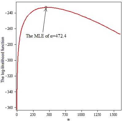
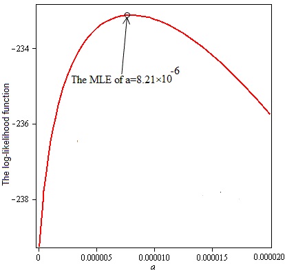
Figure 5: The profile of the log-likelihood function of $\alpha,a$.

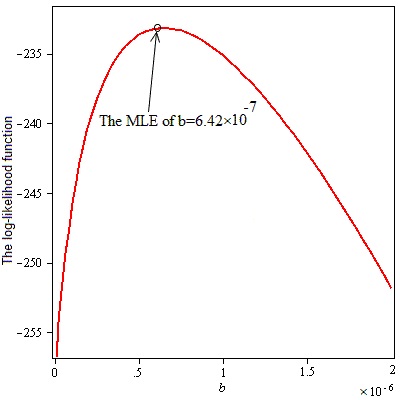
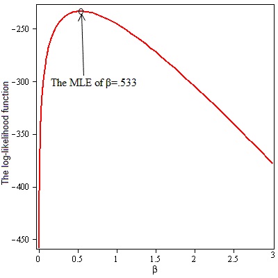
Figure 6: The profile of the log-likelihood function of $b,\beta$.

The nonparametric estimate of the survival function using the Kaplan-Meier method and its fitted parametric estimations when the distributions is assumed to be E, GE, LFR, NGLE, TLE and OGE-LFR are computed and plotted in Figure 7.

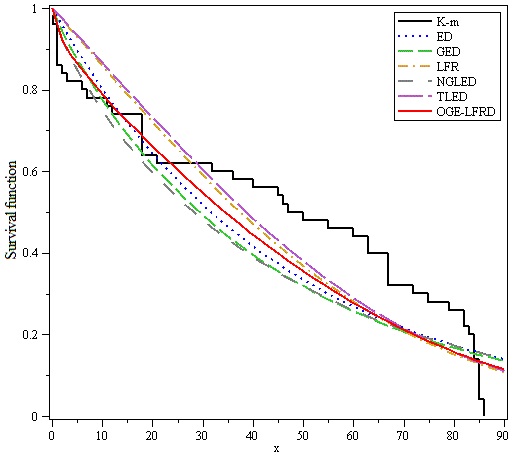
Figure 7: The Kaplan-Meier estimate of survival function and fitted survival functions.

Figures 8 and 9, give the form of the probability density functions and the hazard functions for the ED, GED, LFRD, NGLED, TLED, OGE-LFRD distributions which are used to fit the data after replacing the unknown parameters included in each distribution by their MLE.

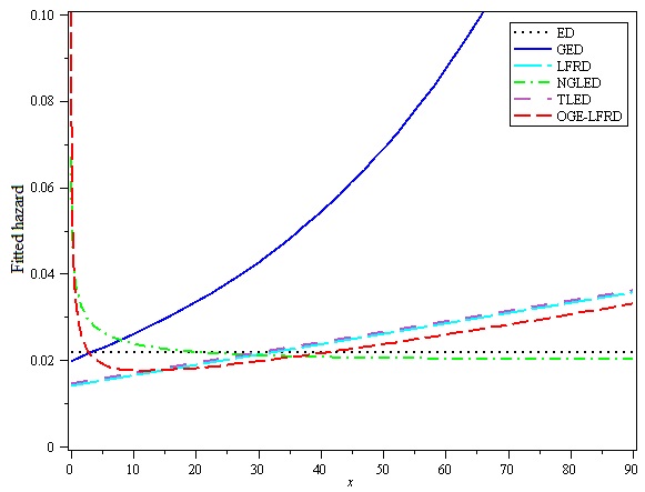
Figure 8: The Fitted hazard functions for the data.

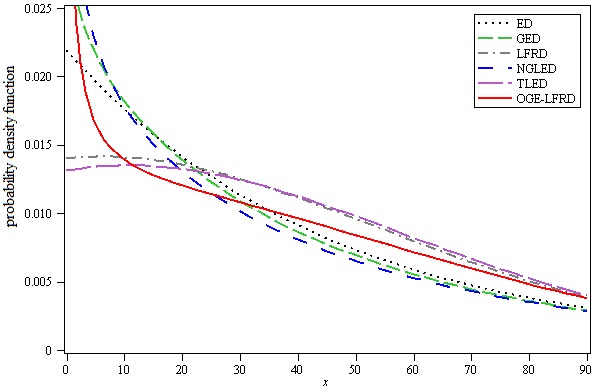
Figure 9: The Fitted probability density functions for the data.

7 Conclusions

In this article, we have introduced a new four-parameter model called odd generalized exponential linear failure rate distribution. We refer to the new model as the OGE-LFR distribution and study some of its mathematical and statistical properties. We provide the pdf, the cdf, the hazard rate function and the reversed hazard function for the new model also we provide an explicit expression for the moments. The model parameters are estimated by maximum likelihood method. We use application on set of real data to compare the OGE-LFR with other known distributions such as Exponential (E), Generalized Exponential (GE), Linear Failure Rate (LFR), New Generalized Linear Exponential (NGLE) and Transmuted Linear Exponential (TLE). Applications on set of real data showed that the OGE-LFR is the best distribution for fitting these data sets compared with ED, GED, LFRD, NGLED and TLED distributions.

References

- [1] Aarset, M. V. (1987). How to identify a bathtub hazard rate. IEEE Transactions on Reliability 36(1), 106–108.
- [2] Bain, L. J. (1974). Analysis for the linear failure-rate life-testing distribution. Technometrics, 16(4), 551–559.
- [3] El-Damcese, M. A., Mustafa, A., El-Desouky, B. S., & Mustafa, M. E. (2015). The odd generalized exponential gompertz. arXiv preprint arXiv:1507.06400.
- [4] Gupta, R. D., & Kundu, D. (2007). Generalized exponential distribution: Existing results and some recent developments. Journal of Statistical Planning and Inference, 137(11), 3537–3547.
- [5] Gupta, R. D., & Kundu, D. (1999). Theory & methods: Generalized exponential distributions. Australian & New Zealand Journal of Statistics, 41(2), 173–188.
- [6] Jamkhaneh, E. (2014). Modified generalized linear failure rate distribution: Properties and reliability analysis. International Journal of Industrial Engineering Computations, 5(3), 375–386.
- [7] Jafari, A. A., & Mahmoudi, E. (2012). Beta-linear failure rate distribution and its applications. arXiv preprint arXiv:1212.5615.
- [8] Mudholkar, G. S., Srivastava, D. K., & Freimer, M. (1995). The exponentiated Weibull family: a reanalysis of the bus-motor-failure data. Technometrics, 37(4), 436–445.
- [9] Mahmoud, M. A. W., & Alam, F. M. A. (2010). The generalized linear exponential distribution. Statistics & probability letters, 80(11), 1005–1014.
- [10] Sarhan, A. M., & Kundu, D. (2009). Generalized linear failure rate distribution. Communications in Statistics – Theory and Methods, 38(5), 642–660.
- [11] Tian, Y. Z., Tian, M. Z., & Zhu, Q. Q. (2014). A new generalized linear exponential distribution and its applications. Acta Mathematicae Applicatae Sinica, English Series, 30(4), 1049–1062.
- [12] Tian, Y., Tian, M., & Zhu, Q. (2014). Transmuted linear exponential distribution: A new generalization of the linear exponential distribution. Communications in Statistics-Simulation and Computation, 43(10), 2661–2677.
- [13] Tahir, M. H., Cordeiro, G. M., Alizadeh, M., Mansoor, M., Zubair, M., & Hamedani, G. G. (2015). The odd generalized exponential family of distributions with applications. Journal of Statistical Distributions and Applications, 2(1), 1–28.
- [14] Zwillinger, D. (2014). Table of integrals, series, and products. Elsevier.