EFFECTIVE PROPERTIES OF PERIODIC TUBULAR STRUCTURES

Abstract

A method is described to calculate effective tensor properties of a periodic array of two-phase dielectric tubes embedded in a host matrix. The method uses Weierstrass’ quasiperodic functions for representation of the potential that considerably facilitates the problem and allows us to find an exact expression for the effective tensor. For weakly interacting tubes we obtain Maxwell-like approximation of the effective parameter which is in very good agreement with experimental results in considered examples.

1 Introduction

The problem of evaluating the effective properties (permittivity, conductivity, etc.) of periodic heterogeneous materials has been extensively investigated. Its solution for noninteracting particles was suggested by Maxwell [17], which has become ubiquitous in physics and engineering as well as an indispensable benchmark asymptotics. Despite apparent limitations, it provides a good approximation in a certain range of parameters for the estimation of optical properties of square lattice of carbon nanotubes [8],[26] as well as optical properties of artificially engineered microstructured materials [16].

The seminal paper of Rayleigh [25] predestined the development in this area for many decades to come. It contained the ideas of the multipole expansion method, relation of the potential with the elliptic functions, its application to elasticity and wave propagation. Rayleigh’s method was extended to a regular arrays of cylinders [24],[18],[23] as well as to the dynamic problems [28].

Application of Rayleigh’s approach to arbitrary lattices, however, encounters two obstacles. The distribution of stream lines is not known for the medium whose effective properties are described by a tensor. As a result, the method used in [25] for evaluation of a scalar is not applicable for determination of the effective tensor. Next, the method entails conditionally convergent sum whose summation order is obscure. That hampers further development of the method.

The advantages of application of the elliptic and meromorphic functions to the problems of determination of the effective properties of perforated plates and shells had been clearly demonstrated in [13]. Elliptic functions were successfully employed for a rectangular lattice of circular inclusions [1] as well as in the problem of periodic fibrous composites in applications to biological tissues [6]. A method of functional equations [22], [27] employing analytic functions was used to find an expression of the permittivity tensor for small volume fraction of inclusions.

Another method was introduced in [2, 3, 4, 5] and is based on the study of the analytic properties of the effective parameters. This approach was extended in [19, 20, 21] and proved to be efficient for obtaining bounds on complex effective parameters. Its mathematical justification is given in [11, 12].

In this paper we represent the potential in terms of Weierstrass’ $\zeta$-functions and their derivatives (an analog of periodically distributed multipoles). This ensures periodicity of the electric field in the whole plane and avoids the problem of summation of conditionally convergent series. Then we determine the average electric field and electric displacement within the parallelogram of the periods. It allows us to find an explicit formula for the tensor of effective properties.

2 Representation of solution and compliance with the boundary conditions

We consider an infinite periodic array of parallel tubes with the periods $2\bm{\tau}_{1}$ and $2\bm{\tau}_{2}$ (see Figure 1) embedded in a homogeneous medium with dielectric constant $\varepsilon_{ex}$. Dielectric constant of the tubes of inner radii $b$ and outer radii $a$ is denoted by $\varepsilon_{tu}$. We also suppose that the tubes are filled with a material with dielectric constant $\varepsilon_{in}$. A homogeneous electric field $\bm{E}$ is applied in the direction perpendicular to the axes of the tubes. In the plane of complex variable $z=x+iy$ we introduce the electric potential $u(z)$ which satisfies the equation

$$\nabla\cdot\left[\varepsilon\nabla u\right]=0,\quad\varepsilon=\left\{\begin{array}[]{l}\varepsilon_{in},\quad 0\leqslant r<b,\\[5.69054pt] \varepsilon_{tu},\quad b<r<a,\\[5.69054pt] \varepsilon_{ex},\quad r>a.\end{array}\right.$$ (4)

On the boundaries $r=a$ and $r=b$ of the tubes we impose continuity conditions

$$\left\llbracket u\right\rrbracket=0,$$ (5)

$$\left\llbracket\varepsilon\,\frac{\partial u}{\partial n}\right\rrbracket=0,$$ (6)

where brackets $\llbracket\cdot\rrbracket$ denote the jump of the enclosed quantity across the interface. In addition, we require the field $\nabla u$ to be periodic

$$\nabla u(z+2\tau_{i})=\nabla u(z),\quad i=1,2,$$ (7)

and normalized in such a way that when the radius of the tubes approaches zero the field tends to the homogeneous one of intensity $E=E_{x}-iE_{y}$

$$u_{ex}(z)\to-Ez\quad\text{as}\quad a\to 0.$$ (8)

Figure 1: (a) A fragment of an infinite periodic array of tubes with the periods $2\bm{\tau}_{1}$ and $2\bm{\tau}_{2}$ and a fundamental period parallelogram $ABCD$. (b) Material and geometric parameters of the tubes.

Following [10], we represent complex potential $u(z)$ in the form

$$u_{in}(z) =Ea\sum_{n=0}^{\infty}\left[A_{n}\left(\frac{z}{b}\right)^{2n+1}+B_{n}\left(\frac{\bar{z}}{b}\right)^{2n+1}\right],$$ (9)

$$u_{tu}(z) =Ea\sum_{n=0}^{\infty}\left[C_{n}\left(\frac{z}{b}\right)^{2n+1}+D_{n}\left(\frac{\bar{z}}{b}\right)^{2n+1}+E_{n}\left(\frac{a}{z}\right)^{2n+1}+F_{n}\left(\frac{a}{\bar{z}}\right)^{2n+1}\right],$$ (10)

$$u_{ex}(z) =-Ez+Ea\sum_{n=0}^{\infty}\frac{a^{2n+1}}{(2n)!}\left[G_{n}\zeta^{(2n)}(z)+H_{n}\zeta^{(2n)}(\bar{z})\right],$$ (11)

where $A_{n},\ldots,H_{n}$ are unknown complex dimensionless coefficients, $\bar{z}$ stands for the complex conjugation, and $\zeta^{(2n)}(z)$ is $2n$-th derivative of the Weierstrass $\zeta$-function [15]

$$\zeta(z)=\frac{1}{z}+{\sum_{m,n}}^{\prime}\left[\frac{1}{z-P_{m,n}}+\frac{1}{P_{m,n}}+\frac{z}{P_{m,n}^{\,2}}\right].$$ (12)

Here $P_{m,n}=2m\tau_{1}+2n\tau_{2}$. Prime in the sum means that summation is extended over all pairs $m,\,n$ except $m=n=0$. Since the electric field $E$ is periodic, the potential $u(z)$ should be represented as the sum of periodic and linear functions. The Weierstrass $\zeta$-function has just that property [7]

$$\zeta(z+2\tau_{k})=\zeta(z)+2\eta_{k},\quad\eta_{k}=\zeta(\tau_{k}),\quad k=1,2,$$ (13)

where constants $\eta_{1}$ and $\eta_{2}$ are related by the Legendre identity

$$\eta_{1}\tau_{2}-\eta_{2}\tau_{1}=\frac{\pi i}{2}.$$ (14)

Its derivatives however are periodic functions, so that condition (7) is fulfilled. Also, from (12) it follows that

$$\oint_{ABCD}\zeta^{(n)}(z)\,dz=0,\quad n\geqslant 1.$$ (15)

To satisfy conditions (5)-(6) on the boundary $r=a$ we expand $\zeta(z)$ and its even derivatives in a Laurent series

$$\zeta^{(2n)}(z) =\frac{(2n)!}{z^{2n+1}}-\sum_{k=0}^{\infty}s_{n+k+1}\,\frac{(2n+2k+1)!}{(2k+1)!}\,z^{2k+1},\quad n\geqslant 0,\quad s_{1}=0,$$ (16)

where

$$s_{k}={\sum_{n,m}}^{\prime}\frac{1}{P_{m,n}^{\,2k}},\quad k=2,3,\ldots.$$ (17)

Due to the symmetry of the lattice the only nonzero sums (17) are those with even powers of $P_{m,n}$.

Compliance with the boundary conditions (5)-(6) leads to an infinite system of linear equations

$$H_{n} -\gamma_{n}\sum_{k=0}^{\infty}s_{n+k+1}\frac{(2n+2k+1)!}{(2k)!(2n+1)!}\,G_{k}\,a^{2n+2k+2}=\gamma_{n}\delta_{n,0},$$ (18)

$$G_{n} -\gamma_{n}\sum_{k=0}^{\infty}s_{n+k+1}\frac{(2n+2k+1)!}{(2k)!(2n+1)!}\,H_{k}\,a^{2n+2k+2}=0,$$ (19)

where

$$\gamma_{n} =\frac{\alpha-\widetilde{\alpha}\nu^{4n+2}}{1-\alpha\widetilde{\alpha}\nu^{4n+2}},$$ (20)

$$\alpha =\frac{\varepsilon_{tu}-\varepsilon_{ex}}{\varepsilon_{tu}+\varepsilon_{ex}},$$ (21)

$$\widetilde{\alpha} =\frac{\varepsilon_{tu}-\varepsilon_{in}}{\varepsilon_{tu}+\varepsilon_{in}},$$ (22)

$$\nu =\frac{b}{a},\quad 0\leqslant\nu<1,$$ (23)

and $\delta_{n,0}$ is the Kronecker delta. The other coefficients are expressed through $H_{n}$ and $G_{n}$ as follows:

$$A_{n} =\frac{(\alpha-1)(1+\widetilde{\alpha})\nu^{2n+1}}{\alpha-\widetilde{\alpha}\nu^{4n+2}}\,H_{n}, \quad B_{n} =\frac{(\alpha-1)(1+\widetilde{\alpha})\nu^{2n+1}}{\alpha-\widetilde{\alpha}\nu^{4n+2}}\,G_{n},$$ (24)

$$C_{n} =\frac{(\alpha-1)\nu^{2n+1}}{\alpha-\widetilde{\alpha}\nu^{4n+2}}\,H_{n}, \quad D_{n} =\frac{(\alpha-1)\nu^{2n+1}}{\alpha-\widetilde{\alpha}\nu^{4n+2}}\,G_{n},$$ (25)

$$F_{n} =\frac{\widetilde{\alpha}(\alpha-1)\nu^{4n+2}}{\alpha-\widetilde{\alpha}\nu^{4n+2}}\,H_{n}, \quad E_{n} =\frac{\widetilde{\alpha}(\alpha-1)\nu^{4n+2}}{\alpha-\widetilde{\alpha}\nu^{4n+2}}\,G_{n}.$$ (26)

We introduce new variables

$$x_{n} =H_{n}+G_{n},$$ (27)

$$y_{n} =H_{n}-G_{n}.$$ (28)

Then equations (18)-(19) become independent

$$x_{n} -\gamma_{n}\sum_{k=0}^{\infty}s_{n+k+1}\frac{(2n+2k+1)!}{(2k)!(2n+1)!}\,x_{k}\,a^{2n+2k+2}=\gamma_{0}\delta_{n,0},$$ (29)

$$y_{n} +\gamma_{n}\sum_{k=0}^{\infty}s_{n+k+1}\frac{(2n+2k+1)!}{(2k)!(2n+1)!}\,y_{k}\,a^{2n+2k+2}=\gamma_{0}\delta_{n,0}.$$ (30)

We will analyze (29)-(30) by the approach described in [10]. First, we introduce parameter $h$

$$h=\frac{a}{\ell},\quad h\leqslant\frac{1}{2},$$ (31)

where $\ell$ is the least distance between the centers of the tubes

$$\ell=\min(2|\tau_{1}|,2|\tau_{2}|,2|\tau_{1}-\tau_{2}|).$$ (32)

Then we denote by $S_{k}$ the dimensionless lattice sums

$$S_{k} ={\sum_{n,m}}^{\prime}\left(\frac{\ell}{P_{m,n}}\right)^{2k},\;k=2,3,\ldots,\;S_{1}=0,$$ (33)

and represent both equations (29)-(30) as

$${\bm{u}}-\mathcal{G}(h){\bm{u}}={\bm{v}},$$ (34)

where ${\bm{u}}=(u_{0},u_{1},\ldots)\in\ell_{\infty}(\mathbb{C})$, ${{\bm{v}}}=\gamma_{0}\,\delta_{n,0}$, and operator $\mathcal{G}(h)$ is defined by

$$\left(\mathcal{G}(h)\,{\bm{u}}\right)_{n}=\gamma_{n}\sum_{k=0}^{\infty}G_{n,k}\,u_{k}\,h^{2n+2k+2},$$ (35)

where

$$G_{n,k} =\pm\frac{(2n+2k+1)!}{(2k)!(2n+1)!}\,S_{n+k+1},\quad G_{0,0}=0.$$ (36)

Properties of equation (34) describes the following

Theorem 1.

Equation (34) has the following properties:

1. For each $0\leqslant h\leqslant\frac{1}{2}$ $\mathcal{G}(h)$ is a bounded operator in $l_{\infty}({\mathbb{C}})$.

2. If $0\leqslant h<\frac{1}{2}$ then operator $\mathcal{G}(h)$ is compact.

3. The norm of $\mathcal{G}(h)$ is estimated by

   $$\|\mathcal{G}(h)\|_{\infty}\leqslant\left|\gamma_{0}\right|\,\left(\left(\frac{h}{1-h}\right)^{2}+\left(\frac{h}{1+h}\right)^{2}\right)\sup_{n}|S_{n}|.$$ (37)

4. If $\|\mathcal{G}(h)\|_{\infty}<1$ then (34) has a unique solution ${{\bm{u}}}_{0}\in c_{0}(\mathbb{C})$. Truncated solution of (34) converges exponentially to ${{\bm{u}}}_{0}$ and can be represented as a convergent power series in $h$.

Proof of the theorem is almost identical to that given in [9].

We will seek for the series solution of (34) in the form

$$u_{n}=\gamma_{0}\,\delta_{n,0}+\sum_{m=0}^{\infty}p_{n,m}h^{2n+2m+2}.$$ (38)

Substitution of (38) into (34) gives a recurrence relation for the coefficients $p_{n,m}$:

$$p_{n,0} =\gamma_{0}\,G_{n,0},$$ (39)

$$p_{n,k} =\sum_{m=0}^{\left[\frac{k-1}{2}\right]}G_{n,m}\,p_{m,k-2m-1},$$ (40)

where $[\nu]$ denotes the integral part of $\nu$.

In the next section it will be shown that the effective properties are determined by only $x_{0}$ and $y_{0}$ in (29)-(30) which we denote as

$$x_{0} =\gamma_{0}\lambda,\quad y_{0}=\gamma_{0}\mu.$$ (41)

From (39)-(40) one can find the series expansion for $\mu$ and $\lambda$. The first few terms of their expansion are given by

$$\lambda =1+3\gamma_{0}\gamma_{1}S_{2}^{2}h^{8}+5\gamma_{0}\gamma_{2}S_{3}^{2}h^{12}+30\gamma_{0}\gamma_{1}^{2}S_{2}^{2}S_{3}h^{14}$$

$$+\left(9\gamma_{0}^{2}\gamma_{1}^{2}S_{2}^{4}+7\gamma_{0}\gamma_{3}S_{4}^{2}\right)h^{16}+210\gamma_{0}\gamma_{1}\gamma_{2}S_{2}S_{3}S_{4}h^{18}$$

$$+\left(15\gamma_{1}S_{2}^{2}\left(\gamma_{0}^{2}\gamma_{2}S_{3}^{2}+20\gamma_{0}\gamma_{1}^{2}S_{3}^{2}\right)+15\gamma_{0}^{2}\gamma_{1}\gamma_{2}S_{2}^{2}S_{3}^{2}+9\gamma_{0}\gamma_{4}S_{5}^{2}\right)h^{20}+O\left(h^{22}\right),$$ (42)

$$\mu =1+3\gamma_{0}\gamma_{1}S_{2}^{2}h^{8}+5\gamma_{0}\gamma_{2}S_{3}^{2}h^{12}-30\gamma_{0}\gamma_{1}^{2}S_{2}^{2}S_{3}h^{14}$$

$$+\left(9\gamma_{0}^{2}\gamma_{1}^{2}S_{2}^{4}+7\gamma_{0}\gamma_{3}S_{4}^{2}\right)h^{16}-210\gamma_{0}\gamma_{1}\gamma_{2}S_{2}S_{3}S_{4}h^{18}$$

$$+\left(15\gamma_{1}S_{2}^{2}\left(\gamma_{0}^{2}\gamma_{2}S_{3}^{2}+20\gamma_{0}\gamma_{1}^{2}S_{3}^{2}\right)+15\gamma_{0}^{2}\gamma_{1}\gamma_{2}S_{2}^{2}S_{3}^{2}+9\gamma_{0}\gamma_{4}S_{5}^{2}\right)h^{20}+O\left(h^{22}\right).$$ (43)

3 Determination of the effective permittivity tensor

Effective permittivity tensor ${\bm{\varepsilon}}^{\ast}$ relates the average electric displacement $\langle{\bm{D}}\rangle$ and the average electric field $\langle\bm{E}\rangle$

$$\langle{\bm{D}}\rangle={\bm{\varepsilon}}^{\ast}\langle{\bm{E}}\rangle.$$ (1)

Observe that

$$\langle{\bm{E}}\rangle =\frac{1}{S}\iint_{S}\bm{E}\,dS=\frac{1}{S}\iint_{S_{in}}\bm{E}_{in}\,dS+\frac{1}{S}\iint_{S_{tu}}\bm{E}_{tu}\,dS+\frac{1}{S}\iint_{S_{ex}}\bm{E}_{ex}\,dS,$$ (2)

while

$$\langle{\bm{D}}\rangle =\frac{1}{S}\iint_{S}\bm{D}\,dS=\frac{\varepsilon_{in}}{S}\iint_{S_{in}}\bm{E}_{in}\,dS+\frac{\varepsilon_{tu}}{S}\iint_{S_{tu}}\bm{E}_{tu}\,dS+\frac{\varepsilon_{ex}}{S}\iint_{S_{ex}}\bm{E}_{ex}\,dS,$$ (3)

where $S$ is the total area of the parallelogram $ABCD$, $S_{in}$ is the disk of radius $b$, $S_{tu}$ is the annular domain with $b\leqslant r\leqslant a$, and $S_{ex}$ is the part of the parallelogram outside the disk $r\leqslant a$. Thus, in (2)-(3) we need to evaluate three distinct integrals.

Using the mean-value property of harmonic functions in the first integral and relations (24), (27)-(28) we get

$$\iint_{S_{in}}\bm{E}_{in}\,dS =\bm{E}_{in}(0,0)S_{in}=-E\,ab\left(A_{0}+B_{0},i(A_{0}-B_{0})\right)$$

$$=-\pi b^{2}E\frac{(\alpha-1)(1+\widetilde{\alpha})}{\alpha-\widetilde{\alpha}\nu^{2}}\left[\begin{array}[]{cc}x_{0}\\ iy_{0}\end{array}\right].$$ (6)

Evaluation of the second integral gives

$$\iint_{S_{tu}}\bm{E}_{tu}\,dS=-\iint_{S_{tu}}\left(\frac{\partial u_{tu}}{\partial x},\frac{\partial u_{tu}}{\partial y}\right)dS=-E\int_{b}^{a}\int_{0}^{2\pi}\sum_{n=0}^{\infty}(2n+1)\left(\left[C_{n}\frac{1}{\nu}\left(\frac{r}{b}\right)^{2n}e^{i2n\phi}\right.\right.$$

$$+\left.D_{n}\frac{1}{\nu}\left(\frac{r}{b}\right)^{2n}e^{-i2n\phi}-E_{n}\left(\frac{a}{r}\right)^{2n+2}e^{-i(2n+2)\phi}-F_{n}\left(\frac{a}{r}\right)^{2n+2}e^{i(2n+2)\phi}\right],\left[iC_{n}\frac{1}{\nu}\left(\frac{r}{b}\right)^{2n}e^{i2n\phi}\right.$$

$$-\left.\left.iD_{n}\frac{1}{\nu}\left(\frac{r}{b}\right)^{2n}e^{-i2n\phi}-iE_{n}\left(\frac{a}{r}\right)^{2n+2}e^{-i(2n+2)\phi}+iF_{n}\left(\frac{a}{r}\right)^{2n+2}e^{i(2n+2)\phi}\right]\right)rdrd\phi$$

$$=-\pi a^{2}E\left(\frac{1}{\nu}-\nu\right)\left(C_{0}+D_{0},i(C_{0}-D_{0})\right)=-\pi a^{2}E\,\frac{(\alpha-1)(1-\nu^{2})}{\alpha-\widetilde{\alpha}\nu^{2}}\left[\begin{array}[]{cc}x_{0}\\ iy_{0}\end{array}\right].$$ (9)

To evaluate the last integral we change the variables form $x,y$ to $z,\bar{z}$ and apply Green’s theorem in complex form

$$\iint_{S_{ex}}\bm{E}_{ex}\,dS=-\iint_{S_{ex}}\left(\frac{\partial u_{ex}}{\partial x},\frac{\partial u_{ex}}{\partial y}\right)\,dS=-(1,i)\iint_{S_{ex}}\frac{\partial u_{ex}}{\partial z}\,dS-(1,-i)\iint_{S_{ex}}\frac{\partial u_{ex}}{\partial\bar{z}}\,dS$$

$$=\frac{(1,i)}{2i}\left(\oint_{\Pi}u_{ex}\,d\bar{z}-\oint_{C}u_{ex}\,d\bar{z}\right)-\frac{(1,-i)}{2i}\left(\oint_{\Pi}u_{ex}\,dz-\oint_{C}u_{ex}\,dz\right),$$ (10)

where $\Pi$ is the perimeter of the parallelogram $ABCD$, while $C$ is the circle of radius $a$. Observe that $u_{ex}=u_{tu}$ when $r=a$, and the integrals over the circle can be evaluated directly

$$\oint_{C}u_{ex}\,dz=\oint_{C}u_{in}\,dz=2\pi ia^{2}E\left(\frac{1}{\nu}D_{0}+E_{0}\right).$$ (11)

The use of quasiperiodicity of $\zeta$-function (13) greatly facilitates evaluation of the integrals over the parallelogram $ABCD$ (see Figure 1(b)). We have

$$\oint_{\Pi}\zeta^{(2n)}(z)\,dz=\int_{A}^{B}+\int_{B}^{C}+\int_{C}^{D}+\int_{D}^{A}=\int_{D}^{C}\zeta^{(2n)}(z+2\tau_{1})\,dz-\int_{D}^{A}\zeta^{(2n)}(z+2\tau_{2})\,dz$$

$$-\int_{D}^{C}\zeta^{(2n)}(z)\,dz+\int_{D}^{A}\zeta^{(2n)}(z)\,dz=\int_{D}^{C}\left[\zeta^{(2n)}(z+2\tau_{1})-\zeta^{(2n)}(z)\right]dz$$

$$-\int_{D}^{A}\left[\zeta^{(2n)}(z+2\tau_{2})-\zeta^{(2n)}(z)\right]dz=\left(2\eta_{1}\int_{D}^{C}dz-2\eta_{2}\int_{D}^{A}dz\right)\delta_{n,0}$$

$$=\left(2\eta_{1}2\tau_{2}-2\eta_{2}2\tau_{1}\right)\delta_{n,0}.$$ (12)

In the same manner we evaluate similar integrals appearing in (10)

$$\oint_{\Pi}\zeta^{(2n)}(z)\,d\bar{z}=\left(2\eta_{1}2\bar{\tau}_{2}-2\eta_{2}2\bar{\tau}_{1}\right)\delta_{n,0},$$ (13)

$$\oint_{\Pi}\zeta^{(2n)}(\bar{z})\,d\bar{z}=\left(2\bar{\eta}_{1}2\bar{\tau}_{2}-2\bar{\eta}_{2}2\bar{\tau}_{1}\right)\delta_{n,0},$$ (14)

$$\oint_{\Pi}\zeta^{(2n)}(\bar{z})\,dz=\left(2\bar{\eta}_{1}2\tau_{2}-2\bar{\eta}_{2}2\tau_{1}\right)\delta_{n,0}.$$ (15)

Here we supposed for simplicity that all lattice sums (33) are real that is true for rectangular and rhombic lattices.

Combining the three integrals in (2) and using the Legendre identity (14) we obtain

$$\langle\bm{E}\rangle=\left(\bm{I}-\frac{2a^{2}\gamma_{0}}{S}\,{\bm{\Psi}}\bm{M}\right)\bm{E},$$ (16)

where $\bm{I}$ is the identity matrix,

$${\bm{\Psi}}=\left[\begin{array}[]{rr}\mbox{Re\,}\eta_{1}\mbox{Im\,}2\tau_{2}&-\mbox{Im\,}\eta_{1}\mbox{Im\,}2\tau_{2}\\[5.69054pt] -\mbox{Im\,}\eta_{1}\mbox{Im\,}2\tau_{2}&\pi-\mbox{Re\,}\eta_{1}\mbox{Im\,}2\tau_{2}\end{array}\right],$$ (17)

and

$$\bm{M}=\left[\begin{array}[]{cc}\lambda&0\\ 0&\mu\end{array}\right],\quad\bm{E}=E\left[\begin{array}[]{c}1\\ i\end{array}\right].$$ (18)

Here we made use that $\mbox{Im\,}\tau_{1}=0$.

Similar calculations for $\langle\bm{D}\rangle$ in (3) give

$$\langle\bm{D}\rangle=\varepsilon_{ex}\left(\bm{I}+\frac{2\pi a^{2}\gamma_{0}}{S}\,\bm{M}-\frac{2a^{2}\gamma_{0}}{S}\,{\bm{\Psi}}\bm{M}\right)\bm{E}.$$ (19)

Comparing (16) and (19) with (1) we find the effective dielectric tensor

$$\bm{\varepsilon}^{\ast}=\varepsilon_{ex}\left[\bm{I}+\pi\eta\bm{M}\left(\bm{I}-\eta{\bm{\Psi}}\bm{M}\right)^{-1}\right],$$ (20)

where $\displaystyle\eta=\frac{2a^{2}\gamma_{0}}{S}$. Note that if $\gamma_{0}=0$, that is when

$$\frac{b^{2}}{a^{2}}=\frac{(\varepsilon_{tu}-\varepsilon_{ex})(\varepsilon_{tu}+\varepsilon_{in})}{(\varepsilon_{tu}+\varepsilon_{ex})(\varepsilon_{tu}-\varepsilon_{in})}$$ (21)

the two-dimensional effective medium becomes isotropic with $\bm{\varepsilon}^{\ast}=\varepsilon_{ex}\bm{I}$ for any geometry of the lattice and any concentration of the tubes.

4 Maxwell’s approximation

If $a\ll\ell$ and the interaction between the tubes is weak one can approximate solution of (29)-(30) by the their right hand side

$$x_{n}=y_{n}=\gamma_{0}\delta_{n,0}.$$ (1)

As a result,

$$G_{n}=0,\quad H_{n}=\gamma_{0}\delta_{n,0},$$ (2)

and from (26)-(24) one can find expression of the potential

$$u_{in}(z) =\frac{(\alpha-1)(1+\widetilde{\alpha})}{1-\alpha\widetilde{\alpha}\nu^{2}}\,Ez,$$ (3)

$$u_{tu}(z) =\frac{\alpha-1}{1-\alpha\widetilde{\alpha}\nu^{2}}\left(1+\frac{\widetilde{\alpha}b^{2}}{|z|^{2}}\right)Ez,$$ (4)

$$u_{ex}(z) =-Ez\left(1-\frac{\alpha-\widetilde{\alpha}\nu^{2}}{1-\alpha\widetilde{\alpha}\nu^{2}}\frac{a^{2}}{|z|^{2}}\right).$$ (5)

The average electric field $\langle\bm{E}\rangle$ in the medium and that in the core $\langle\bm{E}_{in}\rangle$ and the tubes $\langle\bm{E}_{tu}\rangle$ are related by

$$\langle\bm{E}\rangle=\nu^{2}f\langle\bm{E}_{in}\rangle+(1-\nu^{2})f\langle\bm{E}_{tu}\rangle+(1-f)\langle\bm{E}_{ex}\rangle,$$ (6)

where $f$ is the volume fraction of solid rods of radius $a$.

Similar relation is valid for the average electric displacement $\langle\bm{D}\rangle$

$$\langle\bm{D}\rangle=\varepsilon_{in}\nu^{2}f\langle\bm{E}_{in}\rangle+\varepsilon_{tu}(1-\nu^{2})f\langle\bm{E}_{tu}\rangle+\varepsilon_{ex}(1-f)\langle\bm{E}_{ex}\rangle.$$ (7)

From (3)–(4) we find

$$\langle\bm{E}_{in}\rangle =-\frac{(\alpha-1)(1+\widetilde{\alpha})}{1-\alpha\widetilde{\alpha}\nu^{2}}\,\bm{E},$$ (8)

$$\langle\bm{E}_{tu}\rangle =-\frac{\alpha-1}{1-\alpha\widetilde{\alpha}\nu^{2}}\,\bm{E}.$$ (9)

As for $\langle\bm{E}_{ex}\rangle$ we assume that $\langle\bm{E}_{ex}\rangle=\bm{E}$. Then from (6) and (7) we obtain

$$\langle\bm{E}\rangle =(1-\gamma_{0}f)\bm{E},$$ (10)

$$\langle\bm{D}\rangle =\varepsilon_{ex}(1+\gamma_{0}f)\bm{E}.$$ (11)

Comparing the two expressions we arrive at the effective dielectric constant

$$\varepsilon^{\ast}=\varepsilon_{ex}\,\frac{1+\gamma_{0}f}{1-\gamma_{0}f},$$ (12)

where

$$\gamma_{0}=\frac{\alpha-\widetilde{\alpha}\nu^{2}}{1-\alpha\widetilde{\alpha}\nu^{2}}.$$ (13)

Similar to the lattice case (20), $\gamma_{0}=0$ implies $\varepsilon^{\ast}=\varepsilon_{ex}$. As $\nu\to 0$ (solid rods) the formula becomes regular Maxwell’s approximation for the two-dimensional case.

5 Regular lattices

For regular lattices (square or hexagonal) one can show [13] that $\mbox{Im\,}\eta_{1}=0$ and $\displaystyle\mbox{Re\,}\eta_{1}\mbox{Im\,}2\tau_{2}=\frac{\pi}{2}$, so that $\displaystyle{\bm{\Psi}}=\frac{\pi}{2}\,\bm{I}$ in (17). As a result, $\lambda=\mu$ in (41), and $\bm{\varepsilon}^{\ast}$ becomes an isotropic tensor $\bm{\varepsilon}^{\ast}=\varepsilon^{\ast}\bm{I}$ with

$$\varepsilon^{\ast}=\varepsilon_{ex}\,\frac{1+\gamma_{0}\lambda f}{1-\gamma_{0}\lambda f},$$ (14)

where $f$ is the volume fraction of solid cylinders of radius $a$, while $\lambda$ can be calculated either numerically form (29) and (41) or by the series expansion (42). In the latter case for the square array we obtain the following expansion

$$\lambda=1+3\gamma_{0}\gamma_{1}S_{2}^{2}h^{8}+\left(9\gamma_{0}^{2}\gamma_{1}^{2}S_{2}^{4}+7\gamma_{0}\gamma_{3}S_{4}^{2}\right)h^{16}+O(h^{24}),$$ (15)

where

$$S_{2}={\sum_{n,m}}^{\prime}\frac{1}{(m+in)^{4}}\approx 3.15121,\quad S_{4}={\sum_{n,m}}^{\prime}\frac{1}{(m+in)^{8}}\approx 4.25577.$$ (16)

Figure 2: Cross-sections of elementary cells of the square (a) and hexagonal (b) lattices. In both cases $\displaystyle h=\frac{a}{\ell}$.

Similar expansion for a hexagonal array gives

$$\lambda=1+5\gamma_{0}\gamma_{2}S_{3}^{2}h^{12}+\gamma_{0}\left(25\gamma_{0}\gamma_{2}^{2}S_{3}^{4}+11\gamma_{5}S_{6}^{2}\right)h^{24}+O(h^{36}).$$ (17)

Here $\displaystyle S_{3}={\sum_{n,m}}^{\prime}\frac{1}{(m+ne^{i\pi/3})^{6}}\approx 5.86303,\;S_{6}={\sum_{n,m}}^{\prime}\frac{1}{(m+ne^{i\pi/3})^{12}}\approx 6.00964$.
Comparison of expansions shows that (17) decays in $h$ faster than (15). Therefore, Maxwell’s approximation is more accurate for the hexagonal lattice. It has also been shown in [14] that (14), when used for the long wave approximation of the effective parameter of a hexagonal lattice of solid cylinders, is in a very good agreement with numerical calculations.

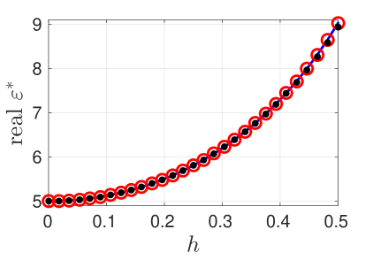
(a)

(b)

Figure 3: Dependence of the real (a) and imaginary (b) parts of the complex effective dielectric constant $\varepsilon^{\ast}$ of a square array of tubes on the parameter $\displaystyle h=a/\ell$. The solid blue line corresponds to exact numerical evaluation, red circles show result of formulas (14)–(15), and black dots represent Maxwell’s approximation (12) for $\varepsilon_{in}=2-4i$, $\varepsilon_{tu}=80-2i$, $\varepsilon_{ex}=5-4i$, and $\nu=0.9$.

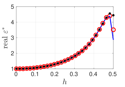
(a)

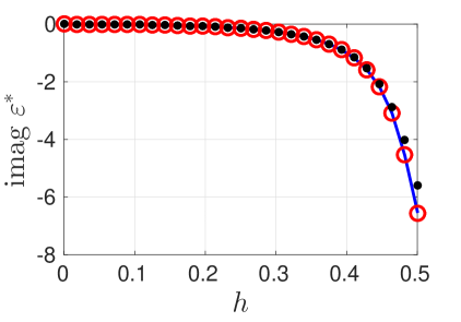
(b)

Figure 4: Dependence of the real (a) and imaginary (b) parts of the complex effective dielectric constant $\varepsilon^{\ast}$ of a hexagonal array of tubes on the parameter $\displaystyle h=a/\ell$. The solid blue line corresponds to exact numerical evaluation, red circles show result of formulas (14),(17), and black dots represent Maxwell’s approximation (12) for $\varepsilon_{in}=2-4i$, $\varepsilon_{tu}=8-40i$, $\varepsilon_{ex}=1$, and $\nu=0.9$.

Figures 3-4 show dependence of the real and imaginary parts of the complex effective dielectric constant $\varepsilon^{\ast}$ of a square and hexagonal arrays of tubes on the parameter $\displaystyle h=a/\ell$. Formula (14) gives an excellent agreement between numerical evaluation of $\varepsilon^{\ast}$ using solution of (29) and the expansions (15),(17) for chosen material parameters. In the case of square lattice estimate (37) gives $\|\mathcal{G}(0.5)\|_{\infty}\leqslant 1.4644$ while in fact $\|\mathcal{G}(0,5)\|_{\infty}\approx 0.88035$. For the hexagonal lattice estimation through (37) yields $\|\mathcal{G}(0.5)\|_{\infty}\leqslant 6.6122$ while direct evaluation results in $\|\mathcal{G}(0.5)\|_{\infty}\approx 1.1632$. Maxwell’s formula (12) gives a good approximation as long as the norm of the operator $\mathcal{G}(h)$ is significantly less than unity.

References

• [1] B. Y. Balagurov and V. A. Kashin, The conductivity of a 2d system with a doubly periodic arrangement of circular inclusions., Technical Physics, 46 (2001), pp. 101–106.
• [2] D. J. Bergman, Dielectric constant of a composite material – problem in classical physics, Physics Reports, 43 (1978), pp. 378–407.
• [3]  , Exactly solvable microscopic geometries and rigorous bounds for the complex dielectric-constant of a 2-component composite-material, Physical Review Letters, 44 (1980), pp. 1285–1287.
• [4]  , Bounds for the complex dielectric-constant of a 2-component composite-material, Physical Review B, 23 (1981), pp. 3058–3065.
• [5]  , Rigorous bounds for the complex dielectric constant of a two-component composite, Annals of Physics, 138 (1982), pp. 78–114.
• [6] P. Bisegna and F. Caselli, A simple formula for the effective complex conductivity of periodic fibrous composites with interfacial impedance and applications to biological tissues, Journal of Physics D: Applied Physics, (2008), p. 115506.
• [7] E. T. Copson, An Introduction to the Theory of Functions of a Complex Variable, Oxford University Press, 1948.
• [8] F. J. García-Vidal, J. M. Pitarke, and J. B. Pendry, Effective medium theory of the optical properties of aligned carbon nanotubes, Physical Review Letters, 78 (1997), pp. 4289–4292.
• [9] Yu. A. Godin, The effective conductivity of a periodic lattice of circular inclusions, Journal of Mathematical Physics, 53 (2012), p. 063703.
• [10]  , Effective complex permittivity tensor of a periodic array of cylinders, Journal of Mathematical Physics, 54 (2013), p. 053505.
• [11] K. Golden and G. Papanicolaou, Bounds for effective parameters of heterogeneous media by analytic continuation, Communications in Mathematical Physics, 90 (1983), pp. 473–491.
• [12]  , Bounds for effective parameters of multicomponent media by analytic continuation, Journal of Statistical Physics, 40 (1985), pp. 655–667.
• [13] E. I. Grigolyuk and L. A. Filshtinsky, Perforated plates and shells, Nauka, Moscow, 1970. (in Russian).
• [14] M. D. Guild, V. M. Garcia-Chocano, W. Kan, and J. Sánchez-Dehesa, Enhanced inertia from lossy effective fluids using multi-scale sonic crystals, AIP ADVANCES, 4 (2014), p. 124302.
• [15] H. Hancock, Lectures on the theory of elliptic functions, Dover, New York, 1958.
• [16] M. Maldovan, M. R. Bockstaller, E. L. Thomas, and W. C. Carter, Validation of the effective-medium approximation for the dielectric permittivity of oriented nanoparticle-filled materials: effective permittivity for dielectric nanoparticles in multilayer photonic composites, Applied Physics B, 76 (2003), pp. 877–884.
• [17] J. C. Maxwell, A Treatise on Electricity and Magnetism, Clarendon Press, Oxford, 1873.
• [18] R. C. McPhedran, Transport properties of cylinder pairs and of the square array of cylinders., Proceedings of the Royal Society of London A: Mathematical and Physical Sciences, 408 (1986), pp. 31–43.
• [19] G. W. Milton, Bounds on the complex dielectric constant of a composite material, Applied Physics Letters, 37 (1980), pp. 300–302.
• [20]  , Bounds on the complex permittivity of a two-component composite material, Journal of Applied Physics, 52 (1981), pp. 5286–5293.
• [21]  , Bounds on the transport and optical properties of a two-component composite material, Journal of Applied Physics, 52 (1981), pp. 5294–5304.
• [22] V. V. Mityushev, Transport properties of double-periodic arrays of circular cylinders., Zeitschrift für Angewandte Mathematik und Mechanik, 77 (1997), pp. 115–120.
• [23] N. A Nicorovici, R. C McPhedran, and G. W Milton, Transport properties of a three-phase composite material: the square array of coated cylinders, Proceedings of the Royal Society of London A: Mathematical and Physical Sciences, 442 (1993), pp. 599–620.
• [24] W. T. Perrins, D. R. McKenzie, and R. C. McPhedran, Transport properties of regular arrays of cylinders., Proceedings of the Royal Society of London A: Mathematical and Physical Sciences, 369 (1979), pp. 207–225.
• [25] Lord Rayleigh, On the influence of obstacles arranged in rectangular order upon the properties of a medium., Philosophical Magazine, 34 (1892), pp. 481–502.
• [26] E. Reyes, A. A. Krokhin, and J. Roberts, Effective dielectric constants of photonic crystal of aligned anisotropic cylinders and the optical response of a periodic array of carbon nanotubes, Physical Review B, 72 (2005), p. 155118.
• [27] N. Rylko, Transport properties of the rectangular array of highly conducting cylinders, Journal of Engineering Mathematics, 38 (2000), pp. 1–12.
• [28] V. V. Zalipaev, A. B. Movchan, C. G. Poulton, and R. C. McPhedran, Elastic waves and homogenization in oblique periodic structures, Proceedings of the Royal Society A: Mathematical, Physical and Engineering Sciences, 458 (2002), pp. 1887–1912.