meth \bibliographystylemethnaturemag-swj
Flows of X-ray gas reveal the disruption of a star by a massive black hole
Abstract
Tidal forces close to massive black holes can violently disrupt stars that make a close approach. These extreme events are discovered via bright X-ray[1, 2, 3, 4] and optical/UV[5, 6] flares in galactic centers. Prior studies based on modeling decaying flux trends have been able to estimate broad properties, such as the mass accretion rate[6, 7]. Here we report the detection of flows of highly ionized X-ray gas in high-resolution X-ray spectra of a nearby tidal disruption event. Variability within the absorption-dominated spectra indicates that the gas is relatively close to the black hole. Narrow line widths indicate that the gas does not stretch over a large range of radii, giving a low volume filling factor. Modest outflow speeds of are observed, significantly below the escape speed from the radius set by variability. The gas flow is consistent with a rotating wind from the inner, super-Eddington region of a nascent accretion disk, or with a filament of disrupted stellar gas near to the apocenter of an elliptical orbit. Flows of this sort are predicted by fundamental analytical theory[8] and more recent numerical simulations[9, 10, 11, 12, 7, 13, 14].
Department of Astronomy, The University of Michigan, 1085 South University Avenue, Ann Arbor, Michigan, 48103, USA.
SRON Netherlands Institute for Space Research, Sorbonnelaan 2, 3584 CA Utrecht, The Netherlands.
Department of Physics and Astronomy, Universiteit Utrecht, PO BOX 80000, 3508 TA Utrecht, The Netherlands.
Leiden Observatory, Leiden University, PO BOX 9513, 2300 RA Leiden, The Netherlands.
Department of Astronomy, The University of Maryland, College Park, Maryland, 20742, USA.
Department of Physics, University of Warwick, Coventry, CV4 7AL, UK.
Joint Space-Science Institute, University of Maryland, College Park, MD, 02742, USA.
Astrophysics Science Division, NASA Goddard Space Flight Center, MC 661, Greenbelt, Maryland, 20771, USA.
Smithsonian Astrophysical Observatory, 60 Garden Street, Cambridge, Massachusetts, 02138, USA.
The Institute for Theory and Computation, Harvard-Smithsonian Center for Astrophysics, 60 Garden Street, Cambridge, Massachusetts, 02138, USA.
Department of Physics and Astronomy, University of Alabama, BOX 870324, Tuscaloosa, Alabama, 35487, USA.
Department of Physics and Astronomy, Wheaton College, Norton, Massachusetts, 02766, USA.
Department of Physics and Astronomy, University of Leicester, University Road, Leicester, LE1 7RH, UK.
Columbia Astrophysics Laboratory and Department of Astronomy, Columbia University, 550 West 120th Street, New York, New York, 10027, USA.
Department of Astronomy and Astrophysics, University of California, Santa Cruz, California, 95064, USA.
ASASSN-14li was discovered in images obtained on November 22, 2014 (MJD 56983), at a visual magnitude of V=16.5[15] by the All-Sky Automated Survey for Supernovae (ASAS-SN). Follow-up observations found the transient source to coincide with the center of the galaxy PGC 043234 (originally Zw VIII 211), to within 0.04 arc seconds[15]. This galaxy lies at a red-shift of , or a luminosity distance of 90.3 Mpc (for , , ), making ASASSN-14li the closest disruption event discovered in over 10 years. The discovery magnitudes indicated a substantial flux increase over prior, archival optical images of this galaxy. Follow-up observations with the Swift X-ray Telescope[16, 17] (XRT) established a new X-ray source at this location[15].
Archival X-ray studies rule out the possibility that PGC 043234 harbours a standard active galactic nucleus that could produce bright flaring. PGC 043234 is not detected in the ROSAT All-Sky Survey[18]. Utilizing the online interface to the data, the background count rate for sources detected in the vicinity is . With standard assumptions (see Methods), this rate corresponds to a luminosity of , which is orders of magnitude below a standard active nucleus.
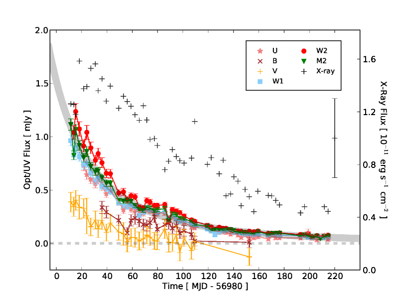
Theory predicts that early tidal disruption event (TDE) evolution should be dominated by a bright, super-Eddington accretion phase, and be followed by a charactecteristic decline as disrupted material interacts and accretes[8, 19]. Detections of winds integral to super-Eddington accretion have not been reported previously, but flux decay trends in the UV (where disk emission from active nuclei typically peaks) are now a standard signature of TDEs in the literature[5, 6]. Figure 1 shows the flux decay of ASASSN-14li, as observed by Swift. A fit to the UVM2 data assuming an index of gives a disruption date of (MJD). The V-band light is consistent with a shallower decay; this can indicate direct thermal emission from the disk, or reprocessed emission[11, 7] (see Methods).
We triggered approved XMM-Newton programs to study ASASSN-14li soon after its discovery. Although XMM-Newton carries several instruments, the spectra from the two RGS units are the focus of this analysis. We were also granted a Director’s Discretionary Time observation with Chandra, using its Low Energy Transmission Grating spectrometer (LETG), paired with its High Resolution Camera for spectroscopy (HRC-S).
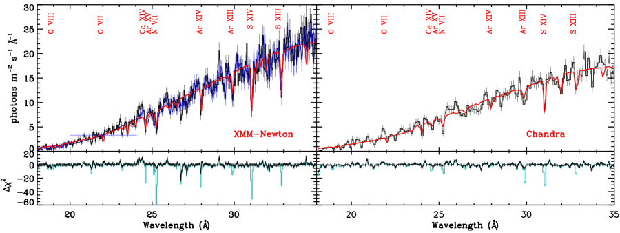
The 18–35Å X-ray spectra of ASASSN-14li are clearly thermal in origin, so we modeled the continuum with a single blackbody, modified by interstellar absorption in PGC 043234 and the Milky Way, and absorption from blue-shifted, ionized gas local to the TDE. The self-consisent photoionization code “pion”[20] was used to model the complex absorption spectra (see Table 1, and Methods).
Assuming that the highest bolometric luminosity derived in fits to the high-resolution spectra () corresponds to the Eddington limit, a black hole mass of is inferred. The blackbody emission measured in fits to the time-averaged XMM-Newton spectrum gives an emitting area of ; implying for a spherical geometry. This is consistent with the innermost stable circular orbit (ISCO) around an black hole. Modeling of the Swift light curves (see Figure 1) using a self-consistent treatment of direct and reprocessed light from an elliptical accretion disk[7] gives a mass in the range of (please see the Methods). In concert, the thermal spectrum, implied radii, and the run of emission from X-rays to optical bands unambiguously signal the presence of an accretion disk in ASASSN-14li.
Figure 2 shows the best-fit model for the spectra obtained in the long stare with the XMM-Newton/RGS (see Table 1, and Methods). An F-test finds that photoionized X-ray absorption is required in fits to these spectra at more than the 27 level of confidence, relative to a spectral model with no such absorption. The model captures the majority of the strong absorption lines, giving for 563 degrees of freedom (see Table 1). The strongest lines in the spectrum coincide with ionized charge states of N, O, S, Ar, and Ca. Only solar abundances are required to describe the spectra. The Chandra spectrum independently confirms these results in broad terms, and requires absorption at more than the 6 level of confidence.
A hard lower limit on the radius of the absorbing gas is set by the the blackbody continuum. The best radius estimate likely comes from variability time scales within the XMM-Newton long stare. Analysis of specific time segments within the long stare, as well as flux-selected segments, reveals that the absorption varies (see Table 1, and Methods). This sets a relevant limit of , or . While the column density and ionization do not vary significantly, the blue-shift of the gas does. During the initial third of the observation, the blue-shift is larger, , but falls to in the final two-thirds. Shorter monitoring observations with XMM-Newton reveal evolution of the absorbing gas, including changes in ionization and column density, before and after the long stare (see Table 1, and Methods).
Fundamental theoretical treatments of TDEs predict an initial near-Eddington or super-Eddington phase[8]; this is confirmed in more recent theoretical studies[21, 9, 12]. The high-resolution X-ray spectra were obtained within the predicted time frame for super-Eddington accretion, for our estimates of the black hole mass[22]. Although the ionization parameter of the observed gas is high, the ionizing photon distribution peaks at a low energy, and the wind could be driven by radiation force. Such flows are naturally clumpy, and may be similar to the photospheres of novae[23]. Given the strong evidence of an accretion disk in our observations of ASASSN-14li, the X-ray outflow is best associated with a wind from the inner regions of a nascent, super-Eddington accretion disk. The local escape speed at an absorption radius of (appropriate for ) exceeds the observed outflow line-of-signt speed of the gas, but Keplerian rotation is not encoded in absorption, and projection effects are also important. The small width of the absorption lines relative to the escape velocity may also indicate a low filling factor, consistent with a clumpy outflow or shell.
The existing observations show a general trend toward higher outflow speeds with time. Corresponding changes in ionization and column density are more modest, and not clearly linked to outflow speed[24]. However, some recent work has predicted higher outflow speeds in an initial super-Eddington disk regime, and lower outflow speeds in a subsequent thin disk regime[9, 12]. An observation in an earlier, more highly super-Eddington phase might have observed broader lines and higher outflow speeds; future observations of new TDEs can test this.
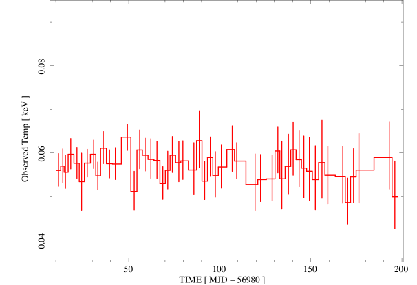
Figure 3 shows the time evolution of the blackbody temperature measured in Swift/XRT monitoring observations. The temperature is remarkably constant, especially in contrast to the optical/UV decline shown in Figure 1. Observations of steady blackbody temperatures despite decaying multi-wavelength light curves in some TDEs[6, 25] has recently been explained through winds[14]. Evidence of winds in our data supports this picture.
The low gas velocities may also be consistent with disrupted stellar gas on an elliptical orbit in a nascent disk, near apocenter. This picture naturally gives a low filling factor, resulting in a small total mass in absorbing gas (see Methods). Recent numerical simulations predict that a fraction of the disrupted material in a TDE will circularize slowly[13], and that flows will be filamentary[26], while stellar gas that is more tightly bound can form an inner, Eddington-limited or super-Eddington disk more quickly.
The highly ionized, blue-shifted gas discovered in our high-resolution X-ray spectra of ASASSN-14li confirms both fundamental and very recent theoretical predictions for the structure and evolution of tidal disruption events. The field can now proceed to pair high-resolution X-ray spectroscopy with an ever-increasing number of TDE detections to test models of accretion disk formation and evolution, and to explore strong-field gravitation around massive black holes[27].
References
- [1] Bade, N., Komossa, S. & Dahlem, M. Detection of an extremely soft X-ray outburst in the HII-like nucleus of NGC 5905. Astron. Astrophys. 309, L35–L38 (1996).
- [2] Komossa, S. & Greiner, J. Discovery of a giant and luminous X-ray outburst from the optically inactive galaxy pair RX J1242.6-1119. Astron. Astrophys. 349, L45–L48 (1999).
- [3] Esquej, P. et al. Candidate tidal disruption events from the XMM-Newton slew survey. Astron. Astrophys. 462, L49–L52 (2007).
- [4] Cappelluti, N. et al. A candidate tidal disruption event in the Galaxy cluster Abell 3571. Astron. Astrophys. 495, L9–L12 (2009).
- [5] Gezari, S. et al. UV/Optical Detections of Candidate Tidal Disruption Events by GALEX and CFHTLS. Astrophys. J. 676, 944–969 (2008).
- [6] Gezari, S. et al. An ultraviolet-optical flare from the tidal disruption of a helium-rich stellar core. Nature 485, 217–220 (2012).
- [7] Guillochon, J., Manukian, H. & Ramirez-Ruiz, E. PS1-10jh: The Disruption of a Main-sequence Star of Near-solar Composition. Astrophys. J. 783, 23 (2014).
- [8] Rees, M. J. Tidal disruption of stars by black holes of 10 to the 6th-10 to the 8th solar masses in nearby galaxies. Nature 333, 523–528 (1988).
- [9] Strubbe, L. E. & Quataert, E. Optical flares from the tidal disruption of stars by massive black holes. Mon. Not. R. Astron. Soc. 400, 2070–2084 (2009).
- [10] Lodato, G., King, A. R. & Pringle, J. E. Stellar disruption by a supermassive black hole: is the light curve really proportional to t-5/3? Mon. Not. R. Astron. Soc. 392, 332–340 (2009).
- [11] Lodato, G. & Rossi, E. M. Multiband light curves of tidal disruption events. Mon. Not. R. Astron. Soc. 410, 359–367 (2011).
- [12] Strubbe, L. E. & Quataert, E. Spectroscopic signatures of the tidal disruption of stars by massive black holes. Mon. Not. R. Astron. Soc. 415, 168–180 (2011).
- [13] Shiokawa, H., Krolik, J. H., Cheng, R. M., Piran, T. & Noble, S. C. General Relativistic Hydrodynamic Simulation of Accretion Flow from a Stellar Tidal Disruption. arxiv:1501.04365 (2015).
- [14] Miller, M. C. Disk Winds as an Explanation for Slowly Evolving Temperatures in Tidal Disruption Events. arxiv:1502.03284 (2015).
- [15] Jose, J. et al. ASAS-SN Discovery of an Unusual Nuclear Transient in PGC 043234. The Astronomer’s Telegram 6777, 1 (2014).
- [16] Gehrels, N. et al. The Swift Gamma-Ray Burst Mission. Astrophys. J. 611, 1005–1020 (2004).
- [17] Burrows, D. N. et al. The Swift X-Ray Telescope. Space Science Reviews 120, 165–195 (2005).
- [18] Voges, W. et al. The ROSAT all-sky survey bright source catalogue. Astron. Astrophys. 349, 389–405 (1999).
- [19] Phinney, E. S. Manifestations of a Massive Black Hole in the Galactic Center. In Morris, M. (ed.) The Center of the Galaxy, vol. 136 of IAU Symposium, 543 (1989).
- [20] Kaastra, J. S., Mewe, R. & Nieuwenhuijzen, H. SPEX: a new code for spectral analysis of X and UV spectra. In Yamashita, K. & Watanabe, T. (eds.) UV and X-ray Spectroscopy of Astrophysical and Laboratory Plasmas, 411–414 (1996).
- [21] Loeb, A. & Ulmer, A. Optical Appearance of the Debris of a Star Disrupted by a Massive Black Hole. Astrophys. J. 489, 573–578 (1997).
- [22] Piran, T., Svirski, G., Krolik, J., Cheng, R. M. & Shiokawa, H. Disk Formation Versus Disk Accretion - What Powers Tidal Disruption Events? Astrophys. J. 806, 164 (2015).
- [23] Shaviv, N. J. The theory of steady-state super-Eddington winds and its application to novae. Mon. Not. R. Astron. Soc. 326, 126–146 (2001).
- [24] Ramírez, J. M. Kinematics from spectral lines for AGN outflows based on time-independent radiation-driven wind theory. Rev. Mexicana Astron. Astrofis. 47, 385–399 (2011).
- [25] Holoien, T. W.-S. et al. ASASSN-14ae: a tidal disruption event at 200 Mpc. Mon. Not. R. Astron. Soc. 445, 3263–3277 (2014).
- [26] Guillochon, J. & Ramirez-Ruiz, E. A Dark Year for Tidal Disruption Events. arxiv:1501.05306 (2015).
- [27] Stone, N. & Loeb, A. Observing Lense-Thirring Precession in Tidal Disruption Flares. Physical Review Letters 108, 061302 (2012).
- [28] Kaastra, J. S., Mewe, R. & Raassen, T. New Results on X-ray Models and Atomic Data. Highlights of Astronomy 13, 648 (2005).
We thank Chandra Director Belinda Wilkes and the Chandra team for accepting our request for Director’s Discretionary Time, XMM-Newton Director Norbert Schartel and the XMM-Newton team for executing our approved target-of-opportunity program, and Swift Director Neil Gehrels and the Swift team for monitoring this important source. J.M.M. is supported by NASA funding, through Chandra and XMM-Newton guest observer programs. SRON is supported by NWO, the Netherlands Organization for Scientific Research. JJD was supported by NASA Contract NAS8-03060 to the Chandra X-ray Center. W.P.M. is grateful for support by the University of Alabama Research Stimulation Program.
J.M.M. led the Chandra and XMM-Newton data reduction and analysis, with contributions from J.S.K., J.J.D., and J.P. M.R. led the Swift data reduction and analysis, with help from B.C., S.G, and R.M. M.C.M., E.R.-R., and J.G. provided theoretical insights. G.B., K.G., J.I., A.L., D.M., W.P.M., P.O., D.P., F.P., T.S., and N.T. contributed to the discussion and interpretation.
The authors declare that they have no competing financial interests.
Correspondence and requests for materials should be addressed to J.M.M. (jonmm@umich.edu).
| Mission | XMM-Newton | XMM-Newton | XMM-Newton | XMM-Newton | Chandra | XMM-Newton |
|---|---|---|---|---|---|---|
| ObsId | 0694651201 | 0722480201 | 0722480201 | 0722480201 | 17566, 17567 | 0694651401 |
| comment | monitoring | long stare | stare (low) | stare (high) | – | monitoring |
| Start (MJD) | 56997.98 | 56999.54 | 56999.94 | 57000.0 | 56999.97, 57002.98 | 57023.52 |
| Duration (ks) | 22 | 94 | 36 | 58 | 35, 45 | 23.6 |
| () | ||||||
| () | ||||||
| () | ||||||
| () | ||||||
| 2.6* | 2.6* | 2.6* | 2.6* | 2.6* | ||
| 1.4* | 1.4* | 1.4* | 1.4* | 1.4* | ||
| log() (erg cm s-1) | ||||||
| (km ) | ||||||
| (km ) | ||||||
| kT (eV) | ||||||
| Norm () | ||||||
| 704.8/567 | 870.5/563 | 687.8/564 | 726.8/565 | 266.5/178 | 626.5/566 |
Methods
Estimates of prior black hole luminosity
Utilizing the ROSAT All-Sky Survey\citemethVoges99, the region
around the host galaxy, PGC 043234, was searched for
point sources. No sources were found. Points in the vicinity of the
host galaxy were examined to derive a background count rate of 0.002
counts . Assuming the Milky Way column density along
this line of sight, and taking a typical Seyfert X-ray spectral index
of , this count rate translates into . This limit is orders of magnitude
below a Seyfert or quasar luminosity.
Optical/UV monitoring observations and data reduction
Swift\citemethGehrels04 monitors transient and variable sources via co-aligned X-ray (XRT: 0.3 - 10 keV) and UV-Optical (UVOT: 170-650 nm) telescopes. High-cadence monitoring of ASASSN-14li with UVOT has continued in six bands: V, B, U, UVW1, UVM2, and UVW2 ().
All observations were processed using the latest HEASOFT suite and calibrations. Individual optical/UV exposures were astrometrically corrected and sub-exposures in each filter were summed. Source fluxes were then extracted from an aperture of 3′′radius, and background fluxes were extracted from a source-free region to the east of ASASSN-14li due to the presence of a (blue) star lying 10 arc seconds to the South, using uvotmaghist.
To estimate the host contamination, we have measured the host flux in 3′′aperture (matched to the aperture used for the UVOT photometry) in pre-outburst Sloan Digital Sky Survey (SDSS; \citemethaaa14), 2 Micron All-Sky Survey (2MASS; \citemethscs06), and GALEX \citemethmfs05 images. Extra caution was used to deblend the GALEX data, where large PSF resulted in contamination from the star ′′to the South. We estimated the uncertainty in each host flux by varying the inclusion aperture from 2′′to 4′′.
We then fit the host photometry to synthetic galaxy templates using the Fitting and Assessment of Synthetic Templates (FAST; \citemethkvl09) code. We employed stellar templates from the \citemethbc03 catalog, and allowed the star formation history, extinction law, and initial mass function to vary over the full range of parameters allowed by the software. All best fit models had stellar masses , low ongoing star formation rates (SFR yr-1), and modest line-of-sight extinction ( mag).
We took the resulting galaxy template spectra and integrated these over each UVOT filter bandpass to estimate the host count rate. For the uncertainty in this value, we adopt either the root-mean-square spread of the resulting galaxy template models, or 10% of the inferred count rate, whichever value was larger. We then subtracted these values from our measured (coincidence-loss corrected) photometry of the host plus transient, to isolate the component due to TDE. For reference, our inferred count rates for each UVOT filter are: s-1, s-1, s-1, s-1, s-1, and s-1.
Figure 1 shows the host-subtracted optical and UV light curves ASASSN-14li.
Fits to the UVOT/UVM2 light curve
The UVM2 filter provides the most robust trace of the mass accretion rate in a TDE like ASASSN-14li; it has negligible transmission at optical wavelengths\citemethPoole08,Breeveld11. Fits to the UVM2 light curve with a power-law of the form with a fixed index of imply a disruption date of (MJD). This model achieves a fair characterization of the data; high fluxes between days 80-100 (in the units of Figure 1) result in a poor statistical fit (, where degrees of freedom). If the light curve is fit with a variable index, a value of is measured (90% confidence). This model achieves an improved fit (, for degrees of freedom), but it does not tightly constrain the disruption date, placing in the MJD 56855–56920 range. That disruption window is adjacent to an interval wherein the ASAS-SN monitoring did not detect the source[15], making it less plausible than the fit with .
The optical bands appear to have a shallower decay curve than the UV
bands. Recent theory\citemethLodato11 predicts that optical light
produced via thermal disk emission should show a decay consistent with
; this might also be due to
reprocessing\citemethGuillochon:2014a. The V-band data are
consistent with this prediction, though the data are of modest quality
and a broad range of decays are permitted.
X-ray monitoring observations and data reduction
The Swift/XRT\citemethBurrows05 is a charge-coupled device (CCD). In such cameras, photon pile-up occurs when two or more photons land within a single detection box during a single frame time. This causes flux distortions and spectral distortions to bright sources. Such distortions are effectively avoided by extracting events from an annular region, rather than from a circle at the center of the telescope PSF. We therefore extracted source spectra from annuli with an inner radius of 12 arc seconds (5 pixels), and an outer radius of 50 arc seconds. Background flux was measured in annular region extending from 140 – 210 arc seconds.
Standard redistribution matrices were used; an ancillary response file was created with the xrtmkarf tool utilizing a vignetting corrected exposure map. The source spectra were rebinned to have 20 counts per bin with grppha. In all spectral fits, we adopted a lower spectral bound of 0.3 keV (36 ). The upper bound on spectral fits varied depending on the boundary of the last bin with at least 20 counts; this was generally around 1 keV (12 ).
The XRT spectra were fit with a model consisting of absorption in the Milky Way of a blackbody emitted at the redshift of the TDE, i.e., pha(zashift(bbodyrad)), where and . The evolution of the best-fit temperature of this blackbody component is displayed in Figure 3.
The blackbody temperature values measured from the
Swift/XRT are slightly higher (kT 7–10 eV) than those
measured with XMM-Newton and Chandra. If an outflow
component with fiducial parameters is included in the spectral model
anyway, the XRT temperatures are then in complete agreement with those
measured using XMM-Newton and Chandra.
Estimates of the black hole mass
Luminosity values inferred for the band over which the high-resolution spectra are actually fit, and a broader band are listed in Table 1. Taking the broader values as a proxy for a true bolometric fit, the highest implied soft X-ray luminosity is measured in the last XMM-Newton monitoring observation, giving . The Eddington luminosity for standard hydrogen-rich accretion is . This implies a black hole mass of .
Blackbody continua imply size scales, and - assuming that optically thick blackbody emission can only originate at radii larger than the innermost stable circular orbit (ISCO) - therefore masses. For a non-spinning Schwarzschild black hole, . The blackbody emission measured in fits to the time-averaged XMM-Newton “long stare” gives an emitting area of ; implying for a spherical geometry. The actual geometry may be more disk-like, but the inner flow may be a thick disk that is better represented by a spherical geometry. If the black hole powering ASASSN-14li is not spinning, this size implies a black hole mass of .
We also estimated the mass of the black hole at the heart of ASASSN-14li by fitting the host-subtracted light curves (see Figure 1) using the Monte Carlo software TDEFit \citemethGuillochon:2014a. This software assumes that emission is produced within an elliptical accretion disk where the mass accretion rate follows the fallback rate \citemethGuillochon:2013a onto the black hole with a viscous delay \citemethGuillochon:2015b. This emission is then partly reprocessed into the UV/optical by an optically thick layer \citemethLoeb:1997a. Super-Eddington accretion is treated by presuming a fitted fraction of the Eddington excess is converted into light that is reprocessed by the same optically thick layer. This excess can be produced either with an unbound wind \citemethStrubbe:2009a,Vinko:2015a, or with the energy deposited by shocks in the circularization process \citemethShiokawa:2015a,Piran:2015c.
The software performs a maximum-likelihood analysis to determine the
combinations of parameters that reproduce the observed light curves.
We utilize the ASASSN, UVOT, and XRT data in our light-curve fitting;
the most-likely models produce good fits to all bands simultaneously.
Within the context of this TDE model, a black hole mass of
0.4–1.2 (1) is dervived.
Spectroscopic observations, data reduction, and analysis
Table 1 lists the observation identification number (ObsId), start time, and duration of all of the XMM-Newton and Chandra observations considered in our work.
The XMM-Newton data were reduced using the standard Science Analysis System (SAS version 13.5.0) tools and the latest calibration files. The “rgsproc” routine was used to generate spectral files from the source, background spectral files, and instrument response files. The spectra from the RGS-1 and RGS-2 units were fit jointly. Prior to fitting models, all XMM-Newton spectra were binned by a factor of five for clarity and sensitivity.
The Chandra data were reduced using the standard Chandra Interactive Analysis of Observations (CIAO version 4.7) suite, and the latest associated calibration files. Instrument response files were constructed using the “fullgarf” and “mkgrmf” routines. The first-order spectra from each observation were combined using the tool “add_grating_orders”, and spectra from each observation were then added using “add_grating_spectra”.
The spectra were analyzed using the “SPEX” suite version 2.06[20]. The fitting procedure minimized a statistic. The spectra are most sensitive in the 18–35 Å band, and all fits were restricted to this range. Within SPEX, absorption from the interstellar medium in the Milky Way was modeled using the model “hot”; a separate “hot” component was included to allow for ISM absorption within PGC 043234 at its known red-shift (using the “reds” component in SPEX). The photoionized outflow was modeled using the “pion” component within the SPEX suite.
Pion[20] includes numerous lines from intermediate charge states that are lacking in similar astrophysics packages. The fits explored in this analysis varied the gas column density (), the gas ionization parameter (, where , and is luminosity, is the hydrogen number density, and is the distance between the ionizing source and absorbing gas), the rms velocity of the gas (), and the bulk shift of the gas relative to the source, in the source frame ().
Spectra from segments within the “long stare” made with XMM-Newton were made by using the SAS tool “tabgtigen” to create “good time interval” files to isolate periods within the light curves of the RGS data.
The Chandra/LETG spectra were dispersed onto the HRC, which has a relatively high instrumental background. Fitting the spectra only in the 18–35Å band served to limit the contributions of background. Nevertheless, the Chandra spectra are less sensitive than the best XMM-Newton spectra of ASASSN-14li (see Figure 2). Prior to fitting, spectra from the two exposures were added and then binned by a factor of three.
Figure 2 includes plots of the goodness-of-fit statistic as a function of wavelength, before and after including pion to model the ionized absortpion. There is weak evidence of emission lines in the spectra, perhaps with a P-Cygni profile (see below). The best-fit models for the high-resolution spectra predict one absorption line at 34.5Å (H-like C VI) that is not observed; small variations to abundances could resolve this disparity.
Blue-shifts as small as are measured in the XMM-Newton/RGS using the pion model. According to the XMM-Newton User’s Handbook, available through the mission website, the absolute accuracy of the first-order wavelength scale is 6 mÅ. At 18 Å, this corresponds to a velocity of ; at 35 Å, this corresponds to a velocity of . The model predicts numerous lines across the 18–35 Å band that are clearly detected; especially with this leverage, the small shifts we have measured with XMM-Newton are robust. In particular, the difference in blue-shift between the low and high flux phases of the long stare, versus , is greater than absolute calibration uncertainties. Differences observed in the outflow velocities between XMM-Newton observations are as large, or larger, and also robust.
The lower sensitivity of the Chandra spectra is evident in the relatively poor constraints achieved on the column density of the ionized X-ray outflow (see Table 1). Similarly, the relatively high outflow velocity measured in the Chandra spectra, should be viewed with a degree of caution. The outflow velocity changes from to just , for instance, when the binning factor is increased from three to five. We have found no reports in the literature of a systematic wavelength offset between contemporaneous high-resolution spectra obtained with XMM-Newton and Chandra.
The small number of high-resolution spectra complicates efforts to
discern trends. The velocity width of the absorbing gas is fairly
constant over time, but there is a general trend toward higher
blue-shifts. There is no clear trend in column density or ionization
parameter with time.
Diffuse gas mass, outflow rates, and filling factors
There is no a priori constraint on the density of the absorbing gas. Taking the maximum radius implied by variability within XMM-Newton long stare, , and manipulating the ionization parameter equation (, where is the luminosity, is the number density, and is the absorbing radius), we can derive an estimate of the density: . Even assuming a uniformly-filled sphere out to a radius of , a total mass of is implied, or approximately .
The true gas mass within is likely to be orders of magnitude lower, owing to clumping and a very low volume filling factor. Using the measured value of and assuming , gives a value of . The filling factor can be estimated via . The total mass enclosed out to a distance is then reduced accordingly, down to , assuming a uniform density within . This is a small value, plausible either for a clumpy wind or gas within a filament executing an elliptical orbit.
Formally, the mass outflow rate in ASASSN-14li can be adapted from the case where the density is known, and written as:
,
where is the mean atomic weight ( is
typical), is the mass of the proton, is the covering
factor (), is the ionizing luminosity,
is the outflow velocity, is the line-of-sight global
filling factor, and is the ionization parameter. Using the
values obtained in fits to the XMM-Newton long stare (see Table
1), for instance, . Taking the value of derived
above, an outflow rate of results. The kinetic power in the
outflow is given by ; using the same
values assumed to estimate the mass outflow rate, .
Emission from the diffuse outflow
We synthesized a plausible wind emission spectrum by coupling the pion and “hyd” models within SPEX. They hyd code enables spectra to be constructed based on the output of hydrodynamical simulations. As inputs, it requires the electron temperature and ion concentrations for a gas; these were taken from our fits with pion. We included the resulting emission component in experimental fits to the XMM-Newton long stare. The best-fit model gives an emission measure of , a red-shift (relative to the host) of , and an ionization parameter of log.
Via an F-test, the emission component is only required at the level; however, it has some compelling properties. Combined with the blue-shifted absorption spectrum, the red-shifted emission gives P-Cygni profiles. For the gas density of derived previously, the emission measure gives a radius of , comparable to the size scale inferred from absorption variability.
The strongest lines predicted by the emission model include He-like O
VII, and H-like charge states of C, N, and O. This model does not
account for other emission line-like features in the spectra, which
are more likely to be artifacts from spectral binning, or calibration
or modeling errors. Emission features in the O K-edge region may be
real, but caution is warranted. Other features are more easily
discounted as they differ between the RGS-1 and RGS-2 spectra.
Code Availability
All of the data reduction and spectroscopic fitting routines and packages used in this work are publicly available.
The light curve modeling package, TDEFit \citemethGuillochon:2014a, is proprietary at this time owing to ongoing code development; a public release is planned within the coming year.
meth