Coupling regularization and adaptive $hp$-BEM for the solution of a delamination problem

Abstract

In this paper, we couple regularization techniques with the adaptive $hp$-version of the boundary element method ($hp$-BEM) for the efficient numerical solution of linear elastic problems with nonmonotone contact boundary conditions. As a model example we treat the delamination of composite structures with a contaminated interface layer. This problem has a weak formulation in terms of a nonsmooth variational inequality. The resulting hemivariational inequality (HVI) is first regularized and then, discretized by an adaptive $hp$-BEM. We give conditions for the uniqueness of the solution and provide an a-priori error estimate. Furthermore, we derive an a-posteriori error estimate for the nonsmooth variational problem based on a novel regularized mixed formulation, thus enabling $hp$-adaptivity. Various numerical experiments illustrate the behavior, strengths and weaknesses of the proposed high-order approximation scheme.

1 Introduction

The interest in robust and efficient numerical methods for the solution of nonsmooth problems in nonmonoton contact like adhesion and delamination problems increases constantly. The nonsmoothness comes from the nonsmooth data of the problems itself, in particular from nonmonotone multivalued physical laws involved in the boundary conditions that lead to nonsmooth functionals in the variational formulation. There are several approaches to treat this non-differentiability. We can first discretize by finite elements, and then solve the nonconvex optimization problems by novel nonsmooth optimization methods Noll_Ovcharova , or first regularize the nonsmooth functional, then discretize by finite element methods and finally use standard optimization solvers Ovcharova2012 . Since the interesting nonmonotone behavior takes place only in a boundary part of the involved linear elastic bodies, the domain hemivariational inequaliy can also be formulated as a boundary hemivariational inequality via the Poincaré-Steklov operator. Therefore, the boundary element methods (BEM) are the methods of choice for discretization. There are number of works exploiting the $h$- and the high-order $hp$-version of the BEM for monotone contact problems. Advanced $hp$-BEM discretizations, a-priori and a-posteriori error estimates for unilateral Signorini problems or contact problems with monotone friction are established in banz2013posteriori ; Banz2015 ; chernov2008hp ; MS-1 ; maischak2007adaptive ; stephan2009hp . However, successfully applied $hp$-BEM techniques for nonsmooth nonconvex variational inequalities are still missing. Pure $h$-BEM with lowest polynomial degree has been investigated for the first time by Nesemann and Stephan Nesemann for unilateral contact with adhesion. They study the existence and uniqueness, and introduce a residual error indicator.

In this paper, we extend the approximation scheme from Ovcharova2015 (dealing with the $h$ - version of the BEM) to the $hp$-version of the BEM for the regularized problem. More precisely, the nonsmooth variational inequality is first regularized and then discretized by $hp$-adaptive BEM. For the Galerkin solution of the regularized problem we provide an a-priori error estimate and derive a reliable a-posteriori error estimate based on a novel regularized mixed formulation and thus, enabling $hp$-adaptivity. All our theoretical results are illustrated with various numerical experiments for a contact problem with adhesion. We also provide conditions for the uniqueness of the solution that sharpen the results due to Nesemann .

Notation: We denote with $C_{i}$, $c_{i}$ and such alike generic constants, which can take different values at different positions. We use bold font to indicate vector-valued variables, e.g. $\mathbf{u}\in\mathbf{H}^{1}(\Omega):=[H^{1}(\Omega)]^{d}$. If there are too many indices, one of them is written as a superscript, e.g. $\mathbf{u}_{\varepsilon,hp}=\mathbf{u}^{\varepsilon}_{hp}$.

2 A nonmonotone boundary value problem from delamination

Let $\Omega\subset\mathbb{R}^{d}\,(d=2,3)$ be a bounded domain with Lipschitz boundary $\Gamma=\partial\Omega$. We assume that the boundary is decomposed into three disjoint open parts $\Gamma_{D},\Gamma_{N}$, and $\Gamma_{C}$ such that $\Gamma=\overline{\Gamma}_{D}\cup\overline{\Gamma}_{N}\cup\overline{\Gamma}_{C}$ and, moreover, the measures of $\Gamma_{C}$ and $\Gamma_{D}$ are positive. We fix an elastic body occupying $\overline{\Omega}$. The body is subject to volume force ${\mathbf{f}}\in[L^{2}(\Omega)]^{d}$ and $g\in H^{1/2}(\Gamma_{C})$, $g\geq 0$, is a gap function associating every point $x\in\Gamma_{C}$ with its distance to the rigid obstacle measured in the direction of the unit outer normal vector $\mathbf{n}(x)$. The body is fixed along $\Gamma_{D}$, surface tractions $\mathbf{t}\in[L^{2}(\Gamma_{N})]^{d}$ act on $\Gamma_{N}$, and on the part $\Gamma_{C}$ a nonmonotone, generally multivalued boundary condition holds.

Further, $\varepsilon(\mathbf{u})=\frac{1}{2}(\nabla{\mathbf{u}}+\nabla{\mathbf{u}}^{T})$ denotes the linearized strain tensor and $\sigma(\mathbf{u})=\mathcal{C}\,:\,\varepsilon(\mathbf{u})$ stands for the stress tensor, where $\mathcal{C}$ is the Hooke tensor, assumed to be uniformly positive definite with $L^{\infty}$ coefficients. The boundary stress vector can be decomposed further into the normal, respectively, the tangential stress:

$$\sigma_{n}=\sigma(\mathbf{u}){\mathbf{n}}\cdot{\mathbf{n}},\quad\sigma_{t}=\sigma(\mathbf{u}){\mathbf{n}}-\sigma_{n}{\mathbf{n}}.$$

By assuming that the structure is symmetric and the forces applied to the upper and lower part are the same, it suffices to consider only the upper half of the specimen represented by $\overline{\Omega}$, see Fig. 2 left for the 2D benchmark problem.

 

(a) Load-displacement curve for different contamination concentrations, see Gudladt

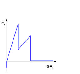
(b) A nonmonotone adhesion law

Figure 1: Nonmonotone adhesion law

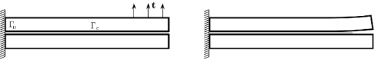
Figure 2: Reference configuration for the 2D benchmark under loading. Under applied traction force $\mathbf{t}$ the crack front propagates to the left

The delamination problem under consideration is the following: Find ${\mathbf{u}}\in\mathbf{H}^{1}(\Omega):=[H^{1}(\Omega)]^{d}$ such that

$$-\mbox{div}\;\sigma({\mathbf{u}}) ={\mathbf{f}} \mbox{in}\;\Omega$$ (1a)

$${\mathbf{u}} =0 \mbox{on}\;\Gamma_{D}$$ (1b)

$$\sigma({\mathbf{u}}){\mathbf{n}} ={\mathbf{t}} \mbox{on}\;\Gamma_{N}$$ (1c)

$$u_{n} \leq g \mbox{on}\;\Gamma_{C}$$ (1d)

$$\sigma_{t}({\mathbf{u}}) =0 \mbox{on}\;\Gamma_{C}$$ (1e)

$$-\sigma_{n}({\mathbf{u}}) \in\partial f(u_{n}) \mbox{on}\;\Gamma_{C}.$$ (1f)

The contact law (1f), written as a differential inclusion by means of the Clarke subdifferential $\partial f$ Clarke of a locally Lipschitz function $f$, describes the nonmonotone, multivalued behavior of the adhesive. More precisely, $\partial f$ is the physical law between the normal component $\sigma_{n}$ of the stress boundary vector and the normal component $u_{n}=\mathbf{u}\cdot\mathbf{n}$ of the displacement $\mathbf{u}$ on $\Gamma_{C}$. A typical zig-zagged nonmonotone adhesion law is shown in Figure 1(b).
To give a variational formulation of the above boundary value problem we define

$$\mathbf{H}^{1}_{D}(\Omega)=\left\{\mathbf{v}\in\mathbf{H}^{1}(\Omega)\,:\,\mathbf{v}|_{\Gamma_{D}}=0\right\},\quad\mathcal{K}=\{\mathbf{v}\in\mathbf{H}^{1}_{D}(\Omega)\,:\,v_{n}\leq g\text{ a.e.~{}on }\Gamma_{C}\}$$

and introduce the $\mathbf{H}^{1}_{D}(\Omega)$-coercive and continuous bilinear form of linear elasticity

$$a(\mathbf{u},\mathbf{v})=\int_{\Omega}\sigma(\mathbf{u}):\varepsilon(\mathbf{v})\,dx.$$

Multiplying the equilibrium equation (1a) by $\mathbf{v-u}$, integrating over $\Omega$ and applying the divergence theorem yields

$$\int_{\Omega}\sigma(\mathbf{u}):\varepsilon(\mathbf{v}-\mathbf{u})\,dx=\int_{\Omega}\mathbf{f}\cdot(\mathbf{v}-\mathbf{u})\,dx+\int_{\Gamma}\sigma(\mathbf{u})\mathbf{n}\cdot(\mathbf{v}-\mathbf{u})\,ds.$$

From the definition of the Clarke subdifferential, the nonmonotone boundary condition (1f) is equivalent to

$$-\sigma_{n}(\mathbf{u})(v_{n}-u_{n})\leq f^{0}(u_{n};v_{n}-u_{n}).$$

Here, the notation $f^{0}(x;z)$ stands for the generalized directional derivative of $f$ at $x$ in direction $z$. Substituting $\sigma(\mathbf{u})\mathbf{n}$ by $\mathbf{t}$ on $\Gamma_{N}$, using on $\Gamma_{C}$ the decomposition

$$\sigma(\mathbf{u})\mathbf{n}\cdot(\mathbf{v}-\mathbf{u})=\sigma_{t}(\mathbf{u})\cdot(\mathbf{v_{t}}-\mathbf{u_{t}})+\sigma_{n}(\mathbf{u})(v_{n}-u_{n})$$

and taking into account that on $\Gamma_{C}$ no tangential stresses are assumed, c.f. (1e), we obtain the hemivariational inequality (HVI): Find $\mathbf{u}\in\mathcal{K}$ such that

$$a(\mathbf{u},\mathbf{v}-\mathbf{u})+\int_{\Gamma_{C}}f^{0}(u_{n}(s);v_{n}(s)-u_{n}(s))\,ds\geq\int_{\Omega}\mathbf{f}\cdot(\mathbf{v}-\mathbf{u})\,dx$$

$$+\int_{\Gamma_{N}}\mathbf{t}\cdot(\mathbf{v}-\mathbf{u})\,ds\quad\forall\,\mathbf{v}\in\mathcal{K}.$$ (2)

3 Boundary integral operator formulation

Since the main difficulties of the boundary value problem, namely the nonmonotone adhesion law (1f) and the unilateral contact condition (1d) appear on the boundary, it might be viewed advantageous to formulate (2) as a boundary integral problem. To this end, we introduce the free boundary part $\Gamma_{0}=\Gamma\backslash\overline{\Gamma_{D}}=\Gamma_{N}\cup\Gamma_{C}$ and recall the Sobolev spaces HsWendl :

$$\begin{array}[]{lll}H^{1/2}(\Gamma)&=&\{v\in L^{2}(\Gamma)\,:\,\exists\,v^{\prime}\in H^{1}(\Omega),\,\mbox{tr}\,v^{\prime}=v\},\\[5.69046pt] H^{1/2}(\Gamma_{0})&=&\{v=v^{\prime}|_{\Gamma_{0}}\,:\,\exists\,v^{\prime}\in H^{1/2}(\Gamma)\},\\[5.69046pt] \tilde{H}^{1/2}(\Gamma_{0})&=&\{v=v^{\prime}|_{\Gamma_{0}}\,:\,\exists\,v^{\prime}\in H^{1/2}(\Gamma),\;\mbox{supp}\,v^{\prime}\subset{\Gamma}_{0}\}\end{array}$$

with the standard norms

$$\|u\|_{H^{1/2}(\Gamma_{0})}=\displaystyle\inf_{v\in H^{1/2}(\Gamma),v|_{\Gamma_{0}}=u}\|v\|_{H^{1/2}(\Gamma)}\quad\text{and}\quad\|u\|_{\tilde{H}^{1/2}(\Gamma_{0})}=\|u_{0}\|_{H^{1/2}(\Gamma)},$$

where $u_{0}$ is the extension of $u$ onto $\Gamma$ by zero. The Sobolev space of negative order on $\Gamma_{0}$ are defined by duality as

$$H^{-1/2}(\Gamma_{0})=(\tilde{H}^{1/2}(\Gamma_{0}))^{*}\quad\text{and}\quad\tilde{H}^{-1/2}(\Gamma_{0})\;=\;({H}^{1/2}(\Gamma_{0}))^{*}.$$

Moreover, from (HsWendl, , Lemma 4.3.1) we have the inclusions

$$\tilde{H}^{1/2}(\Gamma_{0})\subset H^{1/2}(\Gamma_{0})\subset L^{2}(\Gamma_{0})\subset\tilde{H}^{-1/2}(\Gamma_{0})\subset H^{-1/2}(\Gamma_{0}).$$

For the solution $\mathbf{u}(\mathbf{x})$ of (1a) with $\mathbf{x}\in\Omega\backslash\Gamma$ we have the following representation formula, also known as Somigliana’s identity, see e.g. Kleiber :

$$\mathbf{u}(\mathbf{x})=\int_{\Gamma}G(\mathbf{x},\mathbf{y})\left(\mathbf{T}_{y}\mathbf{u}(\mathbf{y})\right)\,ds_{y}-\int_{\Gamma}\mathbf{T}_{y}G(\mathbf{x},\mathbf{y})\mathbf{u}(\mathbf{y})\,ds_{y}+\int_{\Omega}G(\mathbf{x},\mathbf{y})\mathbf{f}(\mathbf{y})\,d\mathbf{y},$$ (3)

where $G(\mathbf{x},\mathbf{y})$ is the fundamental solution of the Navier-Lamé equation defined by

$$G(\mathbf{x},\mathbf{y})=\begin{cases}\frac{\lambda+3\mu}{4\pi\mu(\lambda+2\mu)}\left(\log|\mathbf{x}-\mathbf{y}|{\rm I}+\frac{\lambda+\mu}{\lambda+3\mu}\frac{(\mathbf{x}-\mathbf{y})(\mathbf{x}-\mathbf{y})^{\top}}{|\mathbf{x}-\mathbf{y}|^{2}}\right),\quad&\text{ if d=2}\\[5.69046pt] \frac{\lambda+3\mu}{8\pi\mu(\lambda+2\mu)}\left(|\mathbf{x}-\mathbf{y}|^{-1}{\rm I}+\frac{\lambda+\mu}{\lambda+3\mu}\frac{(\mathbf{x}-\mathbf{y})(\mathbf{x}-\mathbf{y})^{\top}}{|\mathbf{x}-\mathbf{y}|^{3}}\right),\quad&\text{ if d=3}\end{cases}$$

with the Lamé constants $\lambda,\mu>0$ depending on the material parameters, i.e. the modulus of elasticity $E$ and the Poisson’s ratio $\nu$:

$$\lambda=\frac{E\nu}{1-\nu^{2}}\,,\qquad\mu=\frac{E}{1+\nu}\,.$$

Here, $\mathbf{T}_{y}$ stands for the traction operator with respect to $\mathbf{y}$ defined by $\mathbf{T}_{y}(\mathbf{u}):=\sigma(\mathbf{u}(\mathbf{y}))\cdot\mathbf{n}_{y}$, where $\mathbf{n}_{y}$ is the unit outer normal vector at $\mathbf{y}\in\Gamma$. Letting $\Omega\backslash\Gamma\ni\mathbf{x}\to\Gamma$ in (3), we obtain the well-known Calderón operator

$$\left(\begin{array}[]{c}\mathbf{u}\\[5.69046pt] \mathbf{T}_{x}\mathbf{u}\end{array}\right)=\left(\begin{array}[]{cc}\frac{1}{2}I-K&V\\[5.69046pt] W&\frac{1}{2}I+K^{\prime}\end{array}\right)\left(\begin{array}[]{c}\mathbf{u}\\[5.69046pt] \mathbf{T}_{x}\mathbf{u}\end{array}\right)+\left(\begin{array}[]{c}N_{0}\mathbf{f}\\[5.69046pt] N_{1}\mathbf{f}\end{array}\right),$$

with the single layer potential $V$, the double layer potential $K$, its formal adjoint $K^{\prime}$, and the hypersingular integral operator $W$ defined for $\mathbf{x}\in\Gamma$ as follows:

$$\left(V\phi\right)(\mathbf{x}) :=\int\limits_{\Gamma}G(\mathbf{x},\mathbf{y})\phi(\mathbf{y})\,ds_{y}, \qquad\left(K\phi\right)(\mathbf{x}) :=\int_{\Gamma}\mathbf{T}_{y}G^{\top}(\mathbf{x},\mathbf{y})\phi(\mathbf{y})\,ds_{y}$$

$$\left(K^{\prime}\phi\right)(\mathbf{x}) :=\mathbf{T}_{x}\int\limits_{\Gamma}G(\mathbf{x},\mathbf{y})\phi(\mathbf{y})\,ds_{y}, \qquad\left(W\phi\right)(\mathbf{x}) :=-\mathbf{T}_{x}\left(K\phi\right)(\mathbf{x}).$$

The Newton potentials $N_{0},N_{1}$ are given for $x\in\Gamma$ by

$$N_{0}\mathbf{f}=\int\limits_{\Gamma}G(\mathbf{x},\mathbf{y})\mathbf{f}(\mathbf{y})\,ds_{y},\quad N_{1}\mathbf{f}=\mathbf{T}_{x}\int\limits_{\Gamma}G(\mathbf{x},\mathbf{y})\mathbf{f}(\mathbf{y})\,ds_{y}.$$

From Co-1 it is known that the linear operators

$$V: \;\mathbf{H}^{-1/2+\sigma}(\Gamma)\rightarrow\mathbf{H}^{1/2+\sigma}(\Gamma), \qquad K: \;\mathbf{H}^{1/2+\sigma}(\Gamma)\rightarrow\mathbf{H}^{1/2+\sigma}(\Gamma)$$

$$K^{\prime}: \;\mathbf{H}^{-1/2+\sigma}(\Gamma)\rightarrow\mathbf{H}^{-1/2+\sigma}(\Gamma), \qquad W: \;\mathbf{H}^{1/2+\sigma}(\Gamma)\rightarrow\mathbf{H}^{-1/2+\sigma}(\Gamma)$$

are well-defined and continuous for $|\sigma|\leq\displaystyle\frac{1}{2}$. Moreover, $V$ is symmetric and positive definite (elliptic on $\mathbf{H}^{-1/2}(\Gamma)$) in $\mathbb{R}^{3}$ and, if the capacity of $\Gamma$ is smaller than 1, also in $\mathbb{R}^{2}$. That can always be achieved by scaling, since the capacity (or conformal radius or transfinite diameter) of $\Gamma$ is smaller than 1, if $\Omega$ is contained in a disc with radius $<1$ (see e.g. SlSp ; Steinbach ). $W$ is symmetric and positive semidefinite with kernel $\mathbb{R}$ (elliptic on $\tilde{\mathbf{H}}^{1/2}(\Gamma_{0})$). Hence, since $V:\mathbf{H}^{-1/2}(\Gamma)\to\mathbf{H}^{1/2}(\Gamma)$ is invertible, we obtain by taking the Schur complement of the Calderon projector that

$$\mathbf{T}_{x}\mathbf{u}=P\mathbf{u}-N\mathbf{f}$$ (4)

with the symmetric Poincaré-Steklov operator $P:\mathbf{H}^{1/2}(\Gamma)\to\mathbf{H}^{-1/2}(\Gamma)$ and its Newton potential $N$ given by

$$P\mathbf{u}=W\mathbf{u}+\left(K^{\prime}+\displaystyle\frac{1}{2}I\right)V^{-1}\left(K+\displaystyle\frac{1}{2}I\right)\mathbf{u},\ N\mathbf{f}=\left(K^{\prime}+\displaystyle\frac{1}{2}I\right)V^{-1}N_{0}\mathbf{f}-N_{1}\mathbf{f}.$$

Note that if $\mathbf{f}=0$, $P$ maps $\mathbf{u}$ to its traction and, therefore, the Poincaré-Steklov operator $P$ is sometimes called the Dirichlet-to-Neumann mapping. Moreover, $P$ induces a symmetric bilinear form on $\mathbf{H}^{1/2}(\Gamma)$, and is continuous and $\tilde{\mathbf{H}}^{1/2}(\Gamma_{0})$-elliptic, see e.g. cf , i.e. there exist constants $c_{P}$, $C_{P}>0$ such that

$$\begin{array}[]{rllll}\|P\mathbf{v}\|_{\mathbf{H}^{-1/2}(\Gamma)}&\leq&C_{P}\|\mathbf{v}\|_{\mathbf{H}^{1/2}(\Gamma)}&&\forall\,\mathbf{v}\in{\mathbf{H}^{1/2}(\Gamma)},\\[5.69046pt] \langle P\mathbf{v},\mathbf{v}\rangle_{\Gamma_{0}}&\geq&c_{P}\|\mathbf{v}\|_{\mathbf{\tilde{H}}^{1/2}(\Gamma_{0})}&&\forall\,\mathbf{v}\in{\mathbf{\tilde{H}}^{1/2}(\Gamma_{0})}.\end{array}$$

Here, $\langle\cdot,\cdot\rangle_{\Gamma_{0}}$ is the $L^{2}(\Gamma_{0})$-duality pairing between the involved spaces. Using the boundary functional sets

$$\mathcal{V}=\tilde{\mathbf{H}}^{1/2}(\Gamma_{0})\quad\text{and}\quad\mathcal{K}^{\Gamma}=\{\mathbf{v}\in\mathcal{V}:v_{n}\leq g\text{ a.e.~{}on }\Gamma_{C}\}$$

we obtain as in the domain based cases the boundary integral hemivariational inequality (BIHVI), Problem ($\mathcal{P})$: Find $\mathbf{u}\in\mathcal{K}^{\Gamma}$ such that

$$\langle P\mathbf{u},\mathbf{v}-\mathbf{u}\rangle_{\Gamma_{0}}+\int_{\Gamma_{C}}f^{0}(u_{n}(s);v_{n}(s)-u_{n}(s))ds\geq\langle\mathbf{t},\mathbf{v}-\mathbf{u}\rangle_{\Gamma_{N}}$$

$$+\langle N\mathbf{f},\mathbf{v}-\mathbf{u}\rangle_{\Gamma_{0}}\quad\forall\,\mathbf{v}\in\mathcal{K}^{\Gamma}.$$ (5)

To shorten the right hand side we introduce the linear functional

$$\langle\mathbf{F},\mathbf{v}\rangle_{\Gamma_{0}}=\int_{\Gamma_{N}}\mathbf{t}\cdot\mathbf{v}\,ds+\langle N\mathbf{f},\mathbf{v}\rangle_{\Gamma_{0}}.$$

4 Regularization of the nonsmooth functional

In this section, we review from Ovcharova2012 ; Ov_Gw a class of smoothing approximations for nonsmooth functions that can be re-expressed by means of the plus function $\mathrm{p}(t)=t^{+}=\max\{t,0\}$. The approximation is based on smoothing of the plus function via convolution.

Let $\varepsilon>0$ be a small regularization parameter. The smoothing approximation $\hat{f}:\,\mathbb{R}\times\mathbb{R}_{++}\rightarrow\mathbb{R}$ of a locally Lipschitz function $f:\,\mathbb{R}\to\mathbb{R}$ is defined via convolution by

$$\hat{f}(x,\varepsilon)=\int_{\mathbb{R}}f(x-\varepsilon t)\rho(t)\,dt,$$

where $\rho\,:\,\mathbb{R}\to\mathbb{R}_{+}$ is a probability density function such that

$$\kappa=\int_{\mathbb{R}}|t|\,\rho(t)\,dt<\infty$$

and

$$\mathbb{R}_{+}=\{\varepsilon\in\mathbb{R}\,:\,\varepsilon\geq 0\},\quad\mathbb{R}_{++}=\{\varepsilon\in\mathbb{R}\,:\,\varepsilon>0\}.$$

We consider a class of nonsmooth functions that can be reformulated by means of the plus function. To this class of functions belong maximum, minimum or nested max-min function. If $f$ is a maximum function, for example, $f(x)=\max\{g_{1}(x),g_{2}(x)\}$, then $f$ can be reformulated by using the plus function as

$$f(x)=g_{1}(x)+\mathrm{p}(g_{2}(x)-g_{1}(x)),$$ (6)

The smoothing function of $f$ is then defined by

$$S(x,\varepsilon)=g_{1}(x)+\hat{p}(g_{2}(x)-g_{1}(x),\varepsilon),$$ (7)

where $\hat{p}(t,\varepsilon)$ is the smoothing function of $\mathrm{p}(t)$ via convolution.

Choose, for example, the Zang probability density function

$$\rho(t)=\left\{\begin{array}[]{ll}1&\mbox{if}\,-\frac{1}{2}\leq t\leq\frac{1}{2}\\[5.69046pt] 0&\mbox{otherwise}\,.\end{array}\right.$$

Then

$$\hat{\mathrm{p}}(t,\varepsilon)=\int_{\mathbb{R}}\mathrm{p}(t-\varepsilon s)\rho(s)\,ds=\left\{\begin{array}[]{ll}0&\mbox{if}\quad t<-\frac{\varepsilon}{2}\\[2.84544pt] \frac{1}{2\varepsilon}(t+\frac{\varepsilon}{2})^{2}&\mbox{if}\,-\frac{\varepsilon}{2}\leq t\leq\frac{\varepsilon}{2}\\[2.84544pt] t&\mbox{if}\quad t>\frac{\varepsilon}{2}\end{array}\right.$$

and hence,

$${\small S(x,\varepsilon)=\left\{\begin{array}[]{ll}g_{1}(x)&\;\mbox{if }g_{2}(x)-g_{1}(x)\leq-\frac{\varepsilon}{2}\\[2.84544pt] \frac{1}{2\varepsilon}[g_{2}(x)-g_{1}(x)]^{2}+\frac{1}{2}(g_{2}(x)+g_{1}(x))+\frac{\varepsilon}{8}&\;\mbox{if }|g_{2}(x)-g_{1}(x)|\leq\frac{\varepsilon}{2}\\[2.84544pt] g_{2}(x)&\;\mbox{if }g_{2}(x)-g_{1}(x)\geq\frac{\varepsilon}{2}\;.\end{array}\right.}$$ (8)

The relation (7) can be extended to the maximum function $f:\mathbb{R}\to\mathbb{R}$ of $m$ continuous functions $g_{1},\ldots,g_{m}$, i.e.

$$f(x)=\max\{g_{1}(x),g_{2}(x),\ldots,g_{m}(x)\}$$ (9)

by

$$S(x,\varepsilon)=g_{1}(x)+\hat{\mathrm{p}}\left(g_{2}(x)-g_{1}(x)+\ldots+\hat{\mathrm{p}}\left(g_{m}(x)-g_{m-1}(x),\varepsilon\right),\varepsilon\right).$$ (10)

The major properties of the function $S$ in (10) are listed in the following lemma:

Lemma 1

(Ovcharova2012, , lemma 10) Let $f$ and $S$ be defined as in (9), (10), respectively, with $g_{i}\in C^{1}$. Then there holds:

•

(i) For any $\varepsilon>0$ and for all $x\in\mathbb{R}$,

$$|S(x,\varepsilon)-f(x)|\leq(m-1)\kappa\varepsilon.$$

•

(ii) The function $S$ is continuously differentiable on $\mathbb{R}\times\mathbb{R}_{++}$ and for any $x\in\mathbb{R}$ and $\varepsilon>0$ there exist $\Lambda_{i}\in[0,1]$ such that $\displaystyle\sum_{i=1}^{m}\Lambda_{i}=1$ and

$$\frac{\partial S(x,\varepsilon)}{\partial x}=S_{x}(x,\varepsilon)=\displaystyle\sum_{i=1}^{m}\Lambda_{i}g^{\prime}_{i}(x).$$ (11)

Moreover,

$$\left\{\lim_{z\to x,\varepsilon\to 0^{+}}S_{x}(z,\varepsilon)\right\}\subseteq\partial f(x).$$ (12)

Remark 1

Since $f(x)=\min\{g_{1}(x),\ldots,g_{m}(x)\}=-\max\{-g_{1}(x),\ldots,-g_{m}(x)\}$ these type of functions can be handled as above.

Assumption 1

Assume that there exists positive constants $c_{i},d_{i}$ such that for all $x\in\mathbb{R}$

$$|g^{\prime}_{i}(x)| \leq c_{i}(1+|x|)$$ (13a)

$$g^{\prime}_{i}(x)\cdot(-x) \leq d_{i}|x|.$$ (13b)

By using (11) - (12) and (13a) - (13b), the following auxiliary result can be easily deduced.

Lemma 2

For any $x,z,\xi\in\mathbb{R}$ it holds that

$$\left|S_{x}(x,\varepsilon)\cdot z\right| \leq c(1+|x|)\,|z|$$ (14a)

$$S_{x}(x,\varepsilon)\cdot(-x) \leq d|x|$$ (14b)

$$\limsup_{z\to x,\varepsilon\to 0^{+}}S_{x}(\varepsilon,x)\,\xi \leq f^{0}(x;\xi).$$ (14c)

Further, we introduce the functional $J_{\varepsilon}:\mathbf{H}^{1/2}(\Gamma)\to\mathbb{R}$ defined by

$$J_{\varepsilon}(\mathbf{u})=\int_{\Gamma_{C}}S(u_{n}(s),\varepsilon)\,ds.$$

The regularized problem $(\mathcal{P}_{\varepsilon})$ of ($\mathcal{P}$) is given by: Find $\mathbf{u}_{\varepsilon}\in\mathcal{K}^{\Gamma}$ such that

$$\langle P\mathbf{u}_{\varepsilon},\mathbf{v}-\mathbf{u}_{\varepsilon}\rangle_{\Gamma_{0}}+\langle DJ_{\varepsilon}(\mathbf{u}_{\varepsilon}),\mathbf{v}-\mathbf{u}_{\varepsilon}\rangle_{\Gamma_{C}}\geq\langle\mathbf{F},\mathbf{v}-\mathbf{u}_{\varepsilon}\rangle_{\Gamma_{0}}\quad\forall\,\mathbf{v}\in\mathcal{K}^{\Gamma},$$ (15)

where $DJ_{\varepsilon}:\mathbf{H}^{1/2}(\Gamma)\to\mathbf{H}^{1/2}(\Gamma)$ is the Gâteaux derivative of the functional $J_{\varepsilon}$ and is given by

$$\langle DJ_{\varepsilon}(\mathbf{u}),\mathbf{v}\rangle_{\Gamma_{C}}=\int_{\Gamma_{C}}S_{x}(u_{n}(s),\varepsilon)v_{n}(s)\,ds.$$

To simplify the notations we introduce $\varphi:\mathbf{H}^{1/2}(\Gamma)\times\mathbf{H}^{1/2}(\Gamma)\to\mathbb{R}$ defined by

$$\varphi(\mathbf{u},\mathbf{v})=\displaystyle{\int_{\Gamma_{C}}}f^{0}(u_{n}(s);v_{n}(s)-u_{n}(s))\,ds\quad\forall\,\mathbf{u},\mathbf{v}\in\mathbf{H}^{1/2}(\Gamma).$$ (16)

The regularized version of $\varphi(\cdot,\cdot)$ is therewith $\varphi_{\varepsilon}:\mathbf{H}^{1/2}(\Gamma)\times\mathbf{H}^{1/2}(\Gamma)\to\mathbb{R}$,

$$\varphi_{\varepsilon}(\mathbf{u},\mathbf{v}):=\langle DJ_{\varepsilon}(\mathbf{u}),\mathbf{v}-\mathbf{u}\rangle_{\Gamma_{C}}.$$

The existence result for (5), resp. (15), is due to Gwinner_PhD and relies in both cases on the pseudomonotonicity of $\varphi$ and $\varphi_{\varepsilon}$, respectively. For details we refer the reader to Ovcharova2012 ; Ov_Gw .

Finally, we recall that the functional $\varphi:X\times X\to\mathbb{R}$, where $X$ is a real reflexive Banach space, is pseudomonotone if $u_{n}\rightharpoonup u$ (weakly) in $X$ and $\displaystyle\liminf_{n\to\infty}\varphi(u_{n},u)\geq 0$ imply that, for all $v\in X$, we have $\limsup_{n\to\infty}\varphi(u_{n},v)\leq\varphi(u,v).$

5 Uniqueness results

In this section, we discuss the uniqueness of solution of the boundary hemivariational inequality and of the corresponding regularization problem. The main results are presented in Theorem 5.2 which is based on the abstract uniqueness Theorem 5.1 from Ovcharova2015 that gives a sufficient condition for uniqueness. Similar uniqueness result but for the regularized problem is derived in Theorem 5.3. We are also dealing with the question which classes of smoothing functions preserve the property of unique solvability of the original problem as $\varepsilon\to 0^{+}$.

5.1 Uniqueness of the BIHVI

Assumption 2

Assume that there exists an $\alpha_{0}\in[0,c_{P})$ such that for any $\mathbf{u},\mathbf{v}\in\mathcal{V}$ it holds

$$\varphi(\mathbf{u},\mathbf{v})+\varphi(\mathbf{v},\mathbf{u})\leq\alpha_{0}\|\mathbf{u}-\mathbf{v}\|^{2}_{\mathcal{V}}.$$ (17)

To make the results of uniqueness self-consistent, we introduce from Ovcharova2015 the following theorem.

Theorem 5.1

(Ovcharova2015, , Theorem 5.1) Under the assumption (17) with $\alpha_{0}<c_{P}$, there exists a unique solution to the BIHVI problem $(\mathcal{P})$, which depends Lipschitz continuously on the right hand side $\mathbf{F}\in\mathcal{V}^{*}$.

Proof  Assume that $\mathbf{u}$, $\tilde{\mathbf{u}}$ are two solutions of $(\mathcal{P})$. Then the inequalities below hold:

$$\langle P\mathbf{u}-\mathbf{F},\mathbf{v}-\mathbf{u}\rangle_{\Gamma_{0}}+\varphi(\mathbf{u},\mathbf{v}) \geq 0\quad\forall\,\mathbf{v}\in\mathcal{K}^{\Gamma}$$

$$\langle P\tilde{\mathbf{u}}-\mathbf{F},\mathbf{v}-\tilde{\mathbf{u}}\rangle_{\Gamma_{0}}+\varphi(\tilde{\mathbf{u}},\mathbf{v}) \geq 0\quad\forall\,\mathbf{v}\in\mathcal{K}^{\Gamma}.$$

Setting $\mathbf{v}=\tilde{\mathbf{u}}$ in the first inequality and $\mathbf{v}=\mathbf{u}$ in the second one, and summing up the resulting inequalities, we get

$$\langle P\mathbf{u}-P\tilde{\mathbf{u}},\tilde{\mathbf{u}}-\mathbf{u}\rangle_{\Gamma_{0}}+\varphi(\mathbf{u},\tilde{\mathbf{u}})+\varphi(\tilde{\mathbf{u}},\mathbf{u})\geq 0.$$ (18)

From the coercivity of the operator $P$ and the assumption (17) we obtain

$$c_{P}\|\mathbf{u}-\tilde{\mathbf{u}}\|_{\mathcal{V}}^{2}\leq\varphi(\mathbf{u},\tilde{\mathbf{u}})+\varphi(\tilde{\mathbf{u}},\mathbf{u})\leq\alpha_{0}\|\mathbf{u}-\tilde{\mathbf{u}}\|^{2}_{\mathcal{V}}.$$

Hence, since $\alpha_{0}\in[0,c_{P})$, if $\mathbf{u}\neq\tilde{\mathbf{u}}$ we receive a contradiction.
Now let $\mathbf{F}_{i}\in\mathcal{V}^{*}$ and denote $\mathbf{u}_{i}=\mathbf{u}_{\mathbf{F}_{i}},\;i=1,2.$ Analogously to (18), we find that

$$\langle P\mathbf{u}_{1}-\mathbf{F}_{1}-P\mathbf{u}_{2}+\mathbf{F}_{2},\mathbf{u}_{2}-\mathbf{u}_{1}\rangle_{\Gamma_{0}}+\varphi(\mathbf{u}_{1},\mathbf{u}_{2})+\varphi(\mathbf{u}_{2},\mathbf{u}_{1})\geq 0.$$

Hence,

$$c_{P}\|\mathbf{u}_{1}-\mathbf{u}_{2}\|^{2}_{\mathcal{V}}\leq\varphi(\mathbf{u}_{1},\mathbf{u}_{2})+\varphi(\mathbf{u}_{2},\mathbf{u}_{1})+\langle\mathbf{F}_{1}-\mathbf{F}_{2},\mathbf{u}_{2}-\mathbf{u}_{1}\rangle_{\Gamma_{0}}$$

and by (17),

$$(c_{P}-\alpha_{0})\|\mathbf{u}_{1}-\mathbf{u}_{2}\|^{2}_{\mathcal{V}}\leq\langle\mathbf{F}_{1}-\mathbf{F}_{2},\mathbf{u}_{2}-\mathbf{u}_{1}\rangle_{\Gamma_{0}}\leq\|\mathbf{F}_{1}-\mathbf{F}_{2}\|_{\mathcal{V}^{*}}\|\mathbf{u}_{1}-\mathbf{u}_{2}\|_{\mathcal{V}}\,.$$

Also, since $\alpha_{0}<c_{P}$ we deduce that

$$\|\mathbf{u}_{1}-\mathbf{u}_{2}\|_{\mathcal{V}}\leq\frac{1}{c_{P}-\alpha_{0}}\,\|\mathbf{F}_{1}-\mathbf{F}_{2}\|_{\mathcal{V}^{*}},$$

which concludes the proof of the theorem. ∎

Further, we present a class of locally Lipschitz functions for which the crucial assumption (17) is satisfied. Let $f:\mathbb{R}\to\mathbb{R}$ be a function such that

$$(\xi^{*}-\eta^{*})\,(\xi-\eta)\geq-\alpha_{0}|\xi-\eta|^{2}\quad\forall\,\xi^{*}\in\partial f(\xi),\;\forall\,\eta^{*}\in\partial f(\eta)$$ (19)

for any $\xi,\eta\in\mathbb{R}$ and some $\alpha_{0}\geq 0$. From the definition of the Clarke generalized derivative Clarke we get

$$f^{0}(\xi;\eta-\xi)=\max_{\xi^{*}\in\partial f(\xi)}\xi^{*}\,(\eta-\xi).$$

Rewriting (19) as

$$\xi^{*}\,(\eta-\xi)+\eta^{*}\,(\xi-\eta)\leq\alpha_{0}|\xi-\eta|^{2}$$

we find

$$f^{0}(\xi;\eta-\xi)+f^{0}(\eta;\xi-\eta)\leq\alpha_{0}|\xi-\eta|^{2}.$$ (20)

Hence,

$$\varphi(\mathbf{u},\mathbf{v})+\varphi(\mathbf{v},\mathbf{u}) =\int_{\Gamma_{C}}f^{0}(u_{n};v_{n}-u_{n})\,ds+\int_{\Gamma_{C}}f^{0}(v_{n};u_{n}-v_{n})\,ds$$

$$\leq\alpha_{0}\|u_{n}-v_{n}\|^{2}_{L^{2}(\Gamma_{C})}\leq\alpha_{0}\|\mathbf{u}-\mathbf{v}\|^{2}_{\mathcal{V}}$$ (21)

and consequently the assumption (17) is satisfied provided that $\alpha_{0}$ is sufficiently small ($\alpha_{0}<c_{P}$).

Next, we show that if $\partial f$ includes only non-negative jumps, then the condition (19) is globally satisfied. Whereas for negative jumps, (19) holds only locally.

Figure 3: An exemplary function $b$ with one positive jump and its anti-derivative $f(x)=\int_{0}^{x}b(t)\,dt$

Example 1

Let $f:\mathbb{R}\to\mathbb{R}$ be a continuous, piecewise $C^{0,1}$ function such that its first derivative $b(x):=f^{\prime}(x)$ has finite non-negative jumps at the points $x_{i}^{J}$ of discontinuity (see Fig. 3). This means that $\underline{b}(x_{i}^{J})\leq\overline{b}(x_{i}^{J})$, where

$$\underline{b}(x_{i}^{J}):=f^{\prime}(x_{i}^{J}-0)=\lim_{h\to 0^{-}}\frac{f(x_{i}^{J}+h)-f(x_{i}^{J})}{h}$$

and

$$\overline{b}(x_{i}^{J}):=f^{\prime}(x_{i}^{J}+0)=\lim_{h\to 0^{+}}\frac{f(x_{i}^{J}+h)-f(x_{i}^{J})}{h}.$$

Hence,

$$\partial f(x_{i}^{J})=\left[\underline{b}(x_{i}^{J}),\,\overline{b}(x_{i}^{J})\right].$$

Setting $\mathcal{E}=\cup\,\mathcal{E}_{i}$ the finite set of open intervals $\mathcal{E}_{i}$, where the function $b|_{\mathcal{E}_{i}}$ is smooth with the Lipschitz constant $c_{L_{i}}$, we define

$$\alpha_{0}=\displaystyle\max_{i}\,c_{L_{i}}.$$ (22)

Let $\{x_{i}^{J}\}_{i=1}^{k}$ be the set of jags between $x_{1}$ and $x_{2}$ with $x_{2}<x_{1}^{J}<\cdots<x_{k}^{J}<x_{1}$, where $\underline{b}(x_{i}^{J})\leq\overline{b}(x_{i}^{J})$. Then, for any $x_{1}>x_{2}$ we have the following

$$\frac{b(x_{1})-b(x_{2})}{x_{1}-x_{2}} = \frac{b(x_{1})-b(x_{2})+\displaystyle\sum_{i=1}^{k}\overline{b}(x^{J}_{i})-\displaystyle\sum_{i=1}^{k}\overline{b}(x^{J}_{i})}{x_{1}-x_{2}}$$

$$\geq \frac{b(x_{1})-b(x_{2})+\displaystyle\sum_{i=1}^{k}\underline{b}(x^{J}_{i})-\displaystyle\sum_{i=1}^{k}\overline{b}(x^{J}_{i})}{x_{1}-x_{2}}$$

$$= \frac{b(x_{1})-\overline{b}(x^{J}_{k})-b(x_{2})+\underline{b}(x^{J}_{1})+\displaystyle\sum_{i=2}^{k}\big{(}\underline{b}(x^{J}_{i})-\overline{b}(x^{J}_{i-1})\big{)}}{x_{1}-x_{2}}$$

$$\geq \frac{-\alpha_{0}(x_{1}-x^{J}_{k})-\alpha_{0}(x^{J}_{1}-x_{2})-\alpha_{0}\displaystyle\sum_{i=2}^{k}(x^{J}_{i}-x^{J}_{i-1})}{x_{1}-x_{2}}$$

$$= \frac{-\alpha_{0}(x_{1}-x_{2})}{x_{1}-x_{2}}=-\alpha_{0},$$

from which the assumption (19) follows immediately.

∎

Remark 2

If the graph of $\partial f$ consists of several decreasing straight line segments and non-negative jumps, then the value $-\alpha_{0}$ in (19) is the steepest decreasing slope.

The next example treats the case of negative jumps.

Example 2

Let $f:\mathbb{R}\to\mathbb{R}$ be a continuous, piecewise $C^{0,1}$ function such that its first derivative has finite negative jumps at the points $x_{i}^{J}$ of discontinuity (see Fig. 4). In this case,

$$\partial f(x_{i}^{J})=\left[\overline{b}(x_{i}^{J}),\underline{b}(x_{i}^{J})\right].$$

Then, for any $x_{1}>x_{2}$, we have

$$\frac{b(x_{1})-b(x_{2})}{x_{1}-x_{2}}\geq-\alpha_{0}+\frac{\displaystyle\sum_{i=1}^{k}c^{J}_{i}}{x_{1}-x_{2}},$$ (23)

with $\alpha_{0}\geq 0$ as defined in (22) and $c^{J}_{i}=\overline{b}(x^{J}_{i})-\underline{b}(x^{J}_{i})<0$ standing for the value of the jump in the point $x^{J}_{i}$.

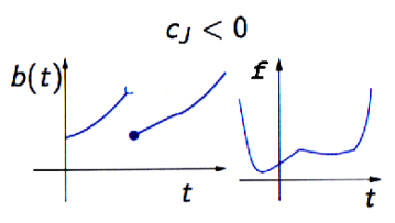
Figure 4: An exemplary function $b$ with one negative jump and its anti-derivative $f(x)=\int_{0}^{x}b(t)\,dt$

Further, for the sake of simplicity, we consider a function with one negative jump $c_{J}$ and estimate as follows:

$$c_{J}(x_{1}-x_{2})=c_{J}(x_{1}-x_{J})+c_{J}(x_{J}-x_{2})=c_{J}(x_{1}-x_{J})_{+}+c_{J}(x_{J}-x_{2})_{+}.$$ (24)

Using $x^{2}\geq(x-a)_{+}$ for any $a\geq\frac{1}{4}$, we get

$$(x_{1}-x_{2})^{2}\geq(x_{1}-x_{2}-\frac{1}{4})_{+}\geq(x_{1}-x_{2}-(x_{J}-x_{2}))_{+}=(x_{1}-x_{J})_{+}\quad\forall\,x_{2}\leq x_{J}-\frac{1}{4}$$

as well as

$$(x_{1}-x_{2})^{2}\geq(x_{1}-x_{2}-\frac{1}{4})_{+}\geq(x_{1}-x_{2}-(x_{1}-x_{J}))_{+}=(x_{J}-x_{2})_{+}\quad\forall\,x_{1}\geq x_{J}+\frac{1}{4}.$$

Hence, the condition (19) is fulfilled with $\alpha_{0}-2c_{J}>0$, but only for those $x_{1},x_{2}$ satisfying $x_{1}\geq x_{J}+\frac{1}{4}$ and $x_{2}\leq x_{J}-\frac{1}{4}$.

Let $h(t)$ be a Lipschitz continuous function with Lipschitz constant $c_{L}$. We include the negative jump $c^{J}$ at the point $t_{J}$ through the Heaviside function $\Theta$ by

$$b(t)=h(t)+c^{J}\Theta(t-t_{J})$$

and compute

$$f^{0}(t;d)=\left\{\begin{array}[]{ll}h(t)d,&\,\mbox{if}\;t<t_{J}\\[2.84544pt] h(t)d+c_{J}d,&\,\mbox{if}\;t>t_{J},\end{array}\right.\quad f^{0}(t_{J};d)=\left\{\begin{array}[]{ll}h(t_{J})d,&\,\mbox{if}\;d>0\\[2.84544pt] h(t_{J})d+c_{J}d,&\,\mbox{if}\;d\leq 0.\end{array}\right.$$

Hence, for any $t_{1},t_{2}<t_{J}$, we have

$$f^{0}(t_{1};t_{2}-t_{1}) +f^{0}(t_{2};t_{1}-t_{2})=h(t_{1})(t_{2}-t_{1})+h(t_{2})(t_{1}-t_{2})$$

$$= (h(t_{2})-h(t_{1}))(t_{1}-t_{2})\leq c_{L}(t_{1}-t_{2})^{2}.$$ (25)

Analogously, for any $t_{1},t_{2}>t_{J}$, we get

$$f^{0}(t_{1};t_{2}-t_{1})+f^{0}(t_{2};t_{1}-t_{2})= h(t_{1})(t_{2}-t_{1})+c_{J}(t_{2}-t_{1})+h(t_{2})(t_{1}-t_{2})$$

$$+c_{J}(t_{1}-t_{2})\leq c_{L}(t_{1}-t_{2})^{2}.$$

In both cases, the condition (20) is satisfied.
Let now $t_{1}<t_{J}\leq t_{2}$, then we have

$$f^{0}(t_{1};t_{2}-t_{1}) +f^{0}(t_{2};t_{1}-t_{2})=h(t_{1})(t_{2}-t_{1})+h(t_{2})(t_{1}-t_{2})+c_{J}(t_{1}-t_{2})$$

$$\quad\leq c_{L}(t_{1}-t_{2})^{2}+c_{J}(t_{1}-t_{2})\leq\alpha_{0}(t_{1}-t_{2})^{2}$$ (26)

for some $\alpha_{0}$ if and only if

$$\frac{c_{J}}{t_{1}-t_{2}}+c_{L}\leq\alpha_{0}.$$ (27)

Thus, we assume

$$c_{L}<\alpha_{0}\quad\mbox{and}\quad t_{1}\leq t_{J}-\frac{c_{J}}{c_{L}-\alpha_{0}},$$ (28)

which, since $t_{J}\leq t_{2}$, implies (27) immediately.

Based on the results presented in the Examples 1 and 2 we derive the following uniqueness result.

Theorem 5.2

Let $\mathbf{u}$ be a solution of the BIHVI problem $(\mathcal{P})$. Then $\mathbf{u}$ is unique if one of the following conditions holds:

• The jumps $c^{i}_{J}$ are non-negative and the Lipschitz constant $c_{L}$ satisfies $c_{L}<c_{P}$.

• The jump $c_{J}$ is negative, $c_{L}<c_{P}$ and ${u}_{n}(x)\leq t_{J}-\frac{1}{\tilde{c}}$ on $\Gamma_{C}$ for some positive $\tilde{c}$ such that $\tilde{c}<-\frac{c_{P}-c_{L}}{c_{J}}$.

Proof (b)  Let $\mathbf{u}\in\mathcal{V}$ be such that ${u}_{n}(x)\leq t_{J}-\frac{1}{\tilde{c}}$ on $\Gamma_{C}$ and $\mathbf{v}\in\mathcal{V}$ arbitrary. With $\alpha_{0}:=c_{L}-\tilde{c}\,c_{J}$, using (25) and (2), we obtain

$$\varphi(\mathbf{u},\mathbf{v}) +\varphi(\mathbf{v},\mathbf{u})=\int_{\Gamma_{C}}f^{0}(u_{n};v_{n}-u_{n})\,ds+\int_{\Gamma_{C}}f^{0}(v_{n};u_{n}-v_{n})\,ds$$

$$= \int_{\{s\in\Gamma_{C}\,:\,v_{n}(s)<t_{J}\}}f^{0}(u_{n};v_{n}-u_{n})\,ds+\int_{\{s\in\Gamma_{C}\,:\,v_{n}(s)\geq t_{J}\}}f^{0}(u_{n};v_{n}-u_{n})\,ds$$

$$+\int_{\{s\in\Gamma_{C}\,:\,v_{n}(s)<t_{J}\}}f^{0}(v_{n};u_{n}-v_{n})\,ds+\int_{\{s\in\Gamma_{C}\,:\,v_{n}(s)\geq t_{J}\}}f^{0}(v_{n};u_{n}-v_{n})\,ds$$

$$\leq \int_{\{s\in\Gamma_{C}\,:\,v_{n}(s)<t_{J}\}}c_{L}(u_{n}-v_{n})^{2}\,ds+\int_{\{s\in\Gamma_{C}\,:\,v_{n}(s)\geq t_{J}\}}\alpha_{0}(u_{n}-v_{n})^{2}\,ds$$

$$\leq \max\{c_{L},\alpha_{0}\}\left\|u_{n}-v_{n}\right\|^{2}_{L^{2}(\Gamma_{C})}\leq\alpha_{0}\left\|\mathbf{u}-\mathbf{v}\right\|^{2}_{\mathcal{V}}.$$ (29)

Further, we assume that $\mathbf{\tilde{u}}\in\mathcal{V}$ is another solution of $(\mathcal{P})$. Following the proof of Theorem 5.1, in virtue of $\alpha_{0}=c_{L}-\tilde{c}\,c_{J}<c_{p}$ and (29) with $\mathbf{v}:=\mathbf{\tilde{u}}$, we obtain a contradiction. ∎

Remark 3

We note that our uniqueness result is more general then the result in (Nesemann, , Theorem 7), which demands $\tilde{c}=4$.

5.2 Uniqueness of the regularized problem

Assumption 3

Assume that the assumption (19) is satisfied for the regularization function, i.e. there exists a constant $\alpha_{0}\geq 0$ (in general depending on $\varepsilon>0$) such that

$$\left(S_{x}(x_{1},\varepsilon)-S_{x}(x_{2},\varepsilon)\right)(x_{1}-x_{2})\geq-\alpha_{0}|x_{1}-x_{2}|^{2}\quad\forall\,x_{1},x_{2}\in\mathbb{R}.$$ (30)

Hence, for any $\mathbf{u},\mathbf{v}\in\mathcal{V}$, we have

$$\langle DJ_{\varepsilon}(\mathbf{u})-DJ_{\varepsilon}(\mathbf{v}),\mathbf{v}-\mathbf{u}\rangle_{\Gamma_{C}} =\int_{\Gamma_{C}}\left(S_{x}({u}_{n}(s),\varepsilon)-S_{x}({v}_{n}(s),\varepsilon)\right)(v_{n}(s)-{u}_{n}(s))\,ds$$

$$\leq\alpha_{0}\|{u}_{n}-{v}_{n}\|^{2}_{L^{2}(\Gamma_{C})}\leq\alpha_{0}\|\mathbf{u}-\mathbf{v}\|^{2}_{\mathcal{V}}.$$ (31)

Due to Theorem 5.1, we have the following uniqueness result for the regularized problem.

Theorem 5.3

Under the assumption (30) with $\alpha_{0}<c_{p}$, there exists a unique solution to the regularized problem $(\mathcal{P}_{\varepsilon})$, which depends Lipschitz continuously on the right hand side $\mathbf{F}\in\mathcal{V}^{*}$.

One of the most interesting question is, which classes of smoothing functions preserve the property of unique solvability of the original problem as $\varepsilon\to 0^{+}$. As the next example shows, this is the case for the smoothing function (8) relevant to our computation. In particular, we show that the constant $\alpha_{0}$ in (30) does not depend on $\varepsilon$.

Example 3

In view of our application to contact problems with nonmonotone laws in the boundary conditions, we consider $f(x)=\max\{g_{1}(x),g_{2}(x)\}$ with $g_{i}(x)=\frac{a_{i}}{2}x^{2}+c_{i}x+d_{i}.$ We use the smoothing function (8) as a regularization of $f$. The corresponding approximation of $\partial f$ is given by

$$S_{x}(x,\varepsilon)=\left\{\begin{array}[]{ll}g_{1}^{\prime}(x)&\mbox{if}\,\;g_{2}(x)-g_{1}(x)\leq-\frac{\varepsilon}{2}\\[2.84544pt] \lambda_{1}g_{1}^{\prime}(x)+\lambda_{2}g_{2}^{\prime}(x)&\mbox{if}\,\;\left|g_{1}(x)-g_{2}(x)\right|<\frac{\varepsilon}{2}\\[2.84544pt] g_{2}^{\prime}(x)&\mbox{if}\,\;g_{2}(x)-g_{1}(x)\geq\frac{\varepsilon}{2},\end{array}\right.$$

where

$$\lambda_{2}=\frac{1}{\varepsilon}(g_{2}(x)-g_{1}(x))+\frac{1}{2},\quad\lambda_{1}=1-\lambda_{2}.$$

We need to consider only the region $I_{\varepsilon}:=\{x\in\mathbb{R}\,:\,|g_{1}(x)-g_{2}(x)|<\frac{\varepsilon}{2}\}$, where $f$ is actually approximated. Otherwise, the condition (30) is automatically satisfied.
Let $x_{i}\in I_{\varepsilon},\;i=1,2$. Setting $g(x):=g_{1}(x)-g_{2}(x)$, we introduce

$$\lambda_{2}^{i}=\frac{1}{\varepsilon}(g_{2}(x_{i})-g_{1}(x_{i}))=-\frac{1}{\varepsilon}g(x_{i})\;\mbox{and}\;\lambda_{1}^{i}=1-\lambda_{2}^{i},\;i=1,2.$$

Hence,

$$\lambda_{1}^{1}-\lambda_{1}^{2}=\lambda_{2}^{2}-\lambda_{2}^{1}=\frac{1}{\varepsilon}(g(x_{1})-g(x_{2}))$$ (32)

and thus,

$$S_{x}(x_{1},\varepsilon)-S_{x}(x_{2},\varepsilon) =\lambda_{1}^{1}(a_{1}x_{1}+c_{1})+\lambda_{2}^{1}(a_{2}x_{1}+c_{2})-\lambda_{1}^{2}(a_{1}x_{2}+c_{1})$$

$$\quad-\lambda_{2}^{2}(a_{2}x_{2}+c_{2})$$

$$=a_{1}\lambda_{1}^{1}(x_{1}-x_{2})+a_{2}\lambda_{2}^{1}(x_{1}-x_{2})+(\lambda_{1}^{1}-\lambda_{1}^{2})(a_{1}x_{2}+c_{1})$$

$$\quad+(\lambda_{2}^{1}-\lambda_{2}^{2})(a_{2}x_{2}+c_{2})$$

$$=\left(a_{1}\lambda_{1}^{1}+a_{2}\lambda_{2}^{1}\right)(x_{1}-x_{2})+(\lambda_{1}^{1}-\lambda_{1}^{2})(g_{1}^{\prime}(x_{2})-g_{2}^{\prime}(x_{2}))$$

$$=\left(a_{1}\lambda_{1}^{1}+a_{2}\lambda_{2}^{1}\right)(x_{1}-x_{2})+(\lambda_{1}^{1}-\lambda_{1}^{2})g^{\prime}(x_{2}).$$ (33)

Similarly to (33), we find that

$$S_{x}(x_{1},\varepsilon)-S_{x}(x_{2},\varepsilon)=\left(a_{1}\lambda_{1}^{2}+a_{2}\lambda_{2}^{2}\right)(x_{1}-x_{2})+(\lambda_{1}^{1}-\lambda_{1}^{2})g^{\prime}(x_{1}).$$ (34)

Summing now (33) and (34), we get

$$2\left(S_{x}(x_{1},\varepsilon)-S_{x}(x_{2},\varepsilon)\right) =(a_{1}\lambda_{1}^{1}+a_{2}\lambda_{2}^{1}+a_{1}\lambda_{1}^{2}+a_{2}\lambda_{2}^{2})(x_{1}-x_{2})$$

$$\quad+(\lambda_{1}^{1}-\lambda_{1}^{2})(g^{\prime}(x_{1})+g^{\prime}(x_{2})).$$ (35)

From (32), using the structure of $g_{1}$ and $g_{2}$, we find that

$$\lambda_{1}^{1}-\lambda_{1}^{2} =\frac{1}{\varepsilon}(g(x_{1})-g(x_{2}))=\frac{1}{\varepsilon}\left(\frac{a_{1}-a_{2}}{2}(x_{1}^{2}-x_{2}^{2})+(c_{1}-c_{2})(x_{1}-x_{2})\right)$$

$$=\frac{1}{\varepsilon}(x_{1}-x_{2})\left(\frac{a_{1}-a_{2}}{2}x_{1}+\frac{c_{1}-c_{2}}{2}+\frac{a_{1}-a_{2}}{2}x_{2}+\frac{c_{1}-c_{2}}{2}\right)$$

$$=\frac{1}{2\varepsilon}(x_{1}-x_{2})(g^{\prime}(x_{1})+g^{\prime}(x_{2})).$$ (36)

Hence,

$$2\left(S_{x}(x_{1},\varepsilon)-S_{x}(x_{2},\varepsilon)\right)(x_{1}-x_{2})\geq(a_{1}\lambda_{1}^{1}+a_{2}\lambda_{2}^{1}+a_{1}\lambda_{1}^{2}+a_{2}\lambda_{2}^{2})(x_{1}-x_{2})^{2}$$

$$\quad=(a_{1}(1-\lambda_{2}^{1})+a_{2}\lambda_{2}^{1}+a_{1}(1-\lambda_{2}^{2})+a_{2}\lambda_{2}^{2})(x_{1}-x_{2})^{2}$$

$$\quad\geq(-|a_{1}||(1-\lambda_{2}^{1})|-|a_{2}||\lambda_{2}^{1}|-|a_{1}||(1-\lambda_{2}^{2})|-|a_{2}||\lambda_{2}^{2}|)(x_{1}-x_{2})^{2}$$

$$\quad\geq-\max\{|a_{1}|,|a_{2}|\}(|(1-\lambda_{2}^{1})|+|\lambda_{2}^{1}|+|(1-\lambda_{2}^{2})|+|\lambda_{2}^{2}|)(x_{1}-x_{2})^{2}$$

$$\quad\geq-\max\{|a_{1}|,|a_{2}|\}(3/2+1/2+3/2+1/2)(x_{1}-x_{2})^{2}$$

$$\quad=-4\max\{|a_{1}|,|a_{2}|\}(x_{1}-x_{2})^{2}$$

and consequently, (30) is satisfied with $\alpha_{0}=2\max\{|a_{1}|,|a_{2}|\}$.

Remark 4

If we use (8) as a smoothing approximation for the maximum (resp. minimum) function of several quadratic functions $a_{i}x^{2}+c_{i}x+d_{i}$, then (30) is satisfied and, therefore, the regularized problem is always uniquely solvable if all $|a_{i}|$ are sufficiently small. Since the constant $\alpha_{0}$ does not depend on $\varepsilon$, the property of uniqueness is preserved as $\varepsilon\to 0^{+}$.

6 Discretization with boundary elements

To avoid domain approximation, let $\Omega\subset\mathbb{R}^{d}$, $d=2,3$, also be a polygonal domain. Let $\mathcal{T}_{h}$ be a sufficiently fine finite element mesh of the boundary $\Gamma$ respecting the decomposition of $\Gamma$ into $\Gamma_{D}$, $\Gamma_{N}$ and $\Gamma_{C}$, $p=(p_{T})_{T\in\mathcal{T}_{h}}$ a polynomial degree distribution over $\mathcal{T}_{h}$, $\mathbb{P}_{p_{T}}(\hat{T})$ the space of polynomials of order $p_{T}$ on the reference element $\hat{T}$, and $\Psi_{T}:\hat{T}\rightarrow T\in\mathcal{T}_{h}$ a bijective, (bi)-linear transformation. In 2D, $\hat{T}$ is the interval $[-1,1]$, whereas in 3D it is the reference square $[-1,1]^{2}$. Let $\Sigma_{T,hp}$ be the set of all affinely transformed (tensor product based) Gauss-Lobatto nodes on the element $T$ of the partition $\mathcal{T}_{h}$ of $\Gamma$, corresponding to the polynomial degree $p_{T}$, and set $\displaystyle\Sigma_{hp}:=\displaystyle\bigcup_{T\in\mathcal{T}_{h}|_{\Gamma_{C}}}\Sigma_{T,hp}$, see krebs2007p ; MS-1 ; gwinner2013hp . Furthermore, we assume in this section that $g\in C^{0}(\overline{\Gamma_{C}})$ to allow point evaluation.
For the discretization of the displacement $\mathbf{u}$ we use

$$\mathcal{V}_{hp} =\{\mathbf{v_{hp}}\in\mathbf{C}^{0}(\Gamma)\,:\,\mathbf{v_{hp}}|_{T}\circ\Psi_{T}\in[\mathbb{P}_{p_{T}}(\hat{T})]^{d}\quad\forall\,T\in\mathcal{T}_{h},\;\mathbf{v_{hp}}=0\;\mbox{on}\;\overline{\Gamma_{D}}\},$$

$$\mathcal{K}_{hp}^{\Gamma} =\{\mathbf{v_{hp}}\in\mathcal{V}_{hp}\,:\,(\mathbf{v_{hp}}\cdot\mathbf{n})(P_{i})\leq g(P_{i})\quad\forall\,P_{i}\in\Sigma_{hp}\}.$$

In general $\mathcal{K}_{hp}^{\Gamma}\not\subseteq\mathcal{K}^{\Gamma}$. For the approximation of the Poincaré-Steklov operator, namely $V^{-1}$, we need the space

$$\mathcal{W}_{hp}=\{\psi_{hp}\in\mathbf{L}^{2}(\Gamma)\,:\,\psi_{hp}|_{T}\circ\Psi_{T}\in[\mathbb{P}_{p_{T}-1}(\hat{T})]^{d}\quad\forall\,T\in\mathcal{T}_{h}\}\subset\mathbf{H}^{-1/2}(\Gamma).$$

For more details on the approximation techniques based on boundary element method see e.g. ccjg ; Co-1 ; CoSt ; Gu ; GS-1 ; Ha ; MS-1 ; MS-2 ; SlSp . Let $\{\phi_{i}\}_{i=1}^{N_{D}}$ and $\{\psi_{j}\}_{j=1}^{N_{N}}$ be a bases of $\mathcal{V}_{hp}$ and $\mathcal{W}_{hp}$, respectively. Then, the boundary matrices are given by

$$(V_{hp})_{j,i} =\langle V\psi_{i},\psi_{j}\rangle,\quad(K_{hp})_{j,i}=\langle K\phi_{i},\psi_{j}\rangle,$$

$$(W_{hp})_{j,i} =\langle W\phi_{i},\phi_{j}\rangle,\quad(I_{hp})_{j,i}=\langle\phi_{i},\psi_{j}\rangle$$

and, therewith, the approximation of the Galerkin matrix is

$${P}_{hp}=W_{hp}+\left(K_{hp}+\frac{1}{2}I_{hp}\right)^{\top}V^{-1}_{hp}\left(K_{hp}+\frac{1}{2}I_{hp}\right).$$

With the canonical embeddings

$$i_{hp}:\mathcal{W}_{hp}\hookrightarrow\mathbf{H}^{-1/2}(\Gamma)\,,\qquad j_{hp}:\mathcal{V}_{hp}\hookrightarrow\mathbf{H}^{1/2}(\Gamma)$$

and their duals $i_{hp}^{*}$ and $j_{hp}^{*}$, the discrete Poincaré-Steklov operator $P_{hp}:\mathcal{V}_{hp}\to\mathcal{V}_{hp}^{*}$ can be also represented by

$$P_{hp}=j_{hp}^{*}Wj_{hp}+j_{hp}^{*}\left(K^{\prime}+\frac{1}{2}I\right)i_{hp}(i_{hp}^{*}Vi_{hp})^{-1}i_{hp}^{*}\left(K+\frac{1}{2}I\right)j_{hp}.$$

According to cc , see e.g. Banz2015Stab for the $hp$-version, this functional is well-defined and satisfies

$$\exists\,c>0:\quad\langle P_{hp}\mathbf{v}_{hp},\mathbf{v}_{hp}\rangle_{\Gamma_{0}}\geq c\|\mathbf{v}_{hp}\|_{\tilde{\mathbf{H}}^{1/2}(\Gamma_{0})}\qquad\forall\,\mathbf{v}_{hp}\in\mathcal{V}_{hp}$$ (37)

if $\min\{h,p^{-1}\}$ is sufficiently small. Further, we consider the operator $E_{hp}:\mathbf{H}^{1/2}(\Gamma)\to\mathbf{H}^{-1/2}(\Gamma)$, reflecting the consistency error in the discretization of the Poincaré-Steklov operator $P$, defined by

$$E_{hp}:=P-P_{hp}=\left(\frac{1}{2}I+K^{\prime}\right)\left(V^{-1}-i_{hp}(i_{hp}^{*}Vi_{hp})^{-1}i_{hp}^{*}\right)\left(\frac{1}{2}I+K\right).$$

From MS-1 (see also cc ), the operator $E_{hp}$ is bounded and there exists a constant $c>0$ such that

$$\|E_{hp}\mathbf{v}\|_{\mathbf{H}^{-1/2}(\Gamma)}\leq c\,\displaystyle\inf_{{\psi_{hp}}\in\mathcal{W}_{hp}}\|V^{-1}(I+K)\mathbf{v}-{\psi_{hp}}\|_{\mathbf{H}^{-1/2}(\Gamma)}\quad\forall\,\mathbf{v}\in\mathbf{H}^{1/2}(\Gamma).$$

Now, we turn to the discretization of the regularized problem $(\mathcal{P}_{\varepsilon})$. The discretized regularized problem ($\mathcal{P}_{\varepsilon,hp}$) is: Find $\mathbf{u}^{\varepsilon}_{hp}\in\mathcal{K}^{\Gamma}_{hp}$ such that for all $\forall\,\mathbf{v}_{hp}\in\mathcal{K}_{hp}^{\Gamma}$

$$\langle{P}_{hp}\mathbf{u}^{\varepsilon}_{hp},\mathbf{v}_{hp}-\mathbf{u}^{\varepsilon}_{hp}\rangle_{\Gamma_{0}}+\langle DJ_{\varepsilon}(\mathbf{u}^{\varepsilon}_{hp}),\mathbf{v}_{hp}-\mathbf{u}^{\varepsilon}_{hp}\rangle_{\Gamma_{C}}\geq\langle\mathbf{F},\mathbf{v}_{hp}-\mathbf{u}^{\varepsilon}_{hp}\rangle_{\Gamma_{0}}.$$ (38)

The convergence result for the $hp$-solution $\mathbf{u}^{\varepsilon}_{hp}$ of ($\mathcal{P}_{\varepsilon,hp}$) is due to the following abstract approximation result from Gw_Ov .

Let $\mathcal{K}$ be a closed, convex nonempty subset of a reflexive Banach space $X$ and $VI(\psi,f,\mathcal{K})$ be the pseudo-monotone variational inequality: Find $u\in\mathcal{K}$ such that $\psi(u,v)\geq\langle f,v-u\rangle\,\forall\,v\in\mathcal{K}.$ Let $T$ be a directed set. We introduce the family $\{\mathcal{K}_{t}\}_{t\in T}$ of nonempty, closed and convex sets and admit the following hypotheses:

•

(H1) If $\{v_{t^{\prime}}\}_{t^{\prime}\in T^{\prime}}$ weakly converges to $v$ in $X$, $v_{t^{\prime}}\in\mathcal{K}_{t^{\prime}}~{}(t^{\prime}\in T^{\prime})$ for a subnet $\{\mathcal{K}_{t^{\prime}}\}_{t^{\prime}\in T^{\prime}}$ of the net $\{\mathcal{K}_{t}\}_{t\in T}$, then $v\in\mathcal{K}$.

•

(H2) For any $v\in\mathcal{K}$ and any $t\in T$ there exists $v_{t}\in\mathcal{K}_{t}$ such that $v_{t}\to v$ in $X$.

•

(H3) $\psi_{t}$ is pseudomonotone for any $t\in T$.

•

(H4) $f_{t}\to f$ in $V^{\ast}$.

•

(H5) For any nets $\{u_{t}\}$ and $\{v_{t}\}$ such that $u_{t}\in\mathcal{K}_{t}$, $v_{t}\in\mathcal{K}_{t}$, $u_{t}\rightharpoonup u$, and $v_{t}\to v$ in $X$ it follows that

$${\liminf_{t\in T}}\,~{}\psi_{t}(u_{t},v_{t})\leq\psi(u,v)\,.$$

•

(H6) There exist constants $c>0$, $d$, $d_{0}\in\mathbb{R}$ and $\alpha>1$ (independent of $t\in T$) such that for some $w_{t}\in\mathcal{K}_{t}$ with $w_{t}\to w$ there holds

$$-\psi_{t}(u_{t},w_{t})\geq c\|u_{t}\|^{\alpha}_{V}+d\|u_{t}\|_{V}+d_{0},\quad\forall\,u_{t}\in\mathcal{K}_{t},\;\forall\,t\in T\,.$$

Theorem 6.1

Under the hypotheses $(H1)$-$(H6)$, there exists a solution to the problem $VI(\psi_{t},f_{t},\mathcal{K}_{t})$. Moreover, the family $\{u_{t}\}$ of solutions to the problem $VI(\psi_{t},f_{t},\mathcal{K}_{t})$ is bounded in $X$ and there exists a subnet of $\{u_{t}\}$ that converges weakly in $X$ to a solution of the problem $VI(\psi,f,\mathcal{K})$.

The hypotheses (H1) and (H2) are due to Glowinski Gl and describe the Mosco convergence At of the family $\mathcal{K}_{t}$ to $\mathcal{K}$, whereas $f_{t}$ in (H4) is a standard approximation of the linear functional $f$, for example, by numerical integration. The hypotheses (H5)-(H6) have been verified in Ovcharova2015 .

We apply Theorem 6.1 with $t=(\varepsilon,h,p)$ and show convergence for $\varepsilon\to 0^{+}$, and either $p\to\infty$ or $h\to 0$. We emphasize that in fact the weak convergence of $\{\mathbf{u}^{\varepsilon}_{hp}\}$ to $\mathbf{u}$ in $\mathbf{H}^{1/2}(\Gamma)$ can be replaced by the strong one. The complete proof of this result for the $h$-version of BEM can be found in Ovcharova2015 .

7 A-priori error estimate for the regularized problem

In this section we provide an a-priori error estimate for the $hp$-approximate solution $\mathbf{u}^{\varepsilon}_{hp}$ of the regularized boundary variational problem $(\mathcal{P}_{\varepsilon})$ under the regularity assumptions of MS-1 for Signorini contact, i.e. $\mathbf{u}_{\varepsilon}\in\mathbf{H}^{3/2}(\Gamma)$ and $g\in H^{3/2}(\Gamma_{C})$. For our more general variational problem $(\mathcal{P}_{\varepsilon})$ we arrive at the same convergence order of $\mathcal{O}(h^{1/4}p^{-1/4})$ as Maischak and Stephan in MS-1 . To this end, we present the following Céa-Falk approximation lemma for the regularized problem $(\mathcal{P}_{\varepsilon})$.

Lemma 3

Let $\mathbf{u}_{\varepsilon}\in\mathcal{K}^{\Gamma}$ be the solution of the problem $(\mathcal{P}_{\varepsilon})$ and let $\mathbf{u}^{\varepsilon}_{hp}\in\mathcal{K}_{hp}^{\Gamma}$ be the solution of the problem $(\mathcal{P}_{\varepsilon,hp})$. Assume that $\alpha_{0}<c_{p}$, $\mathbf{u}_{\varepsilon}$ $\in\mathbf{H}^{3/2}(\Gamma)$, $g\in H^{3/2}(\Gamma_{C})$ and $P\mathbf{u}_{\varepsilon}-\mathbf{F}\in\mathbf{L}^{2}(\Gamma)$. Then there exists a constant $c=c(\mathbf{u}_{\varepsilon},g,\mathbf{f},\mathbf{t})>0$, but independent of $h$ and $p$ such that

$$c \|\mathbf{u}_{\varepsilon}-\mathbf{u}^{\varepsilon}_{hp}\|^{2}_{\mathbf{H}^{1/2}(\Gamma)}\leq\|E_{hp}(\mathbf{u}_{\varepsilon})\|^{2}_{\mathbf{H}^{-1/2}(\Gamma)}$$

$$\quad+\inf_{v\in\mathcal{K}^{\Gamma}}\{\|P\mathbf{u}_{\varepsilon}-\mathbf{F}\|_{\mathbf{L}^{2}(\Gamma)}\|\mathbf{u}^{\varepsilon}_{hp}-\mathbf{v}\|_{\mathbf{L}^{2}(\Gamma)}+\langle DJ_{\varepsilon}(\mathbf{u}_{\varepsilon}),\mathbf{v}-\mathbf{u}^{\varepsilon}_{hp}\rangle_{\Gamma_{C}}\}$$

$$\quad+\inf_{v_{hp}\in\mathcal{K}_{hp}^{\Gamma}}\left\{\|\mathbf{u}_{\varepsilon}-\mathbf{v}_{hp}\|_{\mathbf{H}^{1/2}(\Gamma)}^{2}+\|P\mathbf{u}_{\varepsilon}-\mathbf{F}\|_{\mathbf{L}^{2}(\Gamma)}\|\mathbf{u}_{\varepsilon}-\mathbf{v}_{hp}\|_{\mathbf{L}^{2}(\Gamma)}\right.$$

$$\quad\left.+\langle DJ_{\varepsilon}(\mathbf{u}^{\varepsilon}_{hp}),\mathbf{v}_{hp}-\mathbf{u}_{\varepsilon}\rangle_{\Gamma_{C}}\right\}.$$

Proof Using the definitions of $(\mathcal{P}_{\varepsilon})$ and $(\mathcal{P}_{\varepsilon,hp})$, and estimates similar to (MS-1, , Theorem 3), we obtain for all $v\in\mathcal{K}^{\Gamma}$, $v_{hp}\in\mathcal{K}_{hp}^{\Gamma}$

$$c_{P} \|\mathbf{u}_{\varepsilon}-\mathbf{u}^{\varepsilon}_{hp}\|^{2}_{\mathbf{H}^{1/2}(\Gamma)}\leq\|E_{hp}(\mathbf{u}_{\varepsilon})\|^{2}_{\mathbf{H}^{-1/2}(\Gamma)}+\|\mathbf{u}_{\varepsilon}-\mathbf{v}_{hp}\|_{\mathbf{H}^{1/2}(\Gamma)}^{2}$$

$$+\|P\mathbf{u}_{\varepsilon}-\mathbf{F}\|_{\mathbf{L}^{2}(\Gamma)}\left(\|\mathbf{u}_{\varepsilon}-\mathbf{v}_{hp}\|_{\mathbf{L}^{2}(\Gamma)}+\|\mathbf{u}^{\varepsilon}_{hp}-\mathbf{v}\|_{\mathbf{L}^{2}(\Gamma)}\right)+{\rm D},$$

where we abbreviate

$${\rm D}=\langle DJ_{\varepsilon}(\mathbf{u}_{\varepsilon}),\mathbf{v}-\mathbf{u}_{\varepsilon}\rangle_{\Gamma_{C}}+\langle DJ_{\varepsilon}(\mathbf{u}^{\varepsilon}_{hp}),\mathbf{v}_{hp}-\mathbf{u}^{\varepsilon}_{hp}\rangle_{\Gamma_{C}}.$$

To bound the term ${\rm D}$, we use (31) and estimate as follows:

$${\rm D} =\langle DJ_{\varepsilon}(\mathbf{u}_{\varepsilon}),\mathbf{v}-\mathbf{u}^{\varepsilon}_{hp}\rangle_{\Gamma_{C}}+\langle DJ_{\varepsilon}(\mathbf{u}^{\varepsilon}_{hp}),\mathbf{v}_{hp}-\mathbf{u}_{\varepsilon}\rangle_{\Gamma_{C}}$$

$$\quad+\langle DJ_{\varepsilon}(\mathbf{u}_{\varepsilon})-DJ_{\varepsilon}(\mathbf{u}^{\varepsilon}_{hp}),\mathbf{u}^{\varepsilon}_{hp}-\mathbf{u}_{\varepsilon}\rangle_{\Gamma_{C}}$$

$$\leq\langle DJ_{\varepsilon}(\mathbf{u}_{\varepsilon}),\mathbf{v}-\mathbf{u}^{\varepsilon}_{hp}\rangle_{\Gamma_{C}}+\langle DJ_{\varepsilon}(\mathbf{u}^{\varepsilon}_{hp}),\mathbf{v}_{hp}-\mathbf{u}_{\varepsilon}\rangle_{\Gamma_{C}}+\alpha_{0}\|\mathbf{u}_{\varepsilon}-\mathbf{u}^{\varepsilon}_{hp}\|^{2}_{\mathcal{V}}.$$

Therefore, since $\alpha_{0}<c_{P}$, see Theorem 5.3, we obtain the assertion. ∎

Theorem 7.1

Let $\mathbf{u}_{\varepsilon}\in\mathcal{K}^{\Gamma}$ be the solution of the problem $(\mathcal{P}_{\varepsilon})$ and let $\mathbf{u}^{\varepsilon}_{hp}\in\mathcal{K}_{hp}^{\Gamma}$ be the solution of the problem $(\mathcal{P}_{\varepsilon,hp})$. Assume that $\alpha_{0}<c_{p}$, $\mathbf{u}_{\varepsilon}$ $\in\mathbf{H}^{3/2}(\Gamma)$, $g\in H^{3/2}(\Gamma_{C})$ and $P\mathbf{u}_{\varepsilon}-\mathbf{F}\in\mathbf{L}^{2}(\Gamma)$. Then there exists a constant $c=c(\mathbf{u}_{\varepsilon},g,\mathbf{f},\mathbf{t})>0$, but independent of $h$ and $p$ such that

$$\|\mathbf{u}_{\varepsilon}-\mathbf{u}^{\varepsilon}_{hp}\|_{\mathbf{H}^{1/2}(\Gamma)}\leq ch^{1/4}p^{-1/4}.$$ (39)

Proof Taking into account the estimates obtained by Maischak and Stephan in (MS-1, , Theorem 3) for the consistency error, the approximation error, and for $\|E_{hp}{\mathbf{u}}\|_{\mathbf{H}^{-1/2}(\Gamma)}$, we only need to estimate

$$\inf\{\langle DJ_{\varepsilon}(\mathbf{u}_{\varepsilon}),\mathbf{v}-\mathbf{u}^{\varepsilon}_{hp}\rangle_{\Gamma_{C}}\,:\,\mathbf{v}\in\mathcal{K}^{\Gamma}\}$$ (40)

and

$$\inf\{\langle DJ_{\varepsilon}(\mathbf{u}^{\varepsilon}_{hp}),\mathbf{v}_{hp}-\mathbf{u}_{\varepsilon}\rangle_{\Gamma_{C}}\,:\,\mathbf{v}_{hp}\in\mathcal{K}_{hp}^{\Gamma}\}.$$ (41)

To estimate (41) we take $\mathbf{v}_{hp}:=I_{hp}\mathbf{u}_{\varepsilon}\in\mathcal{K}_{hp}^{\Gamma}$, the interpolate of $\mathbf{u}_{\varepsilon}\in\mathbf{H}^{3/2}(\Gamma)\subset C^{0}(\Gamma)$. From (14a),

$$\langle DJ_{\varepsilon}(\mathbf{u}^{\varepsilon}_{hp}),\mathbf{v}_{hp}-\mathbf{u}_{\varepsilon}\rangle_{\Gamma_{C}} =\int_{\Gamma_{C}}S_{x}(u^{\varepsilon}_{hp,n},\varepsilon)(v_{hp,n}-u_{\varepsilon,n})\,ds$$

$$\leq c\left(1+\|u^{\varepsilon}_{hp,n}\|_{L^{2}(\Gamma_{C})}\right)\|u_{\varepsilon,n}-v_{hp,n}\|_{L^{2}(\Gamma_{C})}.$$ (42)

By (Bernardi, , Theorems 4.2 and 4.5) and by the real interpolation between $H^{1}(\Gamma)$ and $L^{2}(\Gamma)$ there exists a constant $C_{1}>0$ such that

$$\|u_{\varepsilon,n}-v_{hp,n}\|_{H^{1/2}(\Gamma)}\leq C_{1}h^{1}p^{-1}\,\|\mathbf{u}_{\varepsilon}\|_{H^{3/2}(\Gamma)}.$$ (43)

To estimate (40) similarly as MS-1 we define $\mathbf{v}^{*}\in\mathcal{K}^{\Gamma}\cap\mathbf{H}^{1}(\Gamma)$ by

$$\mathbf{v}^{*}:=\left\{\begin{array}[]{lc}\mathbf{u}^{\varepsilon}_{hp,t}+[g+\inf\{u^{\varepsilon}_{hp,n}-g_{hp},0\}]\mathbf{n}&\mbox{on}\;\Gamma_{C}\\ 0&\mbox{on}\;\Gamma_{D}\\ \gamma_{N}\mathbf{u}^{\varepsilon}_{hp}&\mbox{on}\;\Gamma_{N},\end{array}\right.$$

where $g_{hp}:=I_{hp}g$ is the interpolate of the gap function $g$, and $\gamma_{N}$ is the trace map onto $\Gamma_{N}$.
Analogously to (42), we have

$$\langle DJ_{\varepsilon}(\mathbf{u}_{\varepsilon}),\mathbf{v}^{*}-\mathbf{u}^{\varepsilon}_{hp}\rangle_{\Gamma_{C}} =\int_{\Gamma_{C}}S_{x}(u_{\varepsilon,n},\varepsilon)(v^{*}_{n}-u^{\varepsilon}_{hp,n})\,ds$$

$$\leq c\left(1+\|u_{\varepsilon,n}\|_{L^{2}(\Gamma_{C})}\right)\|v^{*}_{n}-u^{\varepsilon}_{hp,n}\|_{L^{2}(\Gamma_{C})}.$$ (44)

The elaborate analysis in MS-1 , see the proof of Theorem 3, estimates (31) - (33), gives

$$\|v^{*}_{n}-u^{\varepsilon}_{hp,n}\|_{L^{2}(\Gamma_{C})}\leq C_{2}h^{1/2}p^{-1/2}\left(\|g\|_{H^{1/2}(\Gamma_{C})}+\|\mathbf{u}^{\varepsilon}_{hp}\|_{H^{1/2}(\Gamma_{C})}\right).$$ (45)

Finally, combining the error estimates for the interpolation (43) and the consistency (45) with (42) and (44), respectively, and taking into account the boundedness of $\|\mathbf{u}^{\varepsilon}_{hp}\|$ in $H^{1/2}(\Gamma_{C})$ (see Theorem 6.1), we prove the wished bound for (40) and (41). ∎

Remark 5

Let $\mathbf{u}\in\mathcal{K}^{\Gamma}$ be the solution of the problem $(\mathcal{P})$ and $\mathbf{u}_{\varepsilon}\in\mathcal{K}^{\Gamma}$ be the solution of the problem $(\mathcal{P}_{\varepsilon})$. Taking $\mathbf{v}=\mathbf{u}_{\varepsilon}$ in (5) and $\mathbf{v}=\mathbf{u}$ in (15), and adding the two resulting inequalities yields

$$\langle P\mathbf{u}-P\mathbf{u}_{\varepsilon},\mathbf{u}_{\varepsilon}-\mathbf{u}\rangle_{\Gamma_{0}}+\varphi(\mathbf{u},\mathbf{u}_{\varepsilon})+\varphi_{\varepsilon}(\mathbf{u}_{\varepsilon},\mathbf{u})\geq 0.$$

Hence,

$$c_{P}\|\mathbf{u}_{\varepsilon}-\mathbf{u}\|^{2}_{\mathcal{V}}\leq\langle P\mathbf{u}_{\varepsilon}-P\mathbf{u},\mathbf{u}_{\varepsilon}-\mathbf{u}\rangle_{\Gamma_{0}}\leq\varphi(\mathbf{u},\mathbf{u}_{\varepsilon})+\varphi_{\varepsilon}(\mathbf{u}_{\varepsilon},\mathbf{u}).$$

We emphasize that, in general, the functional $\varphi_{\varepsilon}$ does not approximate the functional $\varphi$ arbitrarily close as $\varepsilon\to 0^{+}$. Nevertheless, we have convergence of the sequence $\{\mathbf{u}_{\varepsilon}\}$ of the solutions of the regularized problem ($\mathcal{P}_{\varepsilon}$) to the solution $\mathbf{u}$ of the boundary hemivariational problem ($\mathcal{P}$). In particular, for any $\mathbf{v}_{\varepsilon}\rightharpoonup\mathbf{v}$ it holds

$$\limsup_{\varepsilon\to 0}\,\varphi_{\varepsilon}(\mathbf{v}_{\varepsilon},\mathbf{v})\leq\varphi(\mathbf{v},\mathbf{v})\quad\forall\mathbf{v}\in\mathcal{K}^{\Gamma},$$

which according to Theorem 6.1 is a sufficient condition for convergence.
However, for convergence rates in $\varepsilon$,

$$\varphi(\mathbf{u},\mathbf{u}_{\varepsilon})+\varphi_{\varepsilon}(\mathbf{u}_{\varepsilon},\mathbf{u})\leq c\,\varepsilon^{\beta}\|\mathbf{u}_{\varepsilon}-\mathbf{u}\|_{\mathcal{V}}$$

for some positive constants $c$ and $\beta$ is needed. An estimate of this form can be found in Ovcharova2012 for the approximation of the absolute value function.

8 A-posteriori error estimate for the regularized problem

To be able to split the approximation error into the discretization error of a simpler variational equation and contributions arising from the constraints on $\Gamma_{C}$ we introduce the regularized mixed formulation (46a)-(46b), which is equivalent to the regularized problem $(\mathcal{P}_{\varepsilon})$.
Find $(\mathbf{u}^{\varepsilon},\lambda^{\varepsilon})\in\mathcal{V}\times M(\mathbf{u}^{\varepsilon})$ such that

$$\left\langle P\mathbf{u}^{\varepsilon},\mathbf{v}\right\rangle_{\Gamma_{0}}+\left\langle\lambda^{\varepsilon},v_{n}\right\rangle_{\Gamma_{C}} =\langle\mathbf{F},\mathbf{v}\rangle_{\Gamma_{0}} \forall\,\mathbf{v}\in\mathcal{V}$$ (46a)

$$\left\langle\mu-\lambda^{\varepsilon},u^{\varepsilon}_{n}-g\right\rangle_{\Gamma_{C}} \leq 0 \forall\,\mu\in M(\mathbf{u}^{\varepsilon})$$ (46b)

with the set of admissible Lagrange multipliers

$$M(\mathbf{u}^{\varepsilon}):=\left\{\mu\in X^{*}:\ \left\langle\mu,\eta\right\rangle_{\Gamma_{C}}\geq\left\langle DJ_{\varepsilon}(\mathbf{u}^{\varepsilon}),\eta\right\rangle_{\Gamma_{C}}\ \forall\,\eta\in X,\ \eta\geq 0\text{ a.e.~{}on }\Gamma_{C}\right\}$$

where $X=\{w\mid\exists\,\mathbf{v}\in\mathcal{V},\ v_{n}|_{\Gamma_{C}}=w\}\subset H^{1/2}(\Gamma_{C})$ and $X^{*}$ its dual space.

Lemma 4

1. Let $\mathbf{u}^{\varepsilon}$ solve the regularized problem $(\mathcal{P}_{\varepsilon})$, then there exists a $\lambda^{\varepsilon}\in M(\mathbf{u}^{\varepsilon})$ such that $(\mathbf{u}^{\varepsilon},\lambda^{\varepsilon})$ solves (46).
   

2. Let $(\mathbf{u}^{\varepsilon},\lambda^{\varepsilon})$ solve (46), then $\mathbf{u}^{\varepsilon}$ solves $(\mathcal{P}_{\varepsilon})$.

Proof

1. Define $\lambda^{\varepsilon}\in X^{*}$ by

   $$\left\langle\lambda^{\varepsilon},v_{n}\right\rangle_{\Gamma_{C}}=\langle\mathbf{F},\mathbf{v}\rangle_{\Gamma_{0}}-\left\langle P\mathbf{u}^{\varepsilon},\mathbf{v}\right\rangle_{\Gamma_{0}}\quad\forall\,v\in\mathcal{V}.$$ (47)

   Then, by (15), we obtain for all $\mathbf{v}\in\mathcal{K}^{\Gamma}$ with $v_{n}|_{\Gamma_{C}}=u^{\varepsilon}_{n}|_{\Gamma_{C}}-\eta$ for $0\leq\eta\in X$

   $$\left\langle\lambda^{\varepsilon},v_{n}-u^{\varepsilon}_{n}\right\rangle_{\Gamma_{C}}=\langle\mathbf{F},\mathbf{v}-\mathbf{u}^{\varepsilon}\rangle_{\Gamma_{0}}-\left\langle P\mathbf{u}^{\varepsilon},\mathbf{v}-\mathbf{u}^{\varepsilon}\right\rangle_{\Gamma_{0}}\leq\left\langle DJ_{\varepsilon}(\mathbf{u}^{\varepsilon}),v_{n}-u^{\varepsilon}_{n}\right\rangle_{\Gamma_{C}}$$

   $$\Rightarrow\quad\left\langle\lambda^{\varepsilon},-\eta\right\rangle_{\Gamma_{C}}\leq\left\langle DJ_{\varepsilon}(\mathbf{u}^{\varepsilon}),-\eta\right\rangle_{\Gamma_{C}},$$

   i.e. $\lambda^{\varepsilon}\in M(\mathbf{u}^{\varepsilon})$. Analogously, we obtain for $v_{n}|_{\Gamma_{C}}=g$, $v_{n}|_{\Gamma_{C}}=2u^{\varepsilon}_{n}|_{\Gamma_{C}}-g$

   $$\left\langle\lambda^{\varepsilon},g-u^{\varepsilon}_{n}\right\rangle_{\Gamma_{C}}\leq\left\langle DJ_{\varepsilon}(\mathbf{u}^{\varepsilon}),g-u^{\varepsilon}_{n}\right\rangle_{\Gamma_{C}}\ \text{and}\ \left\langle\lambda^{\varepsilon},u^{\varepsilon}_{n}-g\right\rangle_{\Gamma_{C}}\leq\left\langle DJ_{\varepsilon}(\mathbf{u}^{\varepsilon}),u^{\varepsilon}_{n}-g\right\rangle_{\Gamma_{C}},$$

   which implies

   $$\left\langle\lambda^{\varepsilon},u^{\varepsilon}_{n}-g\right\rangle_{\Gamma_{C}}=\left\langle DJ_{\varepsilon}(\mathbf{u}^{\varepsilon}),u^{\varepsilon}_{n}-g\right\rangle_{\Gamma_{C}}.$$

   It remains to show (46b). From the previous equation we obtain for $\mu\in M(\mathbf{u}^{\varepsilon})$

   $$\left\langle\mu-\lambda^{\varepsilon},u^{\varepsilon}_{n}-g\right\rangle_{\Gamma_{C}} =\left\langle\mu,u^{\varepsilon}_{n}-g\right\rangle_{\Gamma_{C}}-\left\langle DJ_{\varepsilon}(\mathbf{u}^{\varepsilon}),u^{\varepsilon}_{n}-g\right\rangle_{\Gamma_{C}}$$

   $$\leq\left\langle DJ_{\varepsilon}(\mathbf{u}^{\varepsilon}),u^{\varepsilon}_{n}-g\right\rangle_{\Gamma_{C}}-\left\langle DJ_{\varepsilon}(\mathbf{u}^{\varepsilon}),u^{\varepsilon}_{n}-g\right\rangle_{\Gamma_{C}}=0.$$

2. There holds trivially $DJ_{\varepsilon}(\mathbf{u}^{\varepsilon})$, $2\lambda-DJ_{\varepsilon}(\mathbf{u}^{\varepsilon})\in M(\mathbf{u}^{\varepsilon})$, and thus (46b) yields

   $$\left\langle-\lambda^{\varepsilon},u^{\varepsilon}_{n}-g\right\rangle_{\Gamma_{C}}\leq\left\langle-DJ_{\varepsilon}(\mathbf{u}^{\varepsilon}),u^{\varepsilon}_{n}-g\right\rangle_{\Gamma_{C}},\ \left\langle\lambda^{\varepsilon},g-u^{\varepsilon}_{n}\right\rangle_{\Gamma_{C}}\leq\left\langle DJ_{\varepsilon}(\mathbf{u}^{\varepsilon}),g-u^{\varepsilon}_{n}\right\rangle_{\Gamma_{C}}$$

   $$\Rightarrow\quad\left\langle\lambda^{\varepsilon},u^{\varepsilon}_{n}-g\right\rangle_{\Gamma_{C}}=\left\langle DJ_{\varepsilon}(\mathbf{u}^{\varepsilon}),u^{\varepsilon}_{n}-g\right\rangle_{\Gamma_{C}}.$$

   For $\mathbf{v}\in\mathcal{K}^{\Gamma}$, i.e. $v_{n}|_{\Gamma_{C}}=g-\eta$ with $0\leq\eta\in X$, we therefore obtain

   $$\left\langle\lambda^{\varepsilon},v_{n}-u^{\varepsilon}_{n}\right\rangle_{\Gamma_{C}} =\left\langle\lambda^{\varepsilon},g-u^{\varepsilon}_{n}\right\rangle_{\Gamma_{C}}+\left\langle\lambda^{\varepsilon},-\eta\right\rangle_{\Gamma_{C}}=\left\langle DJ_{\varepsilon}(\mathbf{u}^{\varepsilon}),g-u^{\varepsilon}_{n}\right\rangle_{\Gamma_{C}}+\left\langle\lambda^{\varepsilon},-\eta\right\rangle_{\Gamma_{C}}$$

   $$\leq\left\langle DJ_{\varepsilon}(\mathbf{u}^{\varepsilon}),g-u^{\varepsilon}_{n}\right\rangle_{\Gamma_{C}}+\left\langle DJ_{\varepsilon}(\mathbf{u}^{\varepsilon}),-\eta\right\rangle_{\Gamma_{C}}=\left\langle DJ_{\varepsilon}(\mathbf{u}^{\varepsilon}),v_{n}-u^{\varepsilon}_{n}\right\rangle_{\Gamma_{C}}.$$

   It remains to show that $u^{\varepsilon}_{n}-g\leq 0$. Assume there exists a measurable set in which $u^{\varepsilon}_{n}-g>0$. Then, from (46b) we obtain for $\mu=DJ_{\varepsilon}(\mathbf{u}^{\varepsilon})+\chi_{u^{\varepsilon}_{n}-g>0}\in M(\mathbf{u}^{\varepsilon})$ with indicator function $\chi$

   $$0\geq\left\langle\mu-\lambda^{\varepsilon},u^{\varepsilon}_{n}-g\right\rangle_{\Gamma_{C}}=\left\langle\mu-DJ_{\varepsilon}(\mathbf{u}^{\varepsilon}),u^{\varepsilon}_{n}-g\right\rangle_{\Gamma_{C}}=\left\langle\chi_{u^{\varepsilon}_{n}-g>0},u^{\varepsilon}_{n}-g\right\rangle_{\Gamma_{C}}>0,$$

   i.e. $\mathbf{u}^{\varepsilon}\in\mathcal{K}^{\Gamma}$. ∎

Given the discrete solution $\mathbf{u}_{hp}^{\varepsilon}\in\mathcal{K}_{hp}^{\Gamma}$ to $(\mathcal{P}_{\varepsilon,hp})$, we reconstruct $\lambda_{hp}^{\varepsilon}\in\operatorname{span}\left\{\psi_{i}\right\}_{i=1}^{M}$ such that

$$\left\langle\lambda_{hp}^{\varepsilon},v_{n}\right\rangle_{\Gamma_{C}}=\langle\mathbf{F},\mathbf{v}\rangle_{\Gamma_{0}}-\left\langle P_{hp}\mathbf{u}_{hp}^{\varepsilon},\mathbf{v}\right\rangle_{\Gamma_{0}}\quad\forall\,v\in\mathcal{V}_{hp}$$ (48)

by solving a potentially over-constrained system of linear equations for an arbitrary choice of basis $\left\{\psi\right\}$. Following the Braess trick braess2005posteriori as e.g. in Banz2015 , we define the auxiliary problem

$$\mathbf{z}\in\mathcal{V}:\quad\left\langle P\mathbf{z},\mathbf{v}\right\rangle_{\Gamma_{0}}=\langle\mathbf{F},\mathbf{v}\rangle_{\Gamma_{0}}-\left\langle\lambda_{hp}^{\varepsilon},v_{n}\right\rangle_{\Gamma_{C}}\quad\forall\,\mathbf{v}\in\mathcal{V}.$$ (49)

Subtracting (46a) and (49) yields

$$\left\langle P(\mathbf{u}^{\varepsilon}-\mathbf{z}),\mathbf{v}\right\rangle_{\Gamma_{0}}=\left\langle\lambda_{hp}^{\varepsilon}-\lambda^{\varepsilon},v_{n}\right\rangle_{\Gamma_{C}}\quad\forall\,\mathbf{v}\in\mathcal{V}$$ (50)

and additionally with the continuous inf-sup condition (Chernov, , Theorem 3.2.1) this yields (see Banz2015 )

$$\left\|\lambda_{hp}^{\varepsilon}-\lambda^{\varepsilon}\right\|_{X^{*}}\leq\frac{C}{\beta}\left\|\mathbf{u}^{\varepsilon}-\mathbf{z}\right\|_{\mathcal{V}}\leq\frac{C}{\beta}\left\|\mathbf{u}^{\varepsilon}-\mathbf{u}_{hp}^{\varepsilon}\right\|_{\mathcal{V}}+\frac{C}{\beta}\left\|\mathbf{u}_{hp}^{\varepsilon}-\mathbf{z}\right\|_{\mathcal{V}}$$ (51)

with inf-sup constant $\beta>0$. See (Chernov, , Theorem 3.2.1) for a proof of the inf-sup condition for the difficult case when $\bar{\Gamma}_{C}\cap\bar{\Gamma}_{D}=\emptyset$, i.e. $X^{*}=\tilde{H}^{-1/2}(\Gamma_{C})$.

Theorem 8.1

Under the assumption (30) and if $S_{x}(\cdot,\varepsilon)$ is Lipschitz continuous, then there exists a constant $C$ independent of $h$ and $p$ such that for $\varsigma>0$ arbitrary

$$\left(c_{P}-\alpha_{0}-4\varsigma\right)\|\mathbf{u}^{\varepsilon}-\mathbf{u}_{hp}^{\varepsilon}\|_{\mathcal{V}}^{2}\leq \left(\frac{C}{\varsigma}+1\right)\|\mathbf{z}-\mathbf{u}_{hp}^{\varepsilon}\|^{2}_{\mathcal{V}}+\frac{1}{4\varsigma}\left\|(\lambda_{hp}^{\varepsilon}-DJ_{\varepsilon}(\mathbf{u}_{hp}^{\varepsilon}))^{-}\right\|_{X^{*}}^{2}$$

$$+C\left(\frac{1}{\varsigma}+\frac{1}{\beta^{2}}+\frac{1}{\varsigma\beta^{2}}\right)\left\|(u_{hp,n}^{\varepsilon}-g)^{+}\right\|^{2}_{X}$$

$$-\left\langle(\lambda_{hp}^{\varepsilon}-DJ_{\varepsilon}(\mathbf{u}_{hp}^{\varepsilon}))^{+},(u_{hp,n}^{\varepsilon}-g)^{-}\right\rangle_{\Gamma_{C}}$$

with $\lambda_{hp}^{\varepsilon}$ satisfying (48).

Proof  From the Lipschitz continuity it follows that

$$\left\langle DJ_{\varepsilon}(\mathbf{u}_{hp}^{\varepsilon})-DJ_{\varepsilon}(\mathbf{u}^{\varepsilon}),v_{n}\right\rangle_{\Gamma_{C}} =\int_{\Gamma_{C}}\left(S_{x}({u}_{hp,n}^{\varepsilon})-S_{x}({u}_{n}^{\varepsilon})\right)v_{n}\,ds$$

$$\leq Lip\|{u}_{hp,n}^{\varepsilon}-{u}_{n}^{\varepsilon}\|_{L^{2}(\Gamma_{C})}\|{v}_{n}\|_{L^{2}(\Gamma_{C})}$$

and thus, by Young’s inequality ($\varsigma>0$ arbitrary),

$$\left\langle DJ_{\varepsilon}(\mathbf{u}_{hp}^{\varepsilon})-DJ_{\varepsilon}(\mathbf{u}^{\varepsilon}),(u_{hp,n}^{\varepsilon}-g)^{+}\right\rangle_{\Gamma_{C}} \leq\varsigma\|\mathbf{u}_{hp}^{\varepsilon}-\mathbf{u}^{\varepsilon}\|_{L^{2}(\Gamma_{C})}^{2}$$

$$\quad+\frac{C^{2}}{4\varsigma}\|(u_{hp,n}^{\varepsilon}-g)^{+}\|_{L^{2}(\Gamma_{C})}^{2}.$$ (52)

From the conformity $\mathcal{V}_{hp}\subset\mathcal{V}$ we obtain with (50)

$$c_{P}\|\mathbf{u}^{\varepsilon}-\mathbf{u}_{hp}^{\varepsilon}\|_{\mathcal{V}}^{2} \leq\left\langle P(\mathbf{u}^{\varepsilon}-\mathbf{u}_{hp}^{\varepsilon}),\mathbf{u}^{\varepsilon}-\mathbf{u}_{hp}^{\varepsilon}\right\rangle_{\Gamma_{0}}$$

$$=\left\langle P(\mathbf{z}-\mathbf{u}_{hp}^{\varepsilon}),\mathbf{u}^{\varepsilon}-\mathbf{u}_{hp}^{\varepsilon}\right\rangle_{\Gamma_{0}}+\left\langle\lambda_{hp}^{\varepsilon}-\lambda^{\varepsilon},u^{\varepsilon}_{n}-u_{hp,n}^{\varepsilon}\right\rangle_{\Gamma_{C}}$$

$$\leq C_{P}\|\mathbf{z}-\mathbf{u}_{hp}^{\varepsilon}\|_{\mathcal{V}}\|\mathbf{u}^{\varepsilon}-\mathbf{u}_{hp}^{\varepsilon}\|_{\mathcal{V}}+\left\langle\lambda_{hp}^{\varepsilon}-\lambda^{\varepsilon},u^{\varepsilon}_{n}-u_{hp,n}^{\varepsilon}\right\rangle_{\Gamma_{C}}.$$

From complementarity $\left\langle\lambda^{\varepsilon},u^{\varepsilon}_{n}-g\right\rangle_{\Gamma_{C}}=\left\langle DJ_{\varepsilon}(\mathbf{u}^{\varepsilon}),u^{\varepsilon}_{n}-g\right\rangle_{\Gamma_{C}}$, $\lambda^{\varepsilon}\in M(\mathbf{u}^{\varepsilon})$, $v=v^{+}+v^{-}=\max\{0,v\}+\min\{0,v\}$, $u^{\varepsilon}_{n}-g\leq 0$ a.e. on $\Gamma_{C}$ we obtain

$$\left\langle\lambda_{hp}^{\varepsilon}-\lambda^{\varepsilon},u^{\varepsilon}_{n}-u_{hp,n}^{\varepsilon}\right\rangle_{\Gamma_{C}}=\left\langle\lambda_{hp}^{\varepsilon}-DJ_{\varepsilon}(\mathbf{u}^{\varepsilon}_{hp}),u^{\varepsilon}_{n}-u_{hp,n}^{\varepsilon}\right\rangle_{\Gamma_{C}}$$

$$\quad+\left\langle DJ_{\varepsilon}(\mathbf{u}^{\varepsilon}_{hp})-\lambda^{\varepsilon},u^{\varepsilon}_{n}-g\right\rangle_{\Gamma_{C}}+\left\langle DJ_{\varepsilon}(\mathbf{u}^{\varepsilon}_{hp})-\lambda^{\varepsilon},g-u_{hp,n}^{\varepsilon}\right\rangle_{\Gamma_{C}}$$

$$=\left\langle\lambda_{hp}^{\varepsilon}-DJ_{\varepsilon}(\mathbf{u}^{\varepsilon}_{hp}),u^{\varepsilon}_{n}-u_{hp,n}^{\varepsilon}\right\rangle_{\Gamma_{C}}+\left\langle DJ_{\varepsilon}(\mathbf{u}^{\varepsilon}_{hp})-DJ_{\varepsilon}(\mathbf{u}^{\varepsilon}),u^{\varepsilon}_{n}-g\right\rangle_{\Gamma_{C}}$$

$$\quad+\left\langle DJ_{\varepsilon}(\mathbf{u}^{\varepsilon}_{hp})-\lambda^{\varepsilon},g-u_{hp,n}^{\varepsilon}\right\rangle_{\Gamma_{C}}$$

$$=\left\langle\lambda_{hp}^{\varepsilon}-DJ_{\varepsilon}(\mathbf{u}^{\varepsilon}_{hp}),u^{\varepsilon}_{n}-u_{hp,n}^{\varepsilon}\right\rangle_{\Gamma_{C}}+\left\langle DJ_{\varepsilon}(\mathbf{u}^{\varepsilon}_{hp})-DJ_{\varepsilon}(\mathbf{u}^{\varepsilon}),u^{\varepsilon}_{n}-u_{hp,n}^{\varepsilon}\right\rangle_{\Gamma_{C}}$$

$$\quad+\left\langle\lambda^{\varepsilon}-DJ_{\varepsilon}(\mathbf{u}^{\varepsilon}),u_{hp,n}^{\varepsilon}-g\right\rangle_{\Gamma_{C}}$$

$$\leq\left\langle(\lambda_{hp}^{\varepsilon}-DJ_{\varepsilon}(\mathbf{u}^{\varepsilon}_{hp}))^{+},u^{\varepsilon}_{n}-g+g-u_{hp,n}^{\varepsilon}\right\rangle_{\Gamma_{C}}+\left\langle(\lambda_{hp}^{\varepsilon}-DJ_{\varepsilon}(\mathbf{u}^{\varepsilon}_{hp}))^{-},u^{\varepsilon}_{n}-u_{hp,n}^{\varepsilon}\right\rangle_{\Gamma_{C}}$$

$$\quad+\left\langle DJ_{\varepsilon}(\mathbf{u}^{\varepsilon}_{hp})-DJ_{\varepsilon}(\mathbf{u}^{\varepsilon}),u^{\varepsilon}_{n}-u_{hp,n}^{\varepsilon}\right\rangle_{\Gamma_{C}}+\left\langle\lambda^{\varepsilon}-DJ_{\varepsilon}(\mathbf{u}^{\varepsilon}),(u_{hp,n}^{\varepsilon}-g)^{+}\right\rangle_{\Gamma_{C}}$$

$$\leq\left\langle(\lambda_{hp}^{\varepsilon}-DJ_{\varepsilon}(\mathbf{u}^{\varepsilon}_{hp}))^{+},g-u_{hp,n}^{\varepsilon}\right\rangle_{\Gamma_{C}}+\left\langle\lambda^{\varepsilon}-DJ_{\varepsilon}(\mathbf{u}^{\varepsilon}),(u_{hp,n}^{\varepsilon}-g)^{+}\right\rangle_{\Gamma_{C}}$$

$$\quad+\left\langle DJ_{\varepsilon}(\mathbf{u}^{\varepsilon}_{hp})-DJ_{\varepsilon}(\mathbf{u}^{\varepsilon}),u^{\varepsilon}_{n}-u_{hp,n}^{\varepsilon}\right\rangle_{\Gamma_{C}}+\left\langle(\lambda_{hp}^{\varepsilon}-DJ_{\varepsilon}(\mathbf{u}^{\varepsilon}_{hp}))^{-},u^{\varepsilon}_{n}-u_{hp,n}^{\varepsilon}\right\rangle_{\Gamma_{C}}.$$

Since

$$\left\langle(\lambda_{hp}^{\varepsilon}-DJ_{\varepsilon}(\mathbf{u}^{\varepsilon}_{hp}))^{+},g-u_{hp,n}^{\varepsilon}\right\rangle_{\Gamma_{C}}+\left\langle\lambda^{\varepsilon}-DJ_{\varepsilon}(\mathbf{u}^{\varepsilon}),(u_{hp,n}^{\varepsilon}-g)^{+}\right\rangle_{\Gamma_{C}}$$

$$=-\left\langle(\lambda_{hp}^{\varepsilon}-DJ_{\varepsilon}(\mathbf{u}^{\varepsilon}_{hp}))^{+},(u_{hp,n}^{\varepsilon}-g)^{+}+(u_{hp,n}^{\varepsilon}-g)^{-}\right\rangle_{\Gamma_{C}}$$

$$\quad+\left\langle\lambda^{\varepsilon}-DJ_{\varepsilon}(\mathbf{u}^{\varepsilon})-(\lambda_{hp}^{\varepsilon}-DJ_{\varepsilon}(\mathbf{u}_{hp}^{\varepsilon}))+(\lambda_{hp}^{\varepsilon}-DJ_{\varepsilon}(\mathbf{u}_{hp}^{\varepsilon}))^{+},(u_{hp,n}^{\varepsilon}-g)^{+}\right\rangle_{\Gamma_{C}}$$

$$\quad+\left\langle(\lambda_{hp}^{\varepsilon}-DJ_{\varepsilon}(\mathbf{u}_{hp}^{\varepsilon}))^{-},(u_{hp,n}^{\varepsilon}-g)^{+}\right\rangle_{\Gamma_{C}}$$

$$\leq\left\langle\lambda^{\varepsilon}-\lambda_{hp}^{\varepsilon},(u_{hp,n}^{\varepsilon}-g)^{+}\right\rangle_{\Gamma_{C}}+\left\langle DJ_{\varepsilon}(\mathbf{u}_{hp}^{\varepsilon})-DJ_{\varepsilon}(\mathbf{u}^{\varepsilon}),(u_{hp,n}^{\varepsilon}-g)^{+}\right\rangle_{\Gamma_{C}}$$

$$\quad-\left\langle(\lambda_{hp}^{\varepsilon}-DJ_{\varepsilon}(\mathbf{u}_{hp}^{\varepsilon}))^{+},(u_{hp,n}^{\varepsilon}-g)^{-}\right\rangle_{\Gamma_{C}},$$

application of the Cauchy-Schwarz inequality, Young’s inequality with $\varsigma>0$, (51), (52) and (31) yields

$$\left(c_{P}-\alpha_{0}-4\varsigma\right)\|\mathbf{u}^{\varepsilon}-\mathbf{u}_{hp}^{\varepsilon}\|_{\mathcal{V}}^{2}\leq \left(\frac{C}{\varsigma}+1\right)\|\mathbf{z}-\mathbf{u}_{hp}^{\varepsilon}\|^{2}_{\mathcal{V}}+\frac{1}{4\varsigma}\left\|(\lambda_{hp}^{\varepsilon}-DJ_{\varepsilon}(\mathbf{u}_{hp}^{\varepsilon}))^{-}\right\|_{X^{*}}^{2}$$

$$+C\left(\frac{1}{\varsigma}+\frac{1}{\beta^{2}}+\frac{1}{\varsigma\beta^{2}}\right)\left\|(u_{hp,n}^{\varepsilon}-g)^{+}\right\|^{2}_{X}$$

$$-\left\langle(\lambda_{hp}^{\varepsilon}-DJ_{\varepsilon}(\mathbf{u}_{hp}^{\varepsilon}))^{+},(u_{hp,n}^{\varepsilon}-g)^{-}\right\rangle_{\Gamma_{C}}.\qquad\qed$$

The a-posteriori error estimate decomposes into the discretization error of a variational equality $\|\mathbf{z}-\mathbf{u}_{hp}^{\varepsilon}\|^{2}_{\mathcal{V}}$, which can be further estimated by e.g. residual error estimates cc96 or bubble error estimates, e.g. Banz2015 , and violation of the consistency condition $\left\|(\lambda_{hp}^{\varepsilon}-DJ_{\varepsilon}(\mathbf{u}_{hp}^{\varepsilon}))^{-}\right\|_{X^{*}}^{2}$, violation of the non-penetration condition $\left\|(u_{hp,n}^{\varepsilon}-g)^{+}\right\|^{2}_{X}$ and violation of the complementarity condition $-\left\langle(\lambda_{hp}^{\varepsilon}-DJ_{\varepsilon}(\mathbf{u}_{hp}^{\varepsilon}))^{+},(u_{hp,n}^{\varepsilon}-g)^{-}\right\rangle_{\Gamma_{C}}$. Localizing an approximation of the global a-posteriori error estimate gives rise to the following solve-mark-refine algorithm for $hp$-adaptivity.

Algorithm 1

  (Solve-mark-refine algorithm for $hp$-adaptivity)  

1. Choose initial discretization $\mathcal{T}_{h}$ and $p$, steering parameters $\theta\in(0,1)$ and $\delta\in(0,1)$.

2. For $k=0,1,2,\ldots$ do

   1. solve regularized discrete problem ($\mathcal{P}_{varepsilon,hp}$).

   2. compute discrete Lagrange multiplier by (48)

   3. compute local error indicators $\Xi^{2}$ to current solution.

   4. mark all elements $T\in\mathcal{N}$

      $$\mathcal{N}:=\operatorname{argmin}\{|\{\widehat{\mathcal{N}}\subset\mathcal{T}_{h}:\sum_{T\in\widehat{\mathcal{N}}}\Xi^{2}(T)\geq\theta\sum_{T\in\mathcal{T}_{h}}\Xi^{2}(T)\}|\}$$

   5. estimate local analyticity, i.e. compute Legendre coefficients of

      $$v_{hp}|_{T}(\Psi_{T}(x))=\sum_{j=0}^{p_{T}}a_{i}L_{i}(x),\qquad a_{i}=\frac{2i+1}{2}\int_{-1}^{1}v_{hp}|_{T}(\Psi_{T}(x))L_{i}(x)\;dx$$

      and use a least square approach to compute the slop $m$ of $|\log|a_{i}||=mi+b$, for each direction of $u^{hp}$ on $\Gamma_{\Sigma}$, of $\psi^{hp}$ on $\Gamma_{D}$, respectively. If $e^{-m}\leq\delta$ for all directions then $p$-refine, else $h$-refine marked element $E$. If $p_{E}=0$ always $p$-refine to have a decision basis next time.

   6. refine marked elements based on the decision in 2(e).

 

9 Numerical experiments

For the adaptivity algorithm 1 we use Dörfler marking with marking parameter $\theta=0.3$, and the Legendre expansion strategy houston2005note with $\delta=0.5$ for the decision between $h$- and $p$-refinement. The error of the auxiliary problem is estimated by a bubble error estimate as in e.g. Banz2015 and the non-localized norms in the delamination related error contributions are approximated by scaled $L^{2}$-norms, namely $hp^{-1}\|(u^{\varepsilon}_{hp,n}-g)^{+}\|^{2}_{L^{2}(\Gamma_{C})}$ and $h^{-1}p\|(\lambda_{hp}^{\varepsilon}-DJ_{\varepsilon}(\mathbf{u}^{\varepsilon}_{hp}))^{-}\|^{2}_{L^{2}(\Gamma_{C})}$. The integral $\langle DJ_{\varepsilon}(\mathbf{u}^{\varepsilon}_{hp}),\mathbf{v}_{hp}-\mathbf{u}^{\varepsilon}_{hp}\rangle_{\Gamma_{C}}$ is computed by a composite Gauss-Quadrature with $\lceil p_{T}\rceil+17$ quadrature points per element. If not mentioned otherwise the regularization parameter is $\varepsilon=10^{-4}$.

For the numerical experiments we choose $\Omega=(0,1/2)^{2}$, $\Gamma_{D}=\{0\}\times[0,1/2]$, $\Gamma_{C}=(0,1/2]\times\{0\}$, $\Gamma_{N}=\partial\Omega\setminus\left(\Gamma_{D}\cup\Gamma_{C}\right)$. The material parameters are $E=5$, $\nu=0.45$, $\mathbf{f}\equiv 0$, ${\mathbf{t}}=0.25$ on $[1/4,1/2]\times\{1\}$ and zero elsewhere, $g=0$. The delamination law is given via

$$f(u_{n}(x)) =\min\{g_{1}(g(x)-u_{n}(x)),g_{2}(g(x)-u_{n}(x)),g_{3}(g(x)-u_{n}(x))\}$$

$$=-\max\{-g_{1}(-u_{n}(x)),-g_{2}(-u_{n}(x)),-g_{3}(-u_{n}(x))\}$$

with

$$g_{1}(y)=\frac{A_{1}}{2t_{1}}y^{2},\qquad g_{2}(y)=b_{2}(y^{2}-t_{1}^{2})+d_{2},\qquad g_{3}(y)=d_{3}$$

and parameters

$$A_{1}=0.05,\quad A_{2}=0.03,\quad t_{1}=0.02,\quad t_{2}=0.04,$$

$$b_{2}=\frac{A_{2}}{2t_{2}},\quad d_{2}=A_{1}\frac{t_{1}}{2},\quad d_{3}=b_{2}(t_{2}^{2}-t_{1}^{2})+d_{2}.$$

The regularized delamination law $S_{x}$ with regularization parameter $\varepsilon=10^{-4}$ is plotted in Figure 5. The characteristic saw tooth shape is already present, but the absolute value in the tips and the slope approximating the jump are still noticeable coarse approximated.

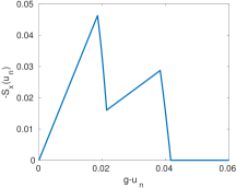
Figure 5: Regularized delamination law $S_{x}$ for $\varepsilon=10^{-4}$

The discrete Lagrange multiplier $\lambda^{\varepsilon}_{hp}$ is obtain by solving (48) where $\psi_{i}$ are discontinuous, piecewise polynomials on $\Gamma_{C}$ on a one time coarsened mesh $(H=2h)$ with polynomial degree reduced by one $(q=p-1)$ compared to the mesh and polynomial degree distribution of $\mathbf{u}^{\varepsilon}_{hp}$. Figure 6 displays the deformation of the rectangle and the normal stresses on $\Gamma_{C}$ obtained from the lowest order uniform $h$-method with 16384 elements and regularization parameter $\varepsilon=10^{-4}$. The normal stress on $\Gamma_{C}$, Figure 6 (b), reflects the delamination law from Figure 5 well.

  

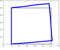
(a) Deformation

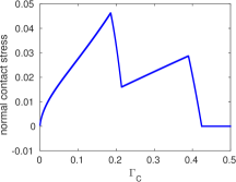
(b) Contact stresses

Figure 6: Uniform $h$-version, p=1, 16384 elements with 4096 elements on $\Gamma_{C}$

Figure 7 displays the reduction of the error in $(\mathbf{u},\lambda)$ and of the error estimate. Since the exact solution is not known, we compute the error approximately by $\|\mathbf{u}_{fine}-\mathbf{u}_{hp}\|_{P}$ and $\|\lambda_{fine}-\lambda_{hp}\|_{V}$, with norms induced by the Poincaré-Steklov operator, single layer potential acting on $\Gamma_{C}$, respectively. The pair $(\mathbf{u}_{fine},\lambda_{fine})$ is a very fine (last) approximation for each sequence of discretization. These error expressions are only meaningful if the distance is sufficiently large, which at the end of the different discretization sequences is not true and, therefore, are then omitted. Hence, the error curves are ”shorter” then the error estimate curves.
The uniform $h$-version with $p=1$ exhibits an experimental order of convergence (eoc) of 0.65 for the error and of 0.53 for the error estimate, all w.r.t. degrees of freedom (dof). Hence, the error estimate is only reliable but not efficient. For the $h$-adaptive scheme with $p=1$, the eoc is 0.84 for the error and only 0.56 for the error estimate over the last 20, 10 iterations, respectively. In case of $hp$-adaptivity the eoc appears to be exponential for the error and 1.52 for the error estimate also over the last 10 iterations.

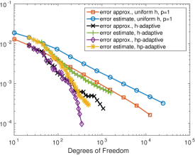
Figure 7: $\sqrt{\|\mathbf{u}_{fine}-\mathbf{u}_{hp}\|_{P}^{2}+\|\lambda_{fine}-\lambda_{hp}\|_{V}^{2}}$ and error estimate for different families of discrete solutions, $\varepsilon=10^{-4}$

Looking at the single contributions of the error estimate plotted in Figure 8 we find that in all cases the complementarity contribution is the dominant error contribution with the lowest order of convergence and that the consistency contribution has always a significantly higher order of convergence. Given the nature of this numerical experiment, the violation of the non-penetration condition is always zero and, therefore, is omitted in these plots. For the uniform $h$-version, Figure 8 (a), we have that the Neumann and $V^{-1}$ contributions converge at $0.62$ almost as fast as the error approximation. Given the nature, that $\lambda_{h,1}$ is piecewise constant with double mesh size, $-\mathbf{u}_{h,1}\cdot\mathbf{n}$ is linearly increasing and thus $-S_{x}(\mathbf{u}_{h,1}\cdot\mathbf{n})$ in the simplest case as well, the complementarity contribution is zero on the left element and non-zero on the right element. This oscillatory case occurs over a large fraction of $\Gamma_{C}$ and thus the $h$-adaptive scheme performs almost uniform mesh refinements on $\Gamma_{C}$, c.f. Figure 9(a). Hence, the little gain in $h$-adaptivity, Figure 8 (b), for the error estimate. This oscillatory effect can be reduced by increasing the polynomial degree as in $hp$-adaptivity, which balances out the single error contributions, Figure 8 (c) and is thus capable of producing more localized refinements, c.f. Figure 9(b).

 

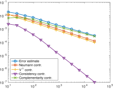
(a) uniform $h$-version with $p=1$

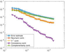
(b) $h$-adaptive with $p=1$

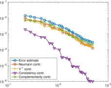
(c) $hp$-adaptive

Figure 8: Error contributions of the error estimates

  

\begin{overpic}[trim=81.09035pt 28.45274pt 64.01869pt 15.649pt,clip,clip,width=156.49014pt,keepaspectratio]{mesh_h_20.pdf} \put(6.5,8.0){\includegraphics[trim=83.93562pt 19.91692pt 65.44133pt 8.53581pt,clip,clip,width=133.72795pt,keepaspectratio]{mesh_h_10.pdf}} \end{overpic}

(a) $h$-adaptive, mesh nr. 10 (inner), nr. 20 (outer)

\begin{overpic}[trim=81.09035pt 28.45274pt 64.01869pt 15.649pt,clip,clip,width=156.49014pt,keepaspectratio]{mesh_hp_25.pdf} \put(6.7,8.0){\includegraphics[trim=78.24507pt 19.91692pt 61.17342pt 8.53581pt,clip,clip,width=133.72795pt,keepaspectratio]{mesh_hp_15.pdf}} \end{overpic}

(b) $hp$-adaptive, mesh nr. 15 (inner), nr. 25 (outer)

Figure 9: Adaptively generated meshes

Finally, Figure 10 shows the influence of the regularization parameter on the errors $\|\mathbf{u}_{fine}-\mathbf{u}_{h,1}^{\varepsilon}\|_{P}$ and $\|\lambda_{fine}-\lambda_{h,1}^{\varepsilon}\|_{V}$ where $(\mathbf{u}_{fine},\lambda_{fine})$ is the Galerkin solution to a uniform mesh with 16384 elements, $p=1$ and regularization parameter $\varepsilon=2.5\cdot 10^{-6}$. Here, the pair $(\mathbf{u}_{h,1}^{\varepsilon},\lambda_{h,1}^{\varepsilon})$ is computed on a uniform mesh with 8192 elements and the regularization parameter is varied. We find that for very large $\varepsilon$, the regularized delamination law has lost its saw tooth characteristic and small variations of $\varepsilon$ have no noticeable influence. For very small $\varepsilon$ the discretization error is dominant which sets in for $\mathbf{u}$ much earlier than for $\lambda$. In the intermediate range the eoc w.r.t. $\varepsilon$ is 0.75 for $\mathbf{u}$, whereas $\lambda$ displays an (asymptotic) eoc of 1.0 w.r.t. $\varepsilon$. The error estimate for the regularized problem increases in $\varepsilon$ slightly.

Acknowledgment The authors are grateful to J. Gwinner for the helpful discussions and comments.

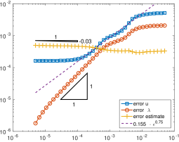
Figure 10: Error and error estimate for different regularization parameters $\varepsilon$, uniform $h$-version 8192 elements, $p=1$

References

- (1) Attouch, H.: Variational convergence for functions and operators. Pitman, Boston (1984)
- (2) Banz, L., Gimperlein, H., Issaoui, A., Stephan, E.P.: Stabilized mixed -BEM for frictional contact problems in linear elasticity. Numer. Math. (2016). DOI: 10.1007/s00211-016-0797-y
- (3) Banz, L., Stephan, E.P.: A posteriori error estimates of -adaptive IPDG-FEM for elliptic obstacle problems. Appl. Numer. Math. 76, 76–92 (2014)
- (4) Banz, L., Stephan, E.P.: On hp-adaptive BEM for frictional contact problems in linear elasticity. Comput. Math. Appl. 69(7), 559–581 (2015)
- (5) Bernardi, C., Maday, Y.: Spectral methods. In: Handb. Numer. Anal., vol. V, pp. 209–485. North-Holland, Amsterdam (1997)
- (6) Braess, D.: A posteriori error estimators for obstacle problems–another look. Numer. Math. 101(3), 415–421 (2005)
- (7) Carstensen, C.: Interface problem in holonomic elastoplasticity. Math. Methods Appl. Sci. 16(11), 819–835 (1993)
- (8) Carstensen, C.: A posteriori error estimate for the symmetric coupling of finite elements and boundary elements. Computing 57(4), 301–322 (1996)
- (9) Carstensen, C., Funken, S.A., Stephan, E.P.: On the adaptive coupling of FEM and BEM in 2–d–elasticity. Numer. Math. 77(2), 187–221 (1997)
- (10) Carstensen, C., Gwinner, J.: FEM and BEM coupling for a nonlinear transmission problem with Signorini contact. SIAM J. Numer. Anal. 34(5), 1845–1864 (1997)
- (11) Chernov, A.: Nonconforming boundary elements and finite elements for interface and contact problems with friction - hp-version for mortar, penalty and Nitsche’s methods. Ph.D. thesis, Universität Hannover (2006)
- (12) Chernov, A., Maischak, M., Stephan, E.P.: hp-Mortar boundary element method for two-body contact problems with friction. Math. Methods Appl. Sci. 31(17), 2029–2054 (2008)
- (13) Clarke, F.H.: Optimization and nonsmooth analysis. John Wiley and Sons (1983)
- (14) Costabel, M.: Boundary integral operators on Lipschitz domains: Elementary results. SIAM J. Math. Anal. 19(3), 613–626 (1988)
- (15) Costabel, M., Stephan, E.P.: Coupling of finite and boundary element methods for an elastoplastic interface problem. SIAM J. Numer. Anal. 27(5), 1212–1226 (1990)
- (16) Dao, M., Gwinner, J., Noll, D., Ovcharova, N.: Nonconvex bundle method with application to a delamination problem. Computational Optimization and Applications (2016). DOI: 10.1007/s10589-016-9834-0
- (17) Glowinski, R.: Numerical methods for nonlinear variational problems. Springer Series in Computational Physics (1984)
- (18) Guediri, H.: On a boundary variational inequality of the second kind modelling a friction problem. Math. Methods Appl. Sci. 25(2), 93–114 (2002)
- (19) Gwinner, J.: Nichtlineare Variationsungleichungen mit Anwendungen. Ph.D. thesis, Universität Mannheim (1978)
- (20) Gwinner, J.: hp-FEM convergence for unilateral contact problems with Tresca friction in plane linear elastostatics. J. Comput. Appl. Math. 254, 175–184 (2013)
- (21) Gwinner, J., Ovcharova, N.: From solvability and approximation of variational inequalities to solution of nondifferentiable optimization problems in contact mechanics. Optimization (ahead-of-print), 1–20 (2015)
- (22) Gwinner, J., Stephan, E.P.: A boundary element procedure for contact problems in linear elastostatics. ESAIM Math. Model. Numer. Anal. 27(4), 457 – 480 (1993)
- (23) Han, H.D.: A direct boundary element method for Signorini problems. Math. Comp. 55(191), 115–128 (1990)
- (24) Houston, P., Süli, E.: A note on the design of hp-adaptive finite element methods for elliptic partial differential equations. Comput. Methods Appl. Mech. Engrg. 194(2-5), 229–243 (2005)
- (25) Hsiao, G.C., Wendland, W.L.: Boundary integral equations. Springer (2008)
- (26) Kleiber, M., Borkowski, A.: Handbook of computational solid mechanics: survey and comparison of contemporary methods. Springer (1998)
- (27) Krebs, A., Stephan, E.: A p-version finite element method for nonlinear elliptic variational inequalities in 2D. Numer. Math. 105(3), 457–480 (2007)
- (28) Maischak, M., Stephan, E.P.: A FEM–BEM coupling method for a nonlinear transmission problem modelling Coulomb friction contact. Comput. Methods Appl. Mech. Engrg. 194(2), 453–466 (2005)
- (29) Maischak, M., Stephan, E.P.: Adaptive hp-versions of BEM for Signorini problems. Appl. Numer. Math. 54(3), 425–449 (2005)
- (30) Maischak, M., Stephan, E.P.: Adaptive hp-versions of boundary element methods for elastic contact problems. Comput. Mech. 39(5), 597–607 (2007)
- (31) Nesemann, L., Stephan, E.P.: Numerical solution of an adhesion problem with FEM and BEM. Appl. Numer. Math. 62(5), 606–619 (2012)
- (32) Ovcharova, N.: Regularization Methods and Finite Element Approximation of Hemivariational Inequalities with Applications to Nonmonotone Contact Problems. Ph.D. thesis, Universität der Bundeswehr München (2012)
- (33) Ovcharova, N.: On the coupling of regularization techniques and the boundary element method for a hemivariational inequality modelling a delamination problem. Math. Methods Appl. Sci. (2015). ArXiv 1603.05091
- (34) Ovcharova, N., Gwinner, J.: A study of regularization techniques of nondifferentiable optimization in view of application to hemivariational inequalities. J. Optim. Theory Appl. 162(3), 754–778 (2014)
- (35) Sloan, I.H., Spence, A.: The Galerkin method for integral equations of the first kind with logarithmic kernel: Theory. IMA J. Numer. Anal. 8(1), 105–122 (1988)
- (36) Steinbach, O.: Numerische Näherungsverfahren für elliptische Randwertprobleme: Finite Elemente und Randelemente. Vieweg + Teubner (2003)
- (37) Stephan, E.P.: The hp-version of BEM—fast convergence, adaptivity and efficient preconditioning. J. Comput. Math. 27(2-3), 348–359 (2009)
- (38) Wetzel, M., Holtmannspötter, J., Gudladt, H.J., Czarnecki, J.: Sensitivity of double cantilever beam test to surface contamination and surface pretreatment. Int. J. Adhes. Adhes. 46, 114–121 (2013)