Fitting High-Dimensional Interaction Models with Error Control

Abstract

There is a renewed interest in polynomial regression in the form of identifying influential interactions between features. In many settings, this takes place in a high-dimensional model, making the number of interactions unwieldy or computationally infeasible. Furthermore, it is difficult to analyze such spaces directly as they are often highly correlated. Standard feature selection issues remain such as how to determine a final model which generalizes well. This paper solves these problems with a sequential algorithm called Revisiting Alpha-Investing (RAI). RAI is motivated by the principle of marginality and searches the feature-space of higher-order interactions by greedily building upon lower-order terms. RAI controls a notion of false rejections and comes with a performance guarantee relative to the best-subset model. This ensures that signal is identified while providing a valid stopping criterion to prevent over-selection. We apply RAI in a novel setting over a family of regressions in order to select gene-specific interaction models for differential expression profiling.

, , and

backgroundcolor=blue!20!white,inline, bordercolor=red]Bob: Bottom line: Impressive results. Repackage as “Fitting high dimensional interaction models” (or something like that), lead with the strong simulated examples (and hopefully a real one chosen from biology), then add theory as needed to justify what you are doing.

backgroundcolor=blue!20!white,inline, bordercolor=red]Go through entire document and make claims asymptotic. Check for all use of gaussian or normal etc

1 Introduction

We study the problem of selecting predictive features from a large feature space. Our data consists of $n$ i.i.d. observations of (response, feature) sets, where each observation has $m$ associated features: $(y_{i},x_{i1},\ldots,x_{im})\sim\mathcal{P}$. As we are interested in models using not only these $m$ raw features (main effects) but also polynomials of the features (interaction effects), we consider an expanded feature space of dimension $d$ which is created by extending our data set as ($y_{i},x_{i1},\ldots,x_{im},x_{i(m+1)},\ldots,x_{id})$. Each $x_{ik}$ for $k\in\{m+1,\ldots,d\}$ is a product of raw features: rCl x_ik & = ∏_j=1^m x_ij^ξ_kj, where $\xi_{kj}$ is the power of feature $j$ in the interaction $k$. In general, we do not place a constraint on either the value of $\xi_{kj}$ or the number of features $j$ that are allowed in the interaction, as these characteristics will be adaptively determined by our procedure. The complete feature space, however, is best thought of as all interactions which can be created with the restriction that $\sum_{j=1}^{m}\xi_{kj}\leq\kappa$, for some $\kappa\in\mathbb{N}$.

Observations are collected into matrices and the following model is assumed for our data rCl+rCl Y & = μ(X)+ ϵ ϵ ∼ N_n(0,σ^2 I_n) where $\mathbf{X}\in\mathbb{R}^{n\times m}$ and $Y\in\mathbb{R}^{n}$. We will produce linear estimates of the true conditional mean $\mu(\mathbf{X})$ of the form $\hat{Y}=\mathbf{X}\hat{\beta}$ for $\hat{\beta}\in\mathbb{R}^{d}$. As we fit linear models which always include an intercept, we assume without loss of generality that our raw features are mean zero, $\sum_{i}y_{i}=\sum_{i}x_{ij}=0$, $\forall j\leq m$, and normalized such that $\text{Var}(Y)=\text{Var}(X_{j})=1$, $\forall j\leq m$. While we fit linear models and conduct hypothesis tests on estimated coefficients, we do not assume that we are testing within the true linear model or that one even exists. Instead, we view null hypotheses in terms of projections of the true mean on the observed data as in Abadie14, also known as the “$\mathbf{X}$-conditional parameter” in Buja+18. This is necessary as we will be performing hypothesis tests multiple times in many different models. More details are given in Section 2.

Generating good predictions requires identifying a comparatively small subset of predictive features. In modern applications, $d$ is often exceedingly large, which makes the selection of an appropriate subset of these features essential. The model selection problem is to minimize the error sum of squares rCl ESS(^Y) = ∥Y - ^Y∥^2_2 = ∑_i=1^n (Y_i - ^Y_i)^2 while restricting the number of nonzero coefficients: c’t’rCl min_δ∈R^d ESS(Xδ) & s.t. ∥δ∥_l_0 = ∑_i=1^d I_{δ_i≠0} ≤K, where the number of nonzero coefficients, $K$, is the desired sparsity. Note that we are not assuming that a sparse true model exists, merely asking for a sparse approximation. In the statistics literature, the model selection problem (1) is more commonly posed as a penalized regression: rCl ^β_0,λ & = argmin_δ{ESS(Xδ) + λ∥δ∥_l_0 } where $\lambda\geq 0$ is a constant. The classical hard thresholding algorithms $C_{p}$ (Mal73), AIC (Aka74), BIC (Schwarz78), and RIC (FosterG94) vary $\lambda$. The solution to (1) is the least-squares estimator on an optimal subset of features. Let $M\subset\{1,\ldots,d\}$ indicate the coordinates of a given model so that $\mathbf{X}_{M}$ is the corresponding submatrix of the data. If $M_{\lambda}^{*}$ is the optimal set of features for a given $\lambda$, then $\hat{\beta}_{0,\lambda}^{*}=\mathbf{X}_{M_{\lambda}^{*}}^{\dagger}Y$, where $\mathbf{X}_{M_{\lambda}^{*}}^{\dagger}$ is the pseudoinverse of $\mathbf{X}_{M_{\lambda}^{*}}$.

Given the combinatorial nature of the constraint, solving (1) quickly becomes infeasible as $d$ increases and is NP-hard in general (Nata95). Forward stepwise is the greedy approximation to the solution of (1). Let $M_{i}$ be the features in the forward stepwise model after step $i$ and note that the size of the model is $|M_{i}|=i$. The algorithm is initialized with $M_{0}=\emptyset$ and iteratively adds the variable which yields the largest reduction in ESS. Hence, $M_{i+1}=\{M_{i}\cup j\}$ where

$$j=\operatorname*{arg\,max}_{l\in\{1,\ldots,d\}\backslash M_{i}}\text{ESS}(\mathbf{X}_{M_{i}\cup l}\hat{\beta}_{M_{i}\cup l}^{\text{LS}}).$$

After the first feature is selected, subsequent models are built having fixed that feature in the model. $M_{1}$ is the optimal size-1 model, but $M_{i}$ for $i\geq 2$ is not guaranteed to be optimal, because $M_{i}$ is forced to include the features identified at previous steps.

To illustrate our method, consider the concrete compressive strength data from the UCI machine learning repository (concrete-data). It is important to note that our goal is to identify interactions in contexts in which interpreting such features is desirable. Precise examples of this sort are provided in Section 5. For now, our goal is to demonstrate the ability to search such a space to find signal over competing methods. This data set is used because the response, compressive strength, is described as a “highly nonlinear function of age and ingredients” such as cement, fly ash, water, superplasticizer, etc. It is also useful since it has approximately 1000 observations and only 8 features. A small number of features is needed so that a large, higher-order interaction space can be generated in order to see how standard feature selection algorithms perform. All interactions up to fourth order are provided to competitor algorithms, in which case there are 1,124 features.

This paper presents an algorithm, Revisiting-Alpha Investing (RAI), that is able to adaptively search a high-dimensional interaction space by building interactions from previously selected components. This is done while controlling a notion of false rejections. While the details are presented in Section 4, the idea of RAI is easy to describe: RAI is provided the raw features, and conducts an approximate version of stepwise regression on these features. Instead of selecting the feature which is most significant, it merely includes features which are significant enough to pass an appropriate statistical test. When a feature is included in the model, all possible interactions with previously selected features are added to the searchable feature space. Stepwise selection then continues on this expanded feature space. Furthermore, it is often useful to search for interactions of transformed features, e.g. after taking the square-root. This allows a fourth-degree polynomial among the new features to be merely a second-degree polynomial among the original features. We compare RAI to forward stepwise, backward stepwise, Lasso, and FOBA (Zhang08). FOBA stands for “forward-backward” and is an algorithm with both sequentially adds and deletes features. In this data example, we also use our implementation of stepwise as other implementations were not able to cope with even problems of this size.

To estimate out-of-sample performance, we create 10 independent splits of the data into training and test sets, where 25% of the data is used for testing. We select the parameters of the models using using 5-fold cross-validation using the training data and measure performance of the CV-selected model on the test set. We compare models using the predictive root-mean-squared error (RMSE) on the test set and average model size. Each row in Table 1 indicates the explanatory features that the algorithms are provided. For example, the first row shows the performance results when all algorithms are only given raw features to estimate main effects, while in subsequent rows the competitor algorithms are given all second order interactions etc. We only consider models up to fourth-order interactions due to the computational limitations of competitor algorithms. This also motivates the desire for a stepwise solution, as other standard algorithms are unable to select satisfactory models from interaction spaces.

backgroundcolor=blue!20!white,inline, bordercolor=red]plot of MSE on size: get same MSE need more features

Table 1: Concrete Compression Strength Results.

Set	Statistic	foba	lasso	lm	rai	raiStep
$\mathbf{X}$	RMSE	10.05	10.05	10.08	7.70	10.09
$p=11$	Model Size	7.30	9.40	11.00	18.60	5.90
$\mathbf{X}^{2}$	RMSE	7.66	7.57	7.47		8.00
$p=74$	Model Size	40.80	66.10	74.00		12.30
$\mathbf{X}^{3}$	RMSE	6.54	8.09e9	16.81		7.59
$p=326$	Model Size	59.80	288.20	326.00		16.20
$\mathbf{X}^{4}$	RMSE	19.19	7.55e20	1.73e6		7.50
$p=1124$	Model Size	86.30	562.30	1124.00		20.30

There are several important points in Table 1. As expected, RAI is superior to other feature selection methods when only considering marginal features, as the other algorithms do not extend the feature space to consider interactions; however, we can adjust for the information differences by giving the competitor algorithms a richer feature space. When given second order interactions, the other algorithms have effectively the same performance as RAI but select far more features. Furthermore, as the feature space gets more complex, the inherent difficulty becomes apparent as the RMSE of the lasso and the full linear model explode. FOBA actually continues to improve for third order interactions before worsening, though it still selects many more features. Unfortunately, the computational complexity of FOBA is even worse than classical stepwise, so we are unable to use it in larger examples considered later. Lastly, it is worth noting that our implementation of forward stepwise has a stopping criterion that prevents it from over-selecting: the performance does not change drastically as we go beyond second order interactions. Furthermore, the final model selected using RAI on raw features behaves very similarly to the stepwise model selected from all forth order interactions. As such, RAI is adequately searching this space in a stepwise fashion.

The remainder of the paper is organized as follows. Section 2 provides the notation and definitions necessary to state our main results. Section 3 introduces our threshold approximations via the conceptually simpler Revisiting Holm procedure. This section begins with a motivating example to demonstrate the differences between post-selection inference and using inference to perform model selection. Section 4 provides a more complex threshold procedure which overcomes the shortcoming of Revisiting Holm and has performance guarantees. The benefits and validity of these procedures are demonstrated via simulation in Section 4.4. The interaction-search procedure described above is explained in Section 5, which includes a novel methodology differential expression profiling. Section LABEL:sec:discussion concludes.

2 Notation and Results

We use notation from the multiple comparisons literature given its connection to our solution. Consider $l$ null hypotheses, $H_{[l]}$: $H_{1},\ldots,H_{l}$, and their associated p-values, $p_{[l]}$: $p_{1},\ldots,p_{l}$. The notation $[l]=\{1,\ldots,l\}$ will be used frequently for any $l\in\mathbb{N}$. The hypotheses are sequential, meaning they arrive in a sequence and one must decide whether or not to reject test $H_{i}$ before knowing any information about $H_{i+1}$. In general, the order of hypotheses can depend on the sequence of rejections, but this is not the focus of the current discussion so is ignored. As sorting p-values is frequently required, we use standard order statistic notation: $p_{(1)}\leq p_{(2)}\leq\ldots\leq p_{(l)}$. Note that this same ordering extends to both hypotheses and features: $H_{(k)}$ and $X_{(k)}$ are the hypothesis and feature corresponding to $p_{(k)}$, respectively.

As we analyze forward stepwise, each null hypothesis assumes that the fit of $M$ is not improved by adding a feature $\mathbf{X}_{j}$: rCl H_i^M,j: P_Mμ(X) & = P_M ∪jμ(X), where $M$ is a set of indices specifying the columns of $\mathbf{X}$ in the current model, $P_{M^{\prime}}=\mathbf{X}_{M^{\prime}}\mathbf{X}_{M^{\prime}}^{\dagger}$ is the projection matrix onto the column-span of $\mathbf{X}_{M^{\prime}}$, and $\mathbf{X}_{M^{\prime}}^{\dagger}$ is the pseudo-inverse of $\mathbf{X}_{M^{\prime}}$ for any $M^{\prime}\subset[m]$. Similarly, $P_{M^{\prime\perp}}=\mathbf{I}-P_{M^{\prime}}$ is the projection onto the space orthogonal to the column-space of $\mathbf{X}_{M^{\prime}}$. In equation (2), the null hypothesis depends on the data $\mathbf{X}$.

The sub- and super-scripts in equation (2) are unrelated. The subscript $i$ merely counts the index of the test whereas the superscripts $M$ and $j$ determine the test. Sometimes scripts will be dropped when only the index of the test, $i$, or the identity of the test, $\{M,j\}$, is required (these conventions also apply to $R$ and $V$ defined below). Note that order statistic notation extends here as well. Given a set of hypotheses $H^{M,1},\ldots,H^{M,l}$, their corresponding sorted p-values are $p^{M,(1)}\leq p^{M,(2)}\leq\ldots\leq p^{M,(l)}$. The comparisons here are legitimate because all $l$ tests are conducted within the same base model $M$.

Note that our null hypothesis is equivalent to testing the coefficient on $\mathbf{X}_{j}$ in the model $M^{\prime}=M\cup j$. Additional care must be taken with these tests as we are not assuming to be testing in the correct model. Abadie14 provide a standard error estimate that is robust to model mis-specification for our $\mathbf{X}$-conditional parameter. In practice, we use a more conservative estimator for computational efficiency as explained in Section 4. Given such an estimate, $\hat{\sigma}$, the classical test statistic in this setting is

$$z^{[M,j]}=\frac{Y^{\prime}P_{M^{\perp}}\mathbf{X}_{j}}{\hat{\sigma}\sqrt{\mathbf{X}_{j}P_{M^{\perp}}\mathbf{X}_{j}}}.$$

As we are using classical p-values, one may wonder at the connections to classical rules to stop forward stepwise such as F-to-enter or F-to-delete. It was previously demonstrated that such tests do not control any robust statistical quantity, because attempting to test the addition of new features uses non-standard and complex distributions (DraperGK71; PopeW72). This critiques are not relevant to our setting, because we are using this aforementioned, model-dependent target and modifying the stepwise routine to account for selection.

Define the statistic $R_{i}^{M,j}=1$ if $H_{i}^{M,j}$ is rejected and $R_{i}^{M,j}=0$ if not. Similarly, let $V_{i,\mu}^{M,j}=1$ if $R_{i}^{M,j}=1$ is a false rejection ($H_{i}^{M,j}$ is true) and $V_{i,\mu}^{M,j}=0$ if not. The dependence of $V_{i,\mu}^{M,j}$ on $\mu$ indicates that it is an unobserved random variable which depends on the unknown mean. For simplicity, all future uses of $V_{i,\mu}^{M,j}$ suppresses this notation. Define rCl’t’rCl R(l) & = ∑_i=1^l R_i and V(l) = ∑_i=1^l V_i, to be the total number of rejections and false rejections in the $l$ sequential tests, respectively.

Our method controls the marginal false discovery rate (mFDR) which is similar to the more common false discovery rate (FDR):

Definition 1 (Measures of the Proportion of False Discoveries).

rCl mFDR(l) & = E(V(l))E(R(l))+1
FDR(l) = E(V(l)R(l)), where 00 = 0.

In some respects, FDR is preferable to mFDR because it controls a property of a realized distribution. While not observed, the ratio $V(l)/R(l)$ is the realized proportion of false rejections. FDR controls the expectation of this quantity. In contrast, mFDR is not a property of the distribution of $V(l)/R(l)$. That being said, FDR and mFDR behave nearly identically in practice, and mFDR yields a powerful and flexible martingale (FosterS08). This martingale provides the basis for proofs of mFDR control in a variety of situations.

Our first contribution is an elucidation of the effects that must be considered when using hypothesis testing for model selection. Standard inference tools are invalid due to two selection effects: the ranking effect and the testing effect. The ranking effect is the result of testing hypotheses that are suggested by the data and the testing effect is the result of only conducting future tests if previous tests have been rejected. The impacts of these effects are explained via example in Section 3.1.

In Sections 3 and 4, we demonstrate that the sequential testing approach to multiple comparisons yields an approximate forward stepwise algorithm that controls for the selection effects. We provide three procedures of increasing complexity: Revisiting-Holm (RH), Revisiting-Alpha-Investing (RAI), and RAI⁺. RH is introduced in Section 3 purely as a conceptual tool to aid understanding. RAI is provided in Section 4 to avoid serious pitfalls of RH, and RAI⁺ provides minor adjustments to the procedure to enjoy stronger theoretical guarantees. In practice, RAI and RAI⁺ behave essentially identically.

All of the procedures are threshold approximations to stepwise regression. At each step, forward stepwise computes and sorts the sequential p-values for adding each of the remaining $m^{\prime}$ features to the current model $M$, $p^{M,(1)}\leq\ldots\leq p^{M,(m^{\prime})}$, and selects the feature with the minimum p-value. Instead of performing a full sort, threshold approximations use a set of increasing rejection thresholds, and hypotheses are rejected when their p-value falls below a threshold. A feature merely needs to be significant enough, not necessarily the most significant. The initial rejection threshold conducts a strict test for which only highly significant features are added to the model. Subsequent thresholds perform less stringent tests. As such, the final model is built from a series of approximately greedy choices.

While stepwise-regression is a traditionally slow procedure, RAI and RAI⁺ achieve a dramatic increase in speed by conducting individual, sequential tests and taking advantage of Variance Inflation Factor Regression (LinFU11). If the final model size is of smaller order than $\min(n,m)$, the computational complexity of RAI grows at $O(nm\log(n))$. Using the full data requires computing $\mathbf{X}^{\prime}y$, which takes $O(nm)$ time. Therefore, RAI merely adds a log factor to perform valid model selection.

Our first result shows that sequential, classical tests are conditionally of level $\alpha$ when the null hypotheses are augmented for previously failed tests. For example, if we fail to reject $H_{i}^{M,j}:P_{M}\mu(\mathbf{X})=P_{M\cup j}\mu(\mathbf{X})$, then the next test is under the null-hypothesis, $H_{i+1}^{M,j^{\prime}}:P_{M}\mu(\mathbf{X})=P_{M\cup j}\mu(\mathbf{X})=P_{M\cup j^{\prime}}\mu(\mathbf{X})$. The alternative in this case is still the same, ie, that $P_{M}\mu(\mathbf{X})\neq P_{M\cup j^{\prime}}\mu(\mathbf{X})$. This does not yield the most powerful test of this null hypothesis, but it is consistent with our use of a rejection of it. While such augmentation may not generally be palatable, it is natural in the sequential setting, only concerns the set of failed hypothesis tests, and allows us to leverage the Gaussian Correlation Inequality (Royen14; LatM15) in the proof of the following theorem.

Theorem 1.

Using an estimate of $\hat{\sigma}$ which is robust to model misspecification, the sequential testing methods RAI and RAI⁺ ensure

$$\mathbb{E}(V_{i}|R_{1},\ldots,R_{i-1})\leq\alpha_{i}$$

for every $i<n$ under the augmented null-hypothesis.

Note that this holds regardless of the correlation structure between the columns of $\mathbf{X}$ due to normality. The constraint on the maximum number of tests $i$ is due to augmenting the null hypothesis for all failed tests. More information on this construction and its implications are in Appendix LABEL:app:valid-tests. With Theorem 1 in hand, all of our procedures control mFDR as they are alpha-investing rules (FosterS08). The algorithms are presented independently of alpha-investing so that the algorithm and proof method are not conflated.

Corollary 1.

RAI and RAI⁺ control mFDR: rCl E(V(m))E(R(m))+1 ≤α.

Theorem 1 and Corollary 1 are in some ways similar to other post-selection inference methods but the perspective is very different. Berk+13 adjust for the potentially adversarial instance in which a final model is selected to influence the test-statistic of one of the features. Selective inference (FithST15; Taylor+14) control the selective type-I error, which conditions on the event that the model $M$ and null hypothesis $H_{0}$ were selected for testing.

We do not control this selective error rate, because the hypothesis we are testing is not actually intentionally selected, so to speak, based on some criteria. We do not test a feature in a given model because it has the minimum p-value, for example. Instead, we produce an algorithm which agnostically generates a set of rejections with the desired properties while paying sufficient alpha-wealth for their discovery. In this way, we need not condition on the question being asked as in selective inference, but on the set of answers, ie rejections, that led us to the current test. This subtle distinction allows us to leverage classical hypothesis tests. In an important sense, we are not doing the “data snooping” that invalidates these tests.

A second type of result concerns the approximation guarantee between RAI⁺ and stepwise regression. While we are not guaranteed to select the same model as forward stepwise, we are able to guarantee that the in-sample fit we achieve is comparable to that of forward stepwise and the ideal model. Our measure of model fit for a set of features $\mathbf{X}_{M}$ is the coefficient of determination, R², defined as

$$\text{R${}^{2}$}(M)=1-\frac{ESS(\mathbf{X}_{M}\hat{\beta}_{M})}{ESS(\bar{Y})}$$

where $\bar{Y}$ is the constant vector of the mean response and $\hat{\beta}_{M}$ is the least squares estimate for predicting $Y$ from $\mathbf{X}_{M}$. Corollary 1 coupled with Theorem 2 below demonstrate that RAI⁺ identifies signal (measured in-sample), but controls for over-fitting by not making too many incorrect selections.

In the following theorem, for $r\in(0,1)$, $r^{s}$ is the threshold for improvement in R² used on the $s$th testing pass. For example, if $r=1/2$, then the first testing pass searches for features which increase R² by 1/2, while the second searches for those yielding an increase of 1/4. This yields a geometrically decreasing sequence of bounds. The translation between these R² thresholds to p-value thresholds is given in the proof of the theorem. The theorem compares the performance of the selected set of $l$ features, $M_{l}$, and the best performing set of $k$ features, $M_{k}^{*}$. The term $\gamma$ is similar in spirit to the restricted-eigenvalue condition (RasWY10), but is less restrictive and tailored to our setting. It is also lower bounded by a sparse eigenvalue. A full discussion is provided in Section 4. As will be seen in the proof, most instances of the procedure use a bound that is much better than $\gamma$, as control with respect to models of this size is only required in cases when all features in the final model are rejected in a single pass. This only occurs in specially created scenarios.

Theorem 2.

RAI⁺ selects a set of features $M_{l}$ of size $l$ such that rCl R²(M_l) & ≥ (1-e^l/c)R²(M_k^*) where $c=\left(\frac{\iota+k}{\gamma r}-\iota\right)$ and $\iota$ is the maximum number of features rejected in a testing pass.

As $r\to 1$, $\iota\to 0$, and RAI⁺ converges to stepwise regression. In this case, Theorem 2 recovers the usual bound for stepwise regression $\text{R${}^{2}$}(S_{l})\geq(1-e^{l\gamma/k})\text{R${}^{2}$}(S_{k}^{*})$, which is also proven in the appendix.

If the approximation guarantee given above is insufficient and using the exact forward stepwise path is desired, GSell+15 provide a method for turning a sequence of valid, independent, post-selection p-values into a model selection procedure. While these p-values cannot be validly used to select a model (BrownJ16comm), they derive a procedure in this case called ForwardStop, which can be seen as a limiting case of RAI. This produces a final procedure, Stepwise-RAI (S-RAI), for use in small models and also demonstrates why ForwardStop has low power. Furthermore, S-RAI is able to perform valid model selection using traditional, stepwise p-values.

The sequential testing framework of RAI allows the order of tested hypotheses to be changed as the result of previous tests. This allows for directed searches in data base queries or identifying interactions. Section 5 leverages this flexibility to greedily search high-order interactions spaces. Such directed search does not invalidate Theorem 1 or Corollary 1 as future tests or orthogonal to previous rejections; however, the performance guarantee needs to be modified and is presented in in Section 5. We provide simulations and real data examples to demonstrate the success of our method.

3 Approximating Stepwise Regression

To motivate the construction of our revisiting procedure, it is instructive to consider the problem of stopping stepwise regression in a simple data setting. Consider the prostate cancer data used to motivate the inference methods of Taylor+14. The data set has 67 observations of 8 explanatory variables which will be used to predict the log PSA level of men who had surgery for prostate cancer. The traditional use of stepwise regression is summarized in Table 2. Each step of the procedure adds a feature to the model and assigns a p-value measuring the reduction in ESS using an F-test with independent $\hat{\sigma}$. The classical p-value does not take into account the fact that the hypothesis being tested is suggested by the data and algorithm. The second column of p-values in Table 2 are from Taylor+14 and adjust for selecting features using forward stepwise.

Table 2: Stepwise Regression: Prostate Cancer Data

Step	Parameter	Stepwise p-value	Adjusted p-value
1	lcavol	0.0000	0.000
2	lweight	0.0003	0.006
3	svi	0.0424	0.425
4	lbph	0.0468	0.168
5	ppg45	0.2304	0.423
6	lcp	0.0878	0.273
7	age	0.1459	0.059
8	gleason	0.8839	0.156

Our goal is to use the stepwise p-values in Table 2 to determine when to stop forward stepwise. For example, if it is claimed that the first 4 steps are significant but the 5th is not, the selected model will include lcavol, lweight, svi, and lbph. Such claims should be made solely on the basis of the p-values. We present a framework in which the traditional, stepwise p-values can be used to select a model. The p-values can provide preferable rejection regions to the adjusted tests of Taylor+14 (BrownJ16comm). We return to the adjusted p-values in Section 4.3 when comparing their use to one of our procedures. The difficulties in post-selection inference are accounted for within the testing framework instead of the p-value computation. This requires modifying the forward stepwise procedure but Theorem 2 guarantees we select a model which performs similarly.

3.1 Inference for Model Selection

Attempting to use inference for model selection poses significantly different challenges than merely performing inference after a model is selected. Inference will be conducted multiple times based on the result of previous inferential claims. A simple, orthogonal example distinguishes the different challenges posed by conducting inference multiple times. This separates questions about the statistical validity of repeated testing during forward stepwise from its ability to approximate the sparse regression problem (1): the model identified at the $k$th step of forward stepwise exactly solves (1) under orthogonality. That being said, constructing valid tests is still non-trivial due to the selection inherent in forward stepwise and repeated testing.

Suppose the data contain 10 orthogonal, explanatory features with true parameters $\beta_{1}=\ldots=\beta_{10}=0$ and $\sigma^{2}$ is known. In this case, the test statistics are iid $N(0,1)$ variables and are written with $z$. Furthermore, in the orthogonal setting test statistics and p-values do not change depending on the model in which they are estimated. Therefore, all statistics are assumed to be computed in simple regressions: $M=\emptyset$. The z-statistics for $H^{\emptyset,1},\ldots,H^{\emptyset,10}$ are $z^{\emptyset,1},\ldots,z^{\emptyset,10}$ with corresponding p-values $p^{\emptyset,1},\ldots,p^{\emptyset,10}$. The feature selection problem is equivalent to determining an order for testing $H^{\emptyset,[10]}$ while controlling a measure of false rejections at level $\alpha$. Since our goal is model selection, a feature is “included” or “added” to the model when the corresponding null hypothesis is rejected. Sort the hypotheses by their p-values $p^{\emptyset,(1)}<\ldots<p^{\emptyset,(10)}$. At step $i$, forward stepwise tests $H_{i}=H^{\emptyset,(i)}$ using test statistic $z_{i}$.

As expected, the distributions of the absolute order statistics are significantly different than the naive $|N(0,1)|$. Figure 1(a) and 1(b) show the distributions of $|z_{1}|$ and $|z_{3}|$, the magnitude of statistics chosen in steps 1 and 3. Informally, the difference between these distributions and the distribution of $|N(0,1)|$ is the ranking effect. This name is motivated as the difference between the test of a rank statistic and a randomly chosen one. Since our goal is not to estimate the correct distribution but to perform a valid, two-sided test, we desire a critical value yielding a level-$\alpha$ test. The nominal $\alpha=.1$ critical value is 1.645, whereas the simulated threshold is 2.58. This value can be easily computed using the Bonferroni correction, and the asymptotic, expected size of further rank statistics can be computed in the orthogonal case (GeorgeF00).

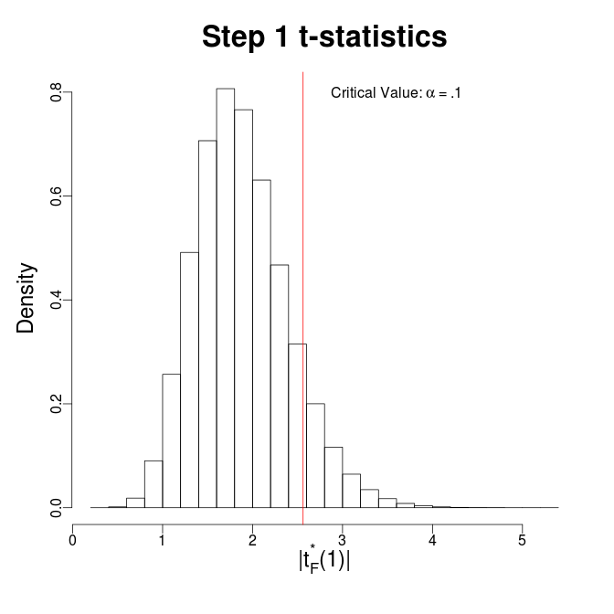
(a)

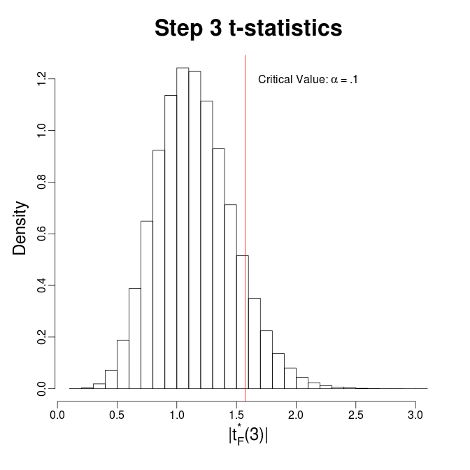
(b)

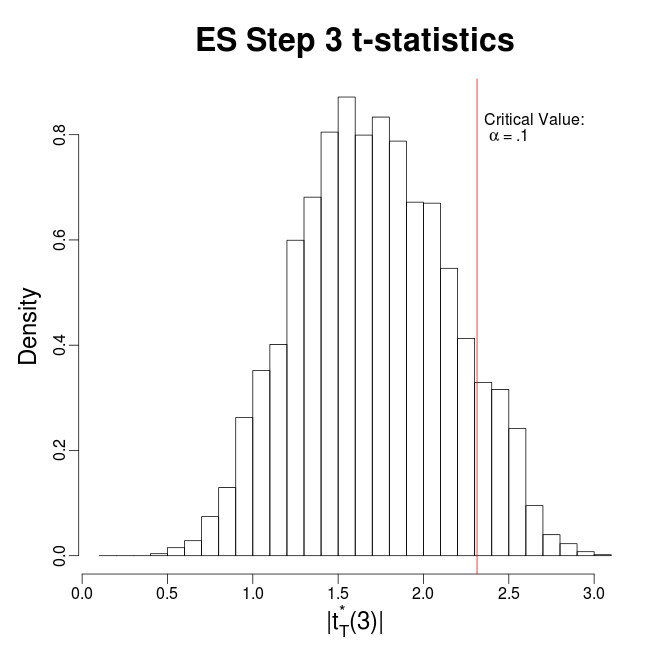
(c)

Figure 1: Illustration of selection and sequential effects under the global null hypothesis.

Consider a procedure in which forward stepwise is terminated on the first step in which a hypothesis fails to be rejected. In this case, $H_{i}$ is only tested if $H_{[i-1]}$ are all rejected. This procedure is discussed in BrownJ16comm. The simulated, .1-critical value for $|z_{3}|$ is approximately 1.57, which is lower than the naive level-.1 significance threshold. On one hand, this is intuitive as $|z_{3}|$ is constrained to be less than $|z_{1}|$ and $|z_{2}|$ by definition. That being said, we are only testing $|z_{3}|$ on the subset of cases in which both $H_{1}$ and $H_{2}$ are rejected. On this subset of cases, both $|z_{1}|$ and $|z_{2}|$ are large, thus the constraint $|z_{3}|<|z_{2}|<|z_{1}|$ does not place as strong of a restriction on $|z_{3}|$.

The relevant distribution of $|z_{3}|$ is only realized on the subset of cases in which $H_{3}$ is actually tested. Figure 1(c) shows the distribution of $|z_{3}|$ on the subset of cases in which $H_{1}$ and $H_{2}$ were rejected using $\alpha=.1$ using thresholds from Holm’s step-down procedure (Holm79): given $m$ hypotheses, the p-value threshold for $p_{(i)}$ is $\frac{\alpha}{m-i+1}$, for $i\in\{1,\ldots,m\}$. Informally, the difference between the distributions in Figures 1(b) and 1(c) is the testing effect. The testing effect increases the simulated critical value from 1.57 to 2.32. The remainder of this section develops a procedure which generates correct critical values for this setting. It is instructive to continue in the orthogonal setting before addressing the general case.

3.2 Orthogonal Case

The pseudocode for a threshold approximation to stepwise using the Holm levels, called Revisiting Holm (RH), is given in Algorithm 1. As the index of the test is irrelevant here, the subscript is removed. In words, RH “passes” through the features multiple times, testing all features at levels determined by the Holm procedure. The testing pass is indexed by $s$ and will also be referred to as a “round” of testing. For now, assume that only one rejection is made per round, ie, $p_{(s)}\leq\frac{\alpha}{m-s+1}$ and $p_{(s+1)}>\frac{\alpha}{m-s+1}$. The procedure terminates when either no rejections are made in a single testing pass or all hypotheses have been rejected. Note that the selected model includes the features corresponding to the rejected hypotheses.

Algorithm 1 Revisiting Holm (RH)

  Input: Feature matrix $\mathbf{X}$, response $Y$

  Output: Model corresponding to a set of features $M\subset[m]$

  Set: $M=\emptyset$, $s=1$.

  while $|M|\leq m$ do

     for $j$ in $[m]\backslash M$ do // Loop is a testing “round” or “pass”

        if $H^{M,j}$ rejected at level-$\frac{\alpha}{m-s+1}$ then

           $M=M\cup j$

        end if

     end for

     if No rejections in testing round then

        Return: $M$ // Early termination

     end if

     $s$ = $s$ + 1 // Next testing pass

  end while

  Return: $M=[m]$ // All hypotheses rejected

With orthogonal data and independent $\hat{\sigma}$, the model $M$ in which features are tested is irrelevant as neither hypotheses nor test statistics change as $M$ does. It is included in the notation for generality in later sections. For clarity, this subsection will therefore index hypotheses as $H^{\emptyset,j}$ to highlight the fact that they do not change. FosterS08 note that this procedure produces thresholds similar to the Benjamini-Hochberg (BH) procedure (BenH95). The current work provides the modifications necessary to use this concept as a valid model selection procedure in non-orthogonal settings and provides general performance guarantees.

While Algorithm 1 may appear effectively identical to the original Holm procedure, there is an important distinction: RH formally tests hypotheses multiple times. In the classical use of the Holm procedure in which hypotheses are not tested mutliple times, a level $\frac{\alpha}{m-s+1}$ test for $H^{\emptyset,j}$ simply rejects if $p_{j}<\frac{\alpha}{m-s+1}$. In our case, hypothesis tests in later rounds must account for the failed test in previous rounds.

In our simulation example with $m=10$ and $\alpha=.1$, the second pass performs a level-$.01/9$ test conditional on the p-value being greater than the first pass threshold of $.1/10$. Under the null hypotheses, the sequential p-value is still uniformly distributed; hence the rejection threshold for the second pass is $p_{2}^{*}=.021$. We summarize this simple calculation for general use with a definition:

Definition 2 (Conditional Rejection Threshold).

The rejection threshold, $p^{*}$ for a level $\alpha$-test of $H_{i}$ given that it failed to be rejected in a previous test with threshold $p_{1}$ is rCl p^* & = p_1 + α- p_1α. Stated differently using $p^{*}$ as above, rCl α& = P_H_i(p ≤p^*—p ¿ α_1)

For clarity, Figure 2 shows the first few testing passes of RH. Our hypothetical data follows the simple simulation example with 10 orthogonal explanatory variables and $\alpha=.1$. The rejection thresholds during the first four passes are the horizontal, dashed lines. The first round of the procedure tests all p-values at level .1/10. As one p-value falls below this threshold, the corresponding hypothesis is rejected and the procedure continues. Round 2 tests the remaining hypotheses at level-.1/9 which leads to a rejection threshold of .021. One p-value is below this threshold, so its hypothesis is rejected and the procedure continues. Round 3 tests the remaining hypotheses at level-.1/8 and rejection threshold .033, which leads to a third rejection. Round 4, however, fails to make any rejections using a rejection threshold of .047. Therefore the algorithm terminates, resulting in the model selected during the first 3 rounds: features 2, 4, and 6.

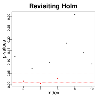
Figure 2: Example of Revisiting-Holm procedure.

If only one hypothesis is rejected per round, then RH exactly replicates the forward stepwise selection path. To relax this assumption, suppose that $p_{(1)}<\alpha/m$ and $p_{(2)}<\alpha/m$, such that both hypotheses would be rejected on the first pass. Since $H^{\emptyset,(1)}$ was rejected, $H^{\emptyset,(2)}$ could have been tested at level-$\alpha/(m-1)$. Such a test has higher power, but was ultimately unnecessary; the conservative test conducted in the first round successfully rejected $H^{\emptyset,(2)}$.

If multiple hypotheses are rejected in a round, RH is not guaranteed to have selected the most significant feature first. Since the features were not truly sorted, it is unknown which of the two hypotheses rejected in the first pass actually had a smaller p-value; both p-values were merely smaller than $\alpha/m$. Selecting features in the wrong order is not of serious concern in the orthogonal case, because the same set of features will have been selected by the end of each testing pass. In nonorthogonal settings, however, test statistics change based on the model in which they are computed, so selecting features in a different order can lead to significantly different models.

3.3 General Case: Nonorthogonal Data

In nonorthogonal data, including covariates in the incorrect order can lead to significantly different models being selected. This is due to the test statistic being model dependent and is easiest to see by example. Table 3 gives the sequential p-values of all features in the prostate cancer data in different selected models. Two algorithms are compared: RH testing the features in sorted stepwise order (1), (2),$\ldots$,(8) (RH-sort), and RH testing the features in the reverse order (8), (7),$\ldots$, (1) (RH-rev). The reverse order provides a worst-case ordering for RH. In the table, hyphens indicate the features in the model.

Table 3: Stepwise p-values after each step.

Feature (Step)	RH-0	RH-sort-1	RH-sort-2	RH-rev-1	RH-rev-2	RH-rev-3
lcavol (1)	0.0000	-	-	0.0000	0.0000	0.0000
lweight (2)	0.0000	0.0003	-	0.0000	0.0000	0.0000
svi (3)	0.0000	0.0410	0.0424	0.0000	0.0001	0.0000
lbph (4)	0.0006	0.0041	0.1506	0.0010	0.0001	-
pgg45 (5)	0.0000	0.1453	0.0758	0.0002	0.1330	0.1078
lcp (6)	0.0000	0.7300	0.9494	0.0000	-	-
age (7)	0.0027	0.7998	0.4649	0.1352	0.1331	0.7534
gleason (8)	0.0000	0.6516	0.3592	-	-	-

Forward stepwise, RH-sort, and RH-rev consider the same p-values initially (step 0), as no features have been added to the model. These p-values are computed from simple regressions between the response and the feature of interest using an independent estimate of the error variance. While all features fall below the RH threshold, lcavol has the lowest p-value. Therefore, forward stepwise and RH-sort select the same feature on step 1. The p-values in the column RH-sort-1 are the stepwise p-values given that lcavol is in the model. Again, RH-sort and forward stepwise select the same variable, lweight, at the second step. Adjusting the stepwise p-values for the model (lcavol, lweight) results in the column RH-sort-2. All of these p-values fall above the RH threshold for the third testing pass, so the procedure terminates. The correspondence between RH-sort and forward stepwise seen here is a general property: if RH tests variables in the order determined by stepwise, then RH selects variables in the same order as stepwise.

RH-rev behaves significantly differently than RH-sort and forward stepwise. The initial p-values it considers are identical, but RH-rev tests gleason first and the test is rejected. The p-values in the column RH-rev-1 condition on gleason being in the model. Proceeding in the reverse order, the test of age is not rejected, but the test of lcp is. Column RH-rev-2 updates the stepwise p-values given the model contains gleason and lcp. Using these p-values, lbph is also rejected, and the process continues. In fact, RH-rev rejects all 8 features. Given the ordering of the features, this is at least justifiable: each subsequent feature explains a significant reduction in ESS. Even after several features are in the model, lcavol provides unique information about the response. That being said, selecting all 8 features is clearly not desirable. The next section uses a different set of rejection thresholds and mimics stepwise regression precisely on these data: we identify the RH-sort model of {lcavol, lweight} regardless of the order in which features are tested.

In nonorthogonal data, one may also object to the updating done via Definition 2 because sequential p-values are relevantly different between steps. While the same explanatory feature is being tested, the null hypothesis and sequential p-value are model dependent. Furthermore, there is, in general, no guarantee that the conditioning statement in equation (2) is accurate; a feature can become more significant in the presence of other features. The next section renders this critique obsolete by introducing a new series of testing thresholds: the adjustment made in equation (2) makes a negligible change to the effecting testing level and can be ignored with a minimal reduction in power.

4 Better Threshold Approximation

To better approximate forward stepwise, initial testing passes need to search for more significant features. As forward stepwise searches for the feature which yields the maximal improvement in R², we consider a procedure which tests for an increase in R² of $r^{s}$, $r\in(0,1)$ and $s$ is the testing pass. For example, if $r=1/2$, then the first testing pass tests for features which increase R² by 1/2, while the second pass tests for those yielding an increase of 1/4. This yields a geometrically decreasing sequence of bounds. By choosing $r$, this provides a set of algorithms which are collectively referred to as Revisiting Alpha-Investing (RAI). In order to specify the stopping criterion and fully describe RAI, we need to introduce alpha-investing (FosterS08). Afterward, we provide our performance guarantee.

4.1 Revisiting Alpha-Investing

Alpha-investing rules are similar to alpha-spending rules in that they are given an initial amount of alpha-wealth to be spent on hypothesis tests. Wealth can be considered as an allotment of error probability. Bonferroni allocates this error probability equally over all hypothesis, testing each one at level $\alpha/m$. In general, the amount spent on tests can vary. If $\alpha_{i}$ is the amount of wealth spent on test $H_{i}$, FWER is controlled when

$$\sum_{i=1}^{m}\alpha_{i}\leq\alpha.$$

In clinical trials, alpha-spending is useful due to the varying importance of hypotheses. For example, many studies include both primary and secondary endpoints. As the primary endpoint is the most important hypothesis, the majority of the alpha-wealth can be spent on it, providing higher power. Alpha-spending rules can allocate the remaining wealth equally over the secondary hypotheses. FWER is controlled and the varying importance of hypotheses is acknowledged. Interested readers are referred to DmitrienkoTB10 and references therein for more on FWER control procedures.

Alpha-investing rules are similar to alpha-spending rules except that alpha-investing rules earn a return, or contribution to their alpha-wealth, of $\omega\leq\alpha$ when tests are rejected. Therefore, the alpha-wealth after testing hypothesis $H_{i}$ is rCl W_i+1 & = W_i - α_i + ωR_i An alpha-investing strategy uses the current wealth and the history of previous rejections to determine which hypothesis to test and the amount of wealth that should be spent on it.

Intuitively, alpha-investing rules spend error probability in search of false null hypotheses to reject. Each false null that is rejected allows $\alpha$ more incorrect rejections in expectation. Alpha-investing rules merely need to spend more wealth (error probability) than the probability of error they incur. In some sense, this behavior is present in all procedures which control a proportion of false rejections. For example, if it is known that the first 9 rejections were of false hypotheses, then any 10th hypothesis can be rejected while controlling the proportion of false rejections at .1.

The only assumption an alpha-investing rule requires in order to control mFDR is that each test must be conditionally level-$\alpha$ given the sequence of rejections:

$$\mathbb{E}(V_{i}|R_{1},\ldots,R_{i-1})\leq\alpha_{i}.$$

FosterS08 assume tests are independent. Theorem 1 allows alpha-investing to be used in many more scenarios. Therefore, once Theorem 1 is proven, RH and RAI control mFDR by virtue of being alpha-investing rules.

Viewing the Holm step-down procedure as an alpha-investing rule yields RH. Given initial alpha-wealth $\alpha$ and return $\omega=\alpha$, test all hypotheses at the Bonferroni level, $\alpha/m$. This exhausts all alpha-wealth, so that the procedure terminates if no rejections are made. If a rejection is made, the procedure earns a return equal to $\alpha$ and only $m-1$ hypotheses remain. The wealth is again split evenly among all remaining hypotheses, yielding the Bonferroni threshold over $m-1$ hypotheses of $\alpha/(m-1)$. If no rejections are made in a round, then the alpha-investing rule is out of wealth and the algorithm terminates.

RAI merely provides a different sequence of levels at which to test. Psuedocode for the procedures is given in Algorithm 2. Note that the implementation in R (R_2019; rai_R) makes slight modifications to this for practical performance improvements. Most importantly, it uses a conservative estimate of error variance $\hat{\sigma}$ by using the residuals from model $M$ instead of $M\cup j$. This prevents $\hat{\sigma}$ from being recomputed for every hypothesis test. While there is a concomitant loss of power, the performance improvement is significant and we still observe strong results. RAI is well defined in any model in which it is possible to test the addition of a single feature such as generalized linear models. The testing thresholds ensure that the algorithm closely mimics forward stepwise, which provides the performance guarantees of the next subsection.

Algorithm 2 Revisiting Alpha-Investing (RAI)

  Input: Feature matrix $\mathbf{X}$, response $Y$, threshold level $r$, mFDR level $\alpha$

  Output: Model corresponding to a set of features $M\subset[m]$

  Set: $M=\emptyset$, $s=1$, wealth = $\alpha$

  while $|M|\leq m$ do

     Set $\alpha_{s}=f(r^{s})$ // Alpha determined from R² threshold; See Appendix

     for $j$ in $[m]\backslash M$ do // Loop is a testing “round” or “pass”

        wealth = wealth - $\alpha_{s}$ // Pay for test

        if wealth $<$ 0 then

           Return: $M$ // Early termination

        end if

        if $X_{j}$ increases $\text{R}^{2}_{M}$ by $r^{s}$ then

           $M=M\cup j$; wealth = wealth + $\alpha$

        end if

     end for

     $s$ = $s$ + 1 // Next testing pass

  end while

  Return: $M=[m]$ // All hypotheses rejected

Approximating stepwise using these thresholds has many practical performance benefits. First, multiple passes can be made without any rejections before the algorithm exhausts its alpha-wealth and terminates. The initial tests are extremely conservative but only spend tiny amounts of wealth; however, tests rejected in these stages still earn the full return $\omega$. This ensures that wealth is not wasted too quickly when testing true null hypotheses. Furthermore, false hypotheses are not rejected using significantly more wealth than is required. An alternative construction of alpha-investing makes this latter benefit explicit and is explained in FosterS08. Taken together, this improves power in ways not addressed by the theorem in the next section. By earning more alpha-wealth, future tests can be conducted at higher power while maintaining mFDR control.

RAI performs a sequential search for sufficient model improvement as opposed to the global search for maximal improvement performed by forward stepwise. Most sequential, or online, algorithms are online in the observations, whereas RAI is online in the features. This allows features to be generated dynamically and allows extremely large data sets to be loaded into RAM one feature at a time. As such, RAI is trivially parallelizable in the MapReduce setting, similar to (Kumar+13). For example, many processors can be used, each considering a disjoint set of features. Control need only be passed to the master node when a significant feature is identified or a testing pass is completed. Parallelizing RAI will be particularly effective in extremely sparse models, such as those considered in genome-wide association studies. Online feature generation is beneficial when features are costly to generate and can be used for directed exploration of complex spaces. This is particularly useful when querying data base or searching interaction spaces as in Section 5.

Variance inflation factor regression (VIF) (LinFU11) computes stepwise t-statistics extremely quickly with little loss in accuracy. With this enhancement, RAI performs forward stepwise and model selection in $O(nm\log(n))$ time as opposed to the $O(nm^{2}q^{2})$ required for traditional forward stepwise, where $q$ is the size of the selected model. The log term is an upper bound on the number of testing passes performed by RAI. This is significantly reduced for large $n$ by recognizing when passes may be skipped, which is possible whenever a full pass is made without any rejections. The control provided by alpha-investing is maintained, because RAI must pay for all of the skipped tests. Using this computational shortcut, we find that only 7-10 passes are required to select a model using RAI.

4.2 Approximation Guarantee

This subsection bounds the performance of RAI and requires additional notation. We will often need to consider a feature $\mathbf{X}_{i}$ orthogonal to those currently in the model, $\mathbf{X}_{M}$. This will be referred to as adjusting $\mathbf{X}_{i}$ for $\mathbf{X}_{M}$ and the corresponding feature is denoted $\mathbf{X}_{i.M}=P_{M^{\perp}}\mathbf{X}_{i}$. This same notation holds for sets of variables: $\mathbf{X}_{A}$ adjusted for $\mathbf{X}_{M}$ is $\mathbf{X}_{A.M}=P_{M^{\perp}}\mathbf{X}_{A}$.

RAI is proven to perform well if the improvement in fit obtained by adding a set of features to a model is upper bounded by the sum of the improvements of adding the features individually. If a large set of features improves the model fit when considered together, this constraint requires some subsets of those features to improve the fit as well. Consider the improvement in model fit by adding $\mathbf{X}_{S}$ to the model $\mathbf{X}_{M}$:

$$\Delta_{M}(S):=\text{R${}^{2}$}(S\cup M)-\text{R${}^{2}$}(M).$$

Letting $S=A\cup B$, we bound $\Delta_{M}(S)$ as rCl Δ_M(A) + Δ_M(B) & ≥ Δ_M(S).

If $A\cup B$ improves the model fit, equation (4.2) requires that either $A$ or $B$ improve the fit. Therefore, signal that is present due to complex relationships among features cannot be completely hidden when considering subsets of these features. Equation (4.2) defines a submodular function:

Definition 3 (Submodular Function).

Let $F:2^{[m]}\rightarrow\mathbb{R}$ be a set function defined on the the power set of $[m]$. $F$ is submodular if $\forall A,B\subset[m]$ rCl F(A) + F(B) & ≥ F(A ∪B) +F(A ∩B)

This can be rewritten in the style of (4.2) as rCl F(A) - F(A∩B) + F(B) - F(A ∩B) & ≥ F(A ∪B) - F(A ∩B)
⇒Δ_A∩B(A) + Δ_A∩B(B) ≥ Δ_A∩B(A∪B), which considers the impact of $A\backslash B$ and $B\backslash A$ given $A\cap B$. Given (4.2), it is natural to approximate the maximizer of a submodular function with a greedy algorithm. We provide a proof of the performance of RAI by assuming that R² is approximately submodular.

In order for these results to hold even more generally, the definition of submodularity can be relaxed (DasK11). To do so, iterate (4.2) until the left hand side is a function of the influences of individual features and only require the inequality to hold up to a multiplicative constant $\gamma\geq 0$. Given a model $M$, consider adding the features in $A=\{a_{i},\ldots,a_{l}\}\subset[m]\backslash M$. Hence $\Delta_{M}(a_{i})$ is the marginal increase in R² by adding $a_{i}$ to model $M$. When data is normalized, $\Delta_{M}(a_{i})$ is the squared partial-correlation between the response $Y$ and $a_{i}$ given $M$: $\Delta_{M}(a_{i})=\text{Cor}(Y,a_{i.M})^{2}$. Define the vector of partial correlations as $r_{Y,A.M}=\text{Cor}(Y,A.M)$, then the sum of individual contributions to R² is $\|r_{Y,A.M}\|_{2}^{2}$. Similarly, if we define $C_{A.M}$ as the correlation matrix of $A.M$, then $\Delta_{M}(A)=r_{Y,A.M}^{\prime}C_{A.M}^{-1}r_{Y,A.M}$.

Definition 4.

(Submodularity Ratio) The submodularity ratio, $\gamma_{sr}$, of R² with respect to a model $M$ and $k\geq 1$ is rCl γ_sr(M,k) & = min_(S:S∩M = ∅, —S— ≤k) rY,S.M’rY,S.MrY,S.M’CS.M-1rY,S.M

The minimization identifies the worst case set $S$ to add to the model $M$. It captures how much R² can increase by adding $S$ to $M$ (denominator) compared to the combined benefits of adding its elements to $M$ individually (numerator). If $M$ is the size-$k$ set selected by forward stepwise, then R² is approximately submodular if $\gamma_{sr}(M,k)>\gamma$, for some constant $\gamma>0$. We will refer to data as being approximately submodular if R² is approximately submodular on the data. R² is submodular if $\gamma_{(M,2)}\geq 1$ for all $M\subset[m]$ (John+15sub). This definition is extremely similar to that of DasK11, but slightly more refined.

Our main theoretical result provides a performance guarantee for a slightly modified version of RAI. RAI has to be modified in order to account for the fact that there is, in general, no constraint on the behavior of p-values for tests of the same feature in different models. The submodularity ratio will allow us to make some claims about the improvement in R² when adding sets of features, but the control it provides on the change of individual p-values is quite poor, particularly if the model has changed significantly between two tests of the same feature. While the previous section demonstrates that we can still use the p-value in order to test a hypothesis, it does not specify any relationship between the observed p-values for testing $H^{M,j}$ and $H^{M^{\prime},j}$, when $M\neq M^{\prime}$.

The modified procedure, RAI⁺, is almost identical to RAI, in that it uses an increasing sequence of threshold values and tests features sequentially. The testing threshold, however, is not increased until all features fail to be rejected in a single model. The performance of this procedure is effectively identical to RAI. That being said, the performance guarantee requires a single model in which features can be compared. Therefore, we will refer to a testing pass of RAI⁺ as all tests using a given threshold. This single pass may cycle through all of the features multiple times. In the worst case, RAI⁺ cycles through all features in order to reject only one feature, thus not making any computational improvement over stepwise regression. This, however, is highly unlikely and is never observed in our examples. Furthermore, once all features have been tested in the same model, RAI⁺ can skip to the round in which the next feature would be rejected. Therefore in practice, RAI⁺ and RAI perform approximately the same number of computations.

We restate the essential components of Theorem 2 to make the subsequent discussion easier to follow. The model selected by RAI⁺, $M_{l}$, satisfies $\text{R${}^{2}$}(M_{l})\geq(1-e^{l/c})\text{R${}^{2}$}(M_{k}^{*})$, where $c=\left(\frac{\iota+k}{\gamma r}-\iota\right)$ and $\iota$ is the maximum number of features rejected in a testing pass. While the proof is deferred to Appendix LABEL:app:performance, a few remarks are in order.

1. This bound holds for any number of rejected features $l$. Therefore, the result in some sense mirrors the results of alpha-investing in which type-I error is controlled at any stopping time. It is more flexible, however, as $l>k$ can be considered. In this way, one can use RAI or RAI⁺ to over-estimate the support of the true model while still maintaining a performance guarantee.

2. In usual application, $l$ is actually chosen adaptively and $M_{l}$ would presumably include many of the features of $M_{k}^{*}$. Neither of these facts are leveraged in the proof; it is a worst-case guarantee assuming that $M_{l}\cap M_{k}^{*}=\emptyset$.

3. The value $\iota$ is upper bounded by $l$, but in practice is far smaller. Furthermore, it is computed while running RAI⁺. Therefore the exact value can be used in the bound after the procedure has terminated. Alternatively, $l$ could be chosen such that $\iota$ is small. This may be helpful when the last testing pass rejects a large number of features, for example.

4. The proof demonstrates an important fact that also arises in SURE (FanL08): it is important to bound the effect of adding sets of features at the same time, not the effect of adding individual features. Stronger claims could be made if we were willing to make the style of assumptions in SURE, in which they bound characteristics of each individual feature. Instead, we opt for a bound on the submodularity ratio, which is weaker but still provides a performance guarantee.

4.3 Exact Forward Stepwise

In this section, we further examine the setting $r\to 1$. This allows RAI to exactly mimic forward stepwise. Furthermore, the algorithms need not actually be run as the resulting behavior can be computed in closed form. As $r\to 1$, RAI conducts tests at level $\alpha_{s}\to 0$, $\forall s$. For concreteness, suppose that $\alpha_{s}=\delta>0$, $\forall s$. Note that repeatedly testing a hypothesis at level $\delta$ leads to an approximately linear increase in the rejection threshold by Definition 2, because $2\delta-\delta^{2}\approx 2\delta$. For sufficiently small $\delta$, this procedure selects variables in the same order as forward stepwise.

Consider the amount of wealth spent to reject a null hypothesis $H_{0}$ if its p-value is $p_{0}$. Each failed rejection implies that $p_{0}$ is in the upper $(1-\delta)$ portion of its feasible region, which is initially $[0,1]$. If $H_{0}$ is rejected after $q$ tests, a Taylor approximation provides rCl (1-δ)^q & = 1-p_0
⇒qδ ≈ -log(1-p_0). While $H_{0}$ could have been rejected by spending $p_{0}$ initially, $-\log(1-p_{0})>p_{0}$ was spent on the rejection. If $p_{0}$ is small, the amount of alpha-wealth wasted by revisiting is minor, but larger p-values waste significant wealth.

Combining the above claims, the results of RAI can be derived in closed form. Since hypotheses are rejected in the stepwise order using the sequential p-values, suppose $H_{[m]}$ is the set of hypotheses ordered by forward stepwise with corresponding p-values $p_{[m]}$. The first hypothesis is only rejected if RAI spends $\delta$ to test all hypotheses until a total of $-\log(1-p_{1})$ has been spent on each test. Similarly, the second hypothesis is only rejected if RAI continues to spend $\delta$ to test all remaining hypotheses until $-\log(1-p_{2})$ has been spent. Note that we ignore the update of equation (2) as the hypotheses are not assumed to be independent and the update is significant in this case. The resulting procedure, Stepwise-RAI (S-RAI), is given in Algorithm 3.

Algorithm 3 Stepwise Revisiting Alpha-Investing (S-RAI)

  Input: Hypotheses determined by forward stepwise, $H_{[m]}$ and corresponding sequential p-values, $p_{[m]}$.

  Set: $\hat{k}=\max\{k$ s.t. $-\sum_{i=1}^{l}(m-i+1)\log(1-p_{i})<l\alpha$, $\forall l\leq k\}$

  Reject $H_{1},\ldots,H_{\hat{k}}$

Given a full set of p-values as those in Table 2, selecting a model using hypothesis testing requires rejecting an initial contiguous set of hypotheses. If hypotheses are ordered numerically, $H_{2}$ and $H_{4}$ cannot be the only rejections. The sets $\{H_{1},H_{2}\}$ or $\{H_{1},\ldots,H_{4}\}$ are possible rejection sets that identify forward stepwise models. As p-values are not necessarily sorted by size as required by the BH procedure, controlling FDR under this constraint is nontrivial. GSell+15 transform p-values such that they are ordered and use BH on the transformed p-values. The model selection criteria they consider is ForwardStop (FS), which rejects hypotheses $H_{1},\ldots,H_{\hat{k}}$ where rCl ^k & = max_k∈{1,…,m} -1k∑_i=1^k log(1-p_i) ≤α.

Observe that the p-value transformations in equations (4.3) and (3) are identical. The conversion necessary to apply FS is equivalent to spending wealth in a wasteful way. This wastefulness is one explanation for the extremely conservative behavior of FS. Given the adjusted p-values in Table 2 are also conservative in large regions of the parameter space, it is not surprising that the combined procedure is highly conservative as demonstrated in the next section.

Under independence, S-RAI simplifies and looks very similar to FS, because the wealth spent on the unrejected hypotheses can be carried over to further rounds. Therefore, the second hypothesis would be rejected by S-RAI when an additional $-\log(1-p_{2})-\log(1-p_{1})$ has been spent. The result of this simplification is given in Algorithm 4. This provides a second way of viewing FS through a sequential lens: it performs S-RAI assuming independence but adapts to the correct subset of features. Specifically, if there were only $\hat{k}$ features instead of $m$ features, the stopping rule for FS and Algorithm 4 would be identical.

Algorithm 4 Stepwise Revisiting Alpha-Investing (S-RAI): Independent P-values

  Input: Hypotheses determined by forward stepwise, $H_{[m]}$ and corresponding sequential p-values, $p_{[m]}$.

  Set: $\hat{k}$ = $\max\{k|-\sum_{i=0}^{l-1}\log(1-p_{i})+(m-k+1)-\log(1-p_{l})<l\alpha,\forall l\leq k\}$

  Reject $H_{1},\ldots,H_{\hat{k}}$

4.4 Comparing Methods

backgroundcolor=blue!20!white,inline, bordercolor=red]need to check for other methods to potentially include

Before comparing the performance of the algorithms on data, we must discuss the interpretation of sequential tests. When features are correlated, the truth value of the null hypothesis for testing feature $j$ in model $M$, $H^{M,j}$, may depend on $M$. Hence $H^{M,j}$ may be false given the currently model M, and $\mathbf{X}_{j}$ may be correctly included at that step. Within a later active model, $M^{\prime}\supset M$, $H^{M^{\prime},j}$ may be true. Thus, a correct selection at a given step may become “incorrect” as the process proceeds, and vice-versa. This phenomenon is due to deviations from submodularity and is often called suppression (John+15sub). Our measures of false rejections are model dependent. We are not penalized if a feature which was correctly rejected is later deemed an incorrect rejection: the quality of a decision is determined at the time in which the decision was made.

While there are concerns over the “exact” description of the adjusted p-values in Table 2, one could still use them for model selection. This is particularly salient as the R package selectiveInference (selInf_R) which implements the procedure reports a statistic that does precisely that. Similarly, RH is only exact under orthogonality. We are nevertheless interested in their empirical performance when that assumption is violated. Conversely, RAI and RAI⁺ use intentionally conservative tests by not adjusting for selection as in Definition 2.

Our simulated data has $n=400$ observations, $m\in\{100,200\}$ features, of which $k\in\{20,40\}$ have a non-zero parameter value. Each feature with a non-zero parameter has a correlated counterpart with a parameter of zero. We consider correlations between each pair of features $\rho\in\{.2,.8\}$. The remaining features are orthogonal to all others in the population model. As $\mathbf{X}$ is generated randomly, the maximal correlation between such orthogonal features in a given data set is still approximately .2.

Signal strengths were chosen to be close to the RIC threshold (FosterG94). The high-signal case sets the magnitude of non-zero parameters equal to $\sqrt{4\log(m)}/\sqrt{n}$ and the low-signal case sets them to $\sqrt{2\log(m)}/\sqrt{n}$. True features in the high-signal case have t-statistics in the true model in the range $[2,7]$, while the low-signal case produces t-statistics in the true model in the range in the range $[1,5]$. As a final complication, the signs of the nonzero parameters alternate as this helps produce deviations from submodularity.

Comparisons are made between forward stepwise models selected via six procedures: forward stepwise stopped by CP, RH, RAI, RAI⁺, FS, and Stepwise Holm (equivalently Max-t or SH). Stepwise Holm merely compares the sequential p-value to the Holm threshold without any adjustments for selection. Since RH, RAI, and RAI⁺ depend on the order in which features are tested, we provided a worst case ordering: features are reordered according to the stepwise selection path, such that $\mathbf{X}_{i}$ is selected on the $i$’th step. Features are then tested from $\mathbf{X}_{m}$ to $\mathbf{X}_{1}$. This ensures that all “incorrect” features must be tested before the “correct” stepwise feature.

We report four statistics as performance measures computed over 100 repetitions of each data generating scenario: FDR, mFDR, power, and the proportion of stepwise features selected. Note that an individual false rejection is a function of our null hypothesis: if the correct feature in a group has not been included, then including the correlated counterpart is not considered a false rejection. Due to the correlation between features, such a feature legitimately improves the predictive performance of the resulting linear model. This is the same definition of false rejections used by GSellHT13.

We compute power as the proportion of features with a non-zero parameter value in the true model that are included in the final model. This allows us to consider correct selections in a classical setting in which a true model $M^{*}$ with parameters $\beta^{*}_{M^{*}}\neq 0$ exist. If an algorithm selects model $M$, then

$$\text{Power}:=\frac{|M\cap M^{*}|}{|M^{*}|}.$$

The proportion of stepwise features selected is only reported for RH, RAI, and RAI⁺. It measures the proportion of features in the selected model $M$ that are in the forward stepwise model of the same size. Given the ordering of our data matrix $\mathbf{X}$, and a selected model $M$ of size $l$, this corresponds to

$$\text{Proportion of Stepwise Features}:=\frac{|\mathbf{X}_{1:l}\cap M|}{l}.$$

Figure 3 shows the FDR and power of the six methods over the simulation settings. The x-axis is ordered such that the power of RAI is decreasing left-to-right. As such, we call this dimension the “difficulty” of the data scenario and the mapping between difficulty and simulation settings is given in Table 4. FDR is shown here for its familiarity and to demonstrate that FDR control and mFDR control are extremely similar in practice. See Figure 3 for graphs involving mFDR.

Table 4: Simulation settings and corresponding difficulty rating determined by the power of RAI. Note that difficulty essentially sorts via signal strength then correlation.

k	m	Signal	$\rho$	Difficulty	k	m	Signal	$\rho$	Difficulty
40	100	high	0.2	1	40	100	low	0.2	9
40	200	high	0.2	2	20	100	low	0.2	10
20	100	high	0.2	3	40	200	low	0.2	11
20	200	high	0.2	4	40	100	low	0.8	12
40	100	high	0.8	5	20	200	low	0.2	13
20	100	high	0.8	6	20	100	low	0.8	14
20	200	high	0.8	7	20	200	low	0.8	15
40	200	high	0.8	8	40	200	low	0.8	16

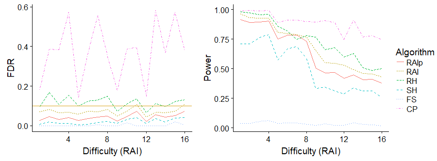
Figure 3: Performance measures. The x-axis is ordered such that the power of RAI is decreasing left-to-right. The simulation settings corresponding to this ordering are in Table 4. To demonstrate its impact, RAI uses the conditioning update of equation (2) while RAI⁺ is conservative and does not.

There are many messages conveyed by Figure 3. First, while SH is conservative, it still performs very well. This is especially telling as Taylor+14 demonstrate that the test statistic is highly conservative after multiple steps. As pointed out in Section 3.1, this is because future tests only occur if previous tests have been rejected. On this subset of cases, the test-statistics considered by SH are much less constrained. SH has significantly higher power than FS, which is so conservative as to barely reject any hypotheses in any scenario.

Second, RAI and RAI⁺ have high power while controlling FDR. Given that all methods either select a model on the stepwise path or an approximation of it, there is a necessary trade-off between power and FDR. If there is a mix of incorrect and correct features along the stepwise path, then the only way to include more correct features is to make false rejections. Therefore, one must separate the blame, so to speak, of the performance of the procedures. Part of it is the result of the testing procedure, but part is due to stepwise. The latter is suffered by all algorithms. That being said, our revisiting procedures solve the former far better than the competitor FS. Lastly, note that the FDR of CP fluctuates so rapidly because it is sensitive to the number of features $m$.

Figure 3 demonstrates the control provided in Corollary 1 and our close approximation of forward stepwise. Both Figure 3 and Figure 3 show that RH achieves high power but at the cost of losing mFDR control. As expected, it does not mimic forward stepwise well; only approximately 65-70% of the selected features are along the stepwise path of the same length. RAI and RAI⁺, on the other hand, include a high proportion of the forward stepwise features but still control false discoveries. Note that all three revisiting procedures produce models that have effectively the exact same R² as the stepwise model of the same size, merely with different covariates.

5 Searching Interaction Spaces

As an application of RAI, we demonstrate a principled method to search interaction spaces while controlling type-I errors. This has become a question of increasing interest in searching for interaction effects between genes (genesInteract11; genesInteract15). In this case, submodularity is merely a formalism of the principle of marginality (Nelder77): if an interaction between two features is included in the multiple regression, the constituent features should be as well. This reflects a belief that an interaction is only informative if the marginal terms are as well. RAI can perform a greedy search for main effects, while maintaining the flexibility to add polynomials to the model that were not in the original feature space. Therefore, we search interaction spaces in the following way: run RAI on the marginal data $\mathbf{X}$; for $i,j\in[m]$, if $\mathbf{X}_{i}$ and $\mathbf{X}_{j}$ are rejected, test their interaction by including it in the stepwise routine. We allow $i=j$ so that polynomials of a single feature are also included. This bypasses the need to explicitly enumerate the interaction space, which is computationally infeasible for large problems. Furthermore, as Table 1 shows for the concrete compressive strength data, it can be highly beneficial to only consider relevant portions of interaction spaces, as the full space is often too complex. This procedure for searching interactions was also considered in HaoZ17. We provide an efficient algorithm, an associated R package, and the following performance guarantee for the method.

As RAI⁺ is a conservative procedure, it often makes a complete pass through the data using a fixed model before termination. In this case, it is easy to bound the improvement that any single feature can provide, and this is actually computed automatically by the package. While we cannot prove that the selected model performs as well as the optimal model including all possible interactions, we are able to compare to any possible model among the set of interactions we have currently tested. Lemma LABEL:lem:Rsbnd from Appendix LABEL:app:performance yields the following corollary:

Corollary 2.

RAI⁺ selects a set of features $M$ such that adding any features $S$ that have been tested for addition to $M$ yields an improvement which is upper bounded as rCl R²(M ∪S) - R²(M) & ≤ (1-R²(M))—S—rs-1γ(M,—S—).

5.1 Simulated Data

Simulated data is used to demonstrate the ability of RAI to identify polynomials in complex spaces. Our simulated explanatory features have the following distribution:

$$\mathbf{X}_{i,j}\sim N(\tau_{j},1)\quad\text{where}\quad\tau_{j}\sim N(0,4).$$

The true mean of $Y$, $\mu_{Y}$, includes four terms which are polynomials in the first ten marginal features: rCl Y & = ϵ
μ_Y = β_1X_1X_2 + β_2X_3X_4^2 + β_3X_5X